The Finite Element Method for the Analysis of Non-Linear and ...
The Finite Element Method for the Analysis of Non-Linear and ...
The Finite Element Method for the Analysis of Non-Linear and ...

Create successful ePaper yourself
Turn your PDF publications into a flip-book with our unique Google optimized e-Paper software.
<strong>The</strong> <strong>Finite</strong> <strong>Element</strong> <strong>Method</strong> <strong>for</strong> <strong>the</strong> <strong>Analysis</strong> <strong>of</strong><br />
<strong>Non</strong>-<strong>Linear</strong> <strong>and</strong> Dynamic Systems<br />
Pr<strong>of</strong>. Dr. Eleni Chatzi<br />
Lecture 7 - 5 November, 2010<br />
Institute <strong>of</strong> Structural Engineering <strong>Method</strong> <strong>of</strong> <strong>Finite</strong> <strong>Element</strong>s II 1
Constitutive Relations<br />
Previously we examined <strong>the</strong> kinematic equations <strong>for</strong>mulation<br />
(displacement, strain displacement relations)<br />
<strong>The</strong> next step is to determine appropriate constitutive relationships<br />
<strong>of</strong> <strong>the</strong> <strong>for</strong>m:<br />
ex. linear analysis ⇒ σ = Eε<br />
σ = f(ε)<br />
When dealing with incremental analysis this is written in tensor<br />
<strong>for</strong>m <strong>for</strong> time t:<br />
t<br />
σ = t C ijrst ɛ rs<br />
Institute <strong>of</strong> Structural Engineering <strong>Method</strong> <strong>of</strong> <strong>Finite</strong> <strong>Element</strong>s II 2
Constitutive Relations<br />
It is necessary that kinematic <strong>and</strong> constitutive relations are<br />
appropriate (ex. <strong>The</strong> Second Piola-Kirchh<strong>of</strong>f stress tensor is to<br />
be used with <strong>the</strong> Green Lagrange strain tensor).<br />
Ultimately, <strong>the</strong> position <strong>of</strong> <strong>the</strong> observer frame should not affect<br />
<strong>the</strong> constitutive relations <strong>of</strong> a material (material frame<br />
indifference or objectivity <strong>of</strong> <strong>the</strong> material response).<br />
Institute <strong>of</strong> Structural Engineering <strong>Method</strong> <strong>of</strong> <strong>Finite</strong> <strong>Element</strong>s II 3
Overview <strong>of</strong> Material Descriptions<br />
We can discriminate amongst <strong>the</strong> following major classes <strong>of</strong><br />
material behavior<br />
Elastic, linear or nonlinear<br />
Hyperelastic<br />
Hypoelastic<br />
Elastoplastic<br />
Creep<br />
Viscoplastic<br />
Institute <strong>of</strong> Structural Engineering <strong>Method</strong> <strong>of</strong> <strong>Finite</strong> <strong>Element</strong>s II 4
Solution Flowchart<br />
General Solution process in incremental nonlinear FE<br />
Known Solution at t:<br />
Stresses<br />
t σ, strains t ε,<br />
Internal material parameters t κ<br />
Known Quantities at iterations i- 1 :<br />
Nodal Displacements at first Iteration:<br />
<strong>and</strong> hence<br />
<strong>Element</strong> strains<br />
t+Δt<br />
ε i−1<br />
t+Δt<br />
U i−1<br />
Calculate at t+ Δt:<br />
t+Δt<br />
Stresses σ i−1<br />
Repat till Convergence<br />
Tangent stress strain matrix C i−1<br />
Internal material parameters<br />
t+Δt<br />
κ i−1<br />
• Elastic <strong>Analysis</strong>: directly obtain<br />
t+Δt<br />
t+Δt<br />
σ i−1 , C i−1 from ε i−1<br />
• Inelastic <strong>Analysis</strong>: Integrate to get<br />
t+Δt<br />
σ i−1<br />
t t+Δti−1<br />
= σ + ∫ dσ<br />
t<br />
Calculate:<br />
Incremental Displacement Vector ΔU i:<br />
t+Δt<br />
K i−1 ΔU i =<br />
<strong>The</strong>n,<br />
t+Δt<br />
R<br />
−<br />
t+Δt<br />
F i−1<br />
t+Δt t+Δt<br />
U i = U i−1 +<br />
ΔU i<br />
Institute <strong>of</strong> Structural Engineering <strong>Method</strong> <strong>of</strong> <strong>Finite</strong> <strong>Element</strong>s II 5
Notation<br />
Main Stress - Strain pairs:<br />
Material <strong>Non</strong>linearity (small de<strong>for</strong>mations)<br />
Engineering Stress σ<br />
Engineering Strain ε<br />
TL <strong>for</strong>mulation (large de<strong>for</strong>mations)<br />
2nd Piola-Kirchh<strong>of</strong>f Stress S<br />
Green-Lagrange Strain ɛ<br />
UL <strong>for</strong>mulation (large de<strong>for</strong>mations)<br />
Cauchy Stress τ<br />
Almansi Strain ɛ A<br />
Institute <strong>of</strong> Structural Engineering <strong>Method</strong> <strong>of</strong> <strong>Finite</strong> <strong>Element</strong>s II 6
Elastic Material<br />
For an elastic material <strong>the</strong> stress is a function <strong>of</strong> strain only <strong>The</strong><br />
stress path is <strong>the</strong> same both in loading <strong>and</strong> unloading<br />
<strong>Linear</strong> Elastic<br />
<strong>The</strong> elasticity (constitutive)<br />
tensor components, C ijrs are<br />
constant<br />
<strong>Non</strong>linear Elastic<br />
<strong>The</strong> elasticity (constitutive)<br />
tensor components, C ijrs are<br />
a function <strong>of</strong> strain<br />
Example: Almost all materials under small stress<br />
σ<br />
ε<br />
Institute <strong>of</strong> Structural Engineering <strong>Method</strong> <strong>of</strong> <strong>Finite</strong> <strong>Element</strong>s II 7
Elastic Material<br />
For <strong>the</strong> case <strong>of</strong> an elastic material we already saw that <strong>the</strong> TL<br />
Formulation (used <strong>for</strong> large de<strong>for</strong>mation analysis) yields:<br />
t<br />
0S ij = t t<br />
0C ijrs 0ɛ rs<br />
<strong>The</strong> elasticity tensor <strong>for</strong> 3D stress conditions is defined as:<br />
t<br />
C ijrs = λδ ij δrs + µ(δ ir δjs + δ is δjr)<br />
where λ <strong>and</strong> µ are <strong>the</strong> Lamé constants <strong>and</strong> δ ij is <strong>the</strong> Kronecker delta,<br />
Eν<br />
λ =<br />
(ν)(1 − 2ν) , µ = E<br />
2(1 + ν)<br />
{ 0 i ≠ j<br />
δ ij =<br />
1 i = j<br />
Institute <strong>of</strong> Structural Engineering <strong>Method</strong> <strong>of</strong> <strong>Finite</strong> <strong>Element</strong>s II 8
Elastic Material<br />
Important Note<br />
“<strong>The</strong> 2nd Piola-Kirchh<strong>of</strong>f (PK2) stress <strong>and</strong> Green-Lagrange strain<br />
tensor components are invariant to rigid body motions.”<br />
For problems with small strains we can take advantage <strong>of</strong> this<br />
observation <strong>and</strong> use any constitutive relationship that has been<br />
developed <strong>for</strong> engineering stress <strong>and</strong> strain measures by just<br />
substituting with <strong>the</strong> PK2 stress <strong>and</strong> Green-Lagrange strain<br />
This observation can be extended to all problems with large<br />
de<strong>for</strong>mations but small strain conditions such as <strong>the</strong> elastic or<br />
elastoplastic buckling problem <strong>and</strong> <strong>the</strong> collapse analysis <strong>of</strong> slender<br />
structures.<br />
Institute <strong>of</strong> Structural Engineering <strong>Method</strong> <strong>of</strong> <strong>Finite</strong> <strong>Element</strong>s II 9
Elastic Material<br />
UL Formulation<br />
We now write<br />
t<br />
τ ij = t tC ∗ ijrs<br />
t tɛ A rs<br />
where <strong>the</strong> elasticity tensor components <strong>of</strong> <strong>the</strong> UL constitutive matrix<br />
C ∗ , are related to <strong>the</strong> one <strong>of</strong> <strong>the</strong> TL <strong>for</strong>mulation C, through <strong>the</strong><br />
following relationship:<br />
t<br />
tC ∗ ijrs =<br />
t<br />
ρ<br />
0<br />
ρ<br />
t<br />
0x i,m<br />
t<br />
0x j,n<br />
t<br />
0C mnpq<br />
t<br />
0x r,p<br />
t<br />
0x s,q<br />
Also <strong>the</strong> Almansi strain tensor is related to <strong>the</strong> Green-Lagrange one<br />
through<br />
t<br />
tɛ A = 0 t<br />
X T 0ɛ t 0 t<br />
X<br />
<strong>The</strong>re<strong>for</strong>e <strong>the</strong> two <strong>for</strong>mulations are equivalent <strong>and</strong> interchangeable.<br />
Institute <strong>of</strong> Structural Engineering <strong>Method</strong> <strong>of</strong> <strong>Finite</strong> <strong>Element</strong>s II 10
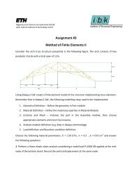
Example<br />
Consider <strong>the</strong> four node element shown below. Examine <strong>the</strong> effect <strong>of</strong> using two<br />
different stress measures <strong>and</strong> <strong>the</strong> same constitutive matrix on <strong>the</strong> Cauchy stresses.<br />
2<br />
1<br />
3 4<br />
A. TL <strong>for</strong>mulation Using <strong>the</strong> PK2 stress measure <strong>and</strong> <strong>the</strong> Green-Lagrange strain<br />
tensor we have:<br />
t<br />
0S ij = t t<br />
0C ijrs 0 ɛ rs (1)<br />
Institute <strong>of</strong> Structural Engineering <strong>Method</strong> <strong>of</strong> <strong>Finite</strong> <strong>Element</strong>s II 11
Example<br />
In order to define <strong>the</strong> required stresses <strong>and</strong> strains we need to determine <strong>the</strong> de<strong>for</strong>mation<br />
gradient t 0S, which in 2D is written as:<br />
⎡<br />
∂ t x 1 ∂ t ⎤<br />
x 1<br />
t<br />
0 X = ⎢ ∂ 0 x 1 ∂ 0 x 2<br />
⎣ ∂ t x 2 ∂ t ⎥<br />
x 2 ⎦ (2)<br />
∂ 0 x 1 ∂ 0 x 2<br />
<strong>The</strong> coordinates <strong>of</strong> a r<strong>and</strong>om point within <strong>the</strong> element are given as <strong>the</strong> weighted sum <strong>of</strong><br />
<strong>the</strong> nodal coordinates, where <strong>the</strong> weights are <strong>the</strong> shape functions. However, <strong>the</strong> shape<br />
functions are written with respect to <strong>the</strong> r, s system (isoparametric representation) as:<br />
N 1 = 1 4 (1 + r)(1 + s) N 2 = 1 (1 − r)(1 + s)<br />
4<br />
N 3 = 1 4 (1 − r)(1 − s) N 4 = 1 (3)<br />
4 (1 + r)(1 − s)<br />
From <strong>the</strong> given figure however we see that <strong>the</strong> 0 x 1 , 0 x 2 system is related to <strong>the</strong> r, s<br />
system through:<br />
0 x 1 = r + 1<br />
0 x 2 = s + 1 ⇒<br />
N 1 = 1 4 0 x 1 0 x 2 N 2 = 1 4 (2 − 0 x 1 )( 0 x 2 )<br />
(4)<br />
N 3 = 1 4 (2 − 0 x 1 )(2 − 0 x 2 ) N 4 = 1 4 0 x 1 (2 − 0 x 2 )<br />
Institute <strong>of</strong> Structural Engineering <strong>Method</strong> <strong>of</strong> <strong>Finite</strong> <strong>Element</strong>s II 12
Example<br />
<strong>The</strong>re<strong>for</strong>e, we ultimately have:<br />
∂ t x i<br />
∂ 0 x j<br />
=<br />
<strong>The</strong> nodal coordinates at time t are:<br />
4∑<br />
k=1<br />
( ) ∂Nk t x k<br />
∂ 0 i (5)<br />
x j<br />
( t x 1<br />
1<br />
, t x 1 2) = (2 + 4t, 2) ( t x 2 1, t x 2 2) = (4t, 2)<br />
( t x 3 1, t x 3 2) = (0, 0) ( t x 4 1, t x 4 2) = (2, 0)<br />
(6)<br />
By substituting (4), (5) <strong>and</strong> (6) into Eqn (2) we obtain:<br />
[ ]<br />
t 1 2t<br />
0X =<br />
0 1<br />
From Lecture 4 we know that <strong>the</strong> Green-Langrange strain tensor will <strong>the</strong>n be:<br />
t<br />
0ɛ = 1 2 (t 0X T t 0X − I) ⇒<br />
[ ]<br />
t 0 t<br />
0ɛ =<br />
t 2t 2<br />
Institute <strong>of</strong> Structural Engineering <strong>Method</strong> <strong>of</strong> <strong>Finite</strong> <strong>Element</strong>s II 13
Example<br />
Also, <strong>for</strong> plane strain strain conditions <strong>the</strong> constitutive tensor is:<br />
⎡<br />
1 ν 0<br />
C =<br />
E<br />
⎢ ν 1 0<br />
1 − ν 2 ⎣<br />
1 − ν<br />
0 0<br />
2<br />
⎤<br />
⎡<br />
E=5000,ν=0.3<br />
⎥<br />
⎢<br />
⎦ → ⎣<br />
6731 2885 0<br />
2885 6731 0<br />
0 0 1923<br />
Now, using <strong>the</strong> assumption <strong>of</strong> small strain we can use <strong>the</strong> above constitutive<br />
tensor <strong>for</strong> <strong>the</strong> relationship between <strong>the</strong> PK2 stress <strong>and</strong> <strong>the</strong> Green-Lagrange strain.<br />
Hence from Eqn (1):<br />
⎡<br />
⎢<br />
⎣<br />
S 11<br />
S 22<br />
S 12<br />
⎤<br />
⎡<br />
⎥ ⎢<br />
⎦ = ⎣<br />
5770t 2<br />
13462t 2<br />
3846t<br />
⎤<br />
⎥<br />
⎦<br />
⎤<br />
⎥<br />
⎦<br />
Institute <strong>of</strong> Structural Engineering <strong>Method</strong> <strong>of</strong> <strong>Finite</strong> <strong>Element</strong>s II 14
Example<br />
<strong>The</strong>n, <strong>the</strong> Cauchy stress at time t can be obtained from <strong>the</strong> PK2<br />
stress as (Lecture 4):<br />
t ρ t<br />
0 ρ<br />
t τ = 0X t 0S t 0X T ⇒<br />
⎡ ⎤ ⎡<br />
τ 11 21000t 2 + 54000t 4 ⎤<br />
⎢ ⎥ ⎢<br />
⎣ τ 22 ⎦ = ⎣ 13000t 2 ⎥<br />
⎦<br />
τ 12 3800t + 27000t 3<br />
Institute <strong>of</strong> Structural Engineering <strong>Method</strong> <strong>of</strong> <strong>Finite</strong> <strong>Element</strong>s II 15
Example<br />
B. Jaumann stress rate <strong>for</strong>mulation<br />
This <strong>for</strong>mulation uses <strong>the</strong> following constitutive relationship:<br />
t˜τ ij = t C ijrs t D rs (7)<br />
where <strong>the</strong> velocity strain tensor t D is computed using <strong>the</strong> velocity gradient L (see<br />
Lecture 4) :<br />
[ ]<br />
0 2<br />
L = ẊX −1 =<br />
0 0<br />
L can be decomposed to s symmetric part D = D T (<strong>the</strong> velocity strain tensor) <strong>and</strong> a<br />
skew symmetric part W = −W T (<strong>the</strong> spin tensor):<br />
L = D + W<br />
[<br />
0 1<br />
D =<br />
1 0<br />
which in this case yields<br />
] [ ]<br />
0 1<br />
, W =<br />
−1 0<br />
Now we use <strong>the</strong> same constitutive matrix C <strong>and</strong> Eqn (7) to obtain <strong>the</strong> Jaumann stress at<br />
time t:<br />
⎡ ⎤ ⎡ ⎤<br />
˜τ 11 0<br />
⎢ ⎥ ⎢ ⎥<br />
⎣ ˜τ 22 ⎦ = ⎣ 0 ⎦<br />
˜τ 12<br />
3846<br />
Institute <strong>of</strong> Structural Engineering <strong>Method</strong> <strong>of</strong> <strong>Finite</strong> <strong>Element</strong>s II 16
Example<br />
<strong>The</strong> Jaumann stress is connected to <strong>the</strong> Cauchy stress through:<br />
˜τ ij = ˙τ ij + τ ip W pj + τ jp W pi<br />
which from <strong>the</strong> above yields <strong>the</strong> follwoing <strong>for</strong>mula <strong>for</strong> <strong>the</strong> Cauchy components τ ij<br />
⎡<br />
⎢<br />
⎣<br />
˙τ 11<br />
˙τ 22<br />
˙τ 12<br />
⎤ ⎡<br />
⎥ ⎢<br />
⎦ = ⎣<br />
2τ 12<br />
⎤<br />
−2τ 12<br />
⎥<br />
⎦<br />
<strong>The</strong> above system <strong>of</strong> ordinary differential equations can be solved to finally get:<br />
⎡<br />
⎢<br />
⎣<br />
τ 11<br />
τ 22<br />
τ 12<br />
⎤ ⎡<br />
⎥ ⎢<br />
⎦ = ⎣<br />
1900(1 − cos2t)<br />
−1900(1 − cos2t)<br />
1900sin2t<br />
⎤<br />
⎥<br />
⎦<br />
<strong>The</strong> results from methods A <strong>and</strong> B are ra<strong>the</strong>r close <strong>for</strong> small values <strong>of</strong> <strong>the</strong> de<strong>for</strong>mation<br />
measure t but grow quite different as t gets larger than 0.1, indicating that <strong>the</strong> same C<br />
can no longer be used.<br />
Institute <strong>of</strong> Structural Engineering <strong>Method</strong> <strong>of</strong> <strong>Finite</strong> <strong>Element</strong>s II 17
Hyperelastic Material<br />
Hyperelastic (rubberlike) materials<br />
exhibit an incompressible response,<br />
path independence <strong>and</strong> no energy<br />
dissipation.<br />
<strong>The</strong> stress is now calculated through<br />
<strong>the</strong> strain energy functional W<br />
t<br />
0S ij = ∂W<br />
∂ t 0ɛ ij<br />
Figure: Stress-strain curves <strong>for</strong> various<br />
hyperelastic material models.<br />
Institute <strong>of</strong> Structural Engineering <strong>Method</strong> <strong>of</strong> <strong>Finite</strong> <strong>Element</strong>s II 18
Hyperelastic Material<br />
Hyperelastic Material Models<br />
Saint Venant-Kirchh<strong>of</strong>f model<br />
W (ɛ) = λ 2 [tr(ɛ)]2 + µtr(ɛ 2 )<br />
<strong>and</strong> <strong>the</strong> second Piola-Kirchh<strong>of</strong>f stress can be derived as<br />
S = λ[tr(ɛ)]I + 2µɛ<br />
λ, µ are <strong>the</strong> Lamé constants<br />
Mooney-Rivlin model<br />
W (ɛ) = C 1 (I 1 − 3) + C 2 (I 2 − 3)<br />
where C1 <strong>and</strong> C2 are empirically determined material constants <strong>and</strong><br />
I 1 = tr(C) = C 11 + C 22 + C 33<br />
where C is <strong>the</strong> Cauchy-Green de<strong>for</strong>mation tensor (see Lecture 4) <strong>and</strong><br />
I 2 = 1 2 [(I 1) 2 − tr(C) 2 ]<br />
Institute <strong>of</strong> Structural Engineering <strong>Method</strong> <strong>of</strong> <strong>Finite</strong> <strong>Element</strong>s II 19
Hypoelastic Material<br />
In this case, stress increments are calculated from strain increments<br />
dσ ij = C ijrs dɛ rs<br />
<strong>The</strong> material moduli C ijrs are defined as functions <strong>of</strong><br />
stress<br />
strain<br />
fracture criteria<br />
loading <strong>and</strong> unloading parameters<br />
maximum strains reached <strong>and</strong> so on<br />
Example Concrete models<br />
(*Hypoelasticity is not an elastic type <strong>of</strong> behavior in <strong>the</strong> sense that it<br />
does not exhibit path independence)<br />
Institute <strong>of</strong> Structural Engineering <strong>Method</strong> <strong>of</strong> <strong>Finite</strong> <strong>Element</strong>s II 20
Inelasticity<br />
Elastoplasticity, Creep <strong>and</strong> Viscoplasticity are types <strong>of</strong> Inelastic<br />
behavior<br />
Elastic behavior ⇒ stresses can be directly calculated from <strong>the</strong> strain<br />
Inelastic behavior ⇒ <strong>the</strong> stress at time t depends on <strong>the</strong> stress strain<br />
history<br />
In <strong>the</strong> incremental analysis <strong>of</strong> inelastic response we had three main scenarios<br />
Small displacements-rotations / small strains ⇒ use linear elastic<br />
solution, engineering stress <strong>and</strong> strain measures<br />
Large displacements-rotations / small strains ⇒ use TL <strong>for</strong>mulation<br />
by substituting <strong>the</strong> appropriate stress - strain measures (PK2,<br />
Green-Lagrange) in <strong>the</strong> place <strong>of</strong> <strong>the</strong> engineering stress <strong>and</strong> strain<br />
measures<br />
Large displacements-rotations / large strains ⇒ use ei<strong>the</strong>r TL or UL<br />
<strong>for</strong>mulation, more complex constitutive laws<br />
Institute <strong>of</strong> Structural Engineering <strong>Method</strong> <strong>of</strong> <strong>Finite</strong> <strong>Element</strong>s II 21
Elastoplasticity<br />
In this <strong>for</strong>mulation we encounter a linearly elastic behavior until yield<br />
<strong>and</strong> usually a gardening post yield behavior<br />
Examples Metals, soild <strong>and</strong> Rocks when subjected to high stresses<br />
Institute <strong>of</strong> Structural Engineering <strong>Method</strong> <strong>of</strong> <strong>Finite</strong> <strong>Element</strong>s II 22
Elastoplasticity<br />
<strong>The</strong> strain <strong>and</strong> stress increments are given by:<br />
dɛ rs = dɛ E rs + dɛ P rs<br />
dσ ij = C E ijrs (dɛ rs − dɛ P rs)<br />
where C E ijrs are <strong>the</strong> components <strong>of</strong> <strong>the</strong> elastic constitutive tensor <strong>and</strong> dɛ rs, dɛ E rs,<br />
dɛ P rs are <strong>the</strong> components <strong>of</strong> <strong>the</strong> total strain increment.<br />
To calculate <strong>the</strong> plastic strains we use <strong>the</strong> following three properties:<br />
Yield Function f y(σ, ɛ P )<br />
f y < 0 ⇒ Elastic behavior<br />
f y = 0 ⇒ Plastic behavior<br />
f y > 0 ⇒ Inadmissible<br />
Flow rule<br />
<strong>The</strong> yield function is used in <strong>the</strong> flow rule in order to obtain <strong>the</strong> plastic<br />
strain increments<br />
λ is a scalar to be determined<br />
dɛ P ij = λ ∂fy<br />
∂σ ij<br />
Hardening rule<br />
This specifies how <strong>the</strong> yield function is modified during plastic flow<br />
Institute <strong>of</strong> Structural Engineering <strong>Method</strong> <strong>of</strong> <strong>Finite</strong> <strong>Element</strong>s II 23
Elastoplasticity<br />
Example: Von Mises yield criterion (in 3D):<br />
f y = 0 ⇒ (σ 11 − σ 22) 2 + (σ 22 − σ 33) 2 + (σ 11 − σ 33) 2 + 6(σ 2 12 + σ 2 23 + σ 2 31) − 2σ 2 y = 0<br />
Institute <strong>of</strong> Structural Engineering <strong>Method</strong> <strong>of</strong> <strong>Finite</strong> <strong>Element</strong>s II 24
Elastoplasticity<br />
Isotropic & Kinematic hardening Rules<br />
In <strong>the</strong> case <strong>of</strong> isotropic hardening, <strong>the</strong> yield surface exp<strong>and</strong>s<br />
uni<strong>for</strong>mly.<br />
In <strong>the</strong> case <strong>of</strong> kinematic hardening, <strong>the</strong> size <strong>of</strong> <strong>the</strong> yield surface<br />
remains unchanged <strong>and</strong> <strong>the</strong> center location <strong>of</strong> <strong>the</strong> yield surface<br />
is shifted.<br />
Institute <strong>of</strong> Structural Engineering <strong>Method</strong> <strong>of</strong> <strong>Finite</strong> <strong>Element</strong>s II 25
Elastoplasticity<br />
Response <strong>for</strong> cyclic loading<br />
Isotropic hardening: <strong>the</strong> yield stress is higher as <strong>the</strong> cyclic loading progresses<br />
Kinematic hardening: <strong>the</strong> difference between unloading stress <strong>and</strong> new yield<br />
stress in <strong>the</strong> opposite direction <strong>of</strong> loading is constant <strong>and</strong> equal to 2σ y.<br />
Figure: isotropic hardening in tension<br />
Figure: kinematic hardening<br />
Institute <strong>of</strong> Structural Engineering <strong>Method</strong> <strong>of</strong> <strong>Finite</strong> <strong>Element</strong>s II 26
<strong>The</strong>rmoelastoplasticity <strong>and</strong> Creep<br />
This behavior exhibits <strong>the</strong> time effect <strong>of</strong> increasing strains under constant<br />
loads or decreasing stress under constant de<strong>for</strong>mations (relaxation)<br />
Typical examples <strong>of</strong> such behavior are metals at high temperatures<br />
<strong>The</strong> <strong>the</strong>rmal strain(ɛ = α∆T ) <strong>and</strong> <strong>the</strong> creep strain now enter <strong>the</strong><br />
<strong>for</strong>mulation <strong>of</strong> <strong>the</strong> stress strain relationships.<br />
Creep<br />
Creep is <strong>the</strong> tendency <strong>of</strong> a solid material to slowly move or de<strong>for</strong>m<br />
permanently under constant stresses. Creep tests measure <strong>the</strong> strain<br />
response due to a constant stress. <strong>The</strong> classical creep curve represents <strong>the</strong><br />
evolution <strong>of</strong> strain as a function <strong>of</strong> time in a material subjected to uniaxial<br />
stress at a constant temperature. <strong>The</strong> creep test, <strong>for</strong> instance, is per<strong>for</strong>med<br />
by applying a constant <strong>for</strong>ce/stress <strong>and</strong> analyzing <strong>the</strong> strain response <strong>of</strong> <strong>the</strong><br />
system. In general, this curve usually shows three phases or periods <strong>of</strong><br />
behavior.<br />
Institute <strong>of</strong> Structural Engineering <strong>Method</strong> <strong>of</strong> <strong>Finite</strong> <strong>Element</strong>s II 27
Creep<br />
1. A primary creep stage, also known as transient creep, is <strong>the</strong> starting stage<br />
during which hardening <strong>of</strong> <strong>the</strong> material leads to a decrease in <strong>the</strong> rate <strong>of</strong> flow<br />
which is initially very high. (0 ≤ ε ≤ ε 1).<br />
2. <strong>The</strong> secondary creep stage, also known as <strong>the</strong> steady state, is where <strong>the</strong> strain<br />
rate is constant. (ε 1 ≤ ε ≤ ε 2).<br />
3. A tertiary creep phase in which <strong>the</strong>re is an increase in <strong>the</strong> strain rate up to <strong>the</strong><br />
fracture strain. (ε 2 ≤ ε ≤ ε R).<br />
Institute <strong>of</strong> Structural Engineering <strong>Method</strong> <strong>of</strong> <strong>Finite</strong> <strong>Element</strong>s II 28
Relaxation<br />
A relaxation test is defined as <strong>the</strong> stress response due to a constant strain <strong>for</strong> a<br />
period <strong>of</strong> time. In viscoplastic materials, relaxation tests demonstrate <strong>the</strong> stress<br />
relaxation in uniaxial loading at a constant strain. <strong>The</strong> decompositon <strong>of</strong> strain<br />
rate is dε<br />
dt = dεe<br />
dt + dεvp<br />
dt<br />
<strong>The</strong> elastic part <strong>of</strong> <strong>the</strong> strain rate is given by dεe<br />
dt = dσ<br />
E−1<br />
dt<br />
For <strong>the</strong> flat region <strong>of</strong> <strong>the</strong> strain-time curve, <strong>the</strong> total strain rate is zero.<br />
Hence we have, dεvp dσ<br />
−1<br />
= −E<br />
dt<br />
dt<br />
<strong>The</strong>re<strong>for</strong>e <strong>the</strong> relaxation curve can be used to determine rate <strong>of</strong> viscoplastic strain<br />
<strong>and</strong> hence <strong>the</strong> viscosity <strong>of</strong> <strong>the</strong> dashpot in a 1D viscoplastic material model.<br />
Institute <strong>of</strong> Structural Engineering <strong>Method</strong> <strong>of</strong> <strong>Finite</strong> <strong>Element</strong>s II 29
Viscoplasticity<br />
Viscoplasticity describes <strong>the</strong> rate-dependent inelastic behavior <strong>of</strong><br />
solids. Rate-dependence in this context means that <strong>the</strong> de<strong>for</strong>mation<br />
<strong>of</strong> <strong>the</strong> material depends on <strong>the</strong> rate at which loads are applied[1].<br />
<strong>The</strong> inelastic behavior that is <strong>the</strong> subject <strong>of</strong> viscoplasticity is plastic<br />
de<strong>for</strong>mation which means that <strong>the</strong> material undergoes unrecoverable<br />
de<strong>for</strong>mations when a load level is reached. Rate-dependent plasticity<br />
is important <strong>for</strong> transient plasticity calculations.<br />
<strong>The</strong> main difference between rate-independent plastic <strong>and</strong><br />
viscoplastic material models is that <strong>the</strong> latter exhibit not only<br />
permanent de<strong>for</strong>mations after <strong>the</strong> application <strong>of</strong> loads but continue<br />
to undergo a creep flow as a function <strong>of</strong> time under <strong>the</strong> influence <strong>of</strong><br />
<strong>the</strong> applied load.<br />
Typical examples <strong>of</strong> such behavior are Polymers <strong>and</strong> Metals<br />
Institute <strong>of</strong> Structural Engineering <strong>Method</strong> <strong>of</strong> <strong>Finite</strong> <strong>Element</strong>s II 30
Viscoplasticity<br />
<strong>The</strong> elastic response <strong>of</strong> viscoplastic materials can be represented in one-dimension<br />
by Hookean spring elements. Rate-dependence can be represented by nonlinear<br />
dashpot elements.<br />
Plasticity can be accounted <strong>for</strong> by<br />
adding sliding frictional elements. In <strong>the</strong><br />
figure E is <strong>the</strong> modulus <strong>of</strong> elasticity, λ is<br />
<strong>the</strong> viscosity parameter <strong>and</strong> N is a<br />
power-law type parameter that<br />
represents non-linear dashpot<br />
σ = λ dɛ 1/N<br />
. <strong>The</strong> sliding element can<br />
dt<br />
have a yield stress (σy) that is strain<br />
rate dependent, or even constant, as<br />
shown in Figure (c).<br />
Institute <strong>of</strong> Structural Engineering <strong>Method</strong> <strong>of</strong> <strong>Finite</strong> <strong>Element</strong>s II 31
Viscoplasticity<br />
Stress-strain response <strong>of</strong> a<br />
viscoplastic material at different<br />
strain rates. <strong>The</strong> dotted lines<br />
show <strong>the</strong> response if <strong>the</strong><br />
strain-rate is held constant. <strong>The</strong><br />
blue line shows <strong>the</strong> response when<br />
<strong>the</strong> strain rate is changed<br />
suddenly.<br />
Institute <strong>of</strong> Structural Engineering <strong>Method</strong> <strong>of</strong> <strong>Finite</strong> <strong>Element</strong>s II 32
NL FE Special Considerations - <strong>The</strong> Contact Problem<br />
Difficult non linear behavior = contact between two or more<br />
bodies<br />
Contacts = From frictionless in small displacement to friction in<br />
general large strain conditions<br />
<strong>Non</strong>linearity <strong>of</strong> <strong>the</strong> analysis is not only geometric <strong>and</strong> material<br />
but also contact conditions<br />
Institute <strong>of</strong> Structural Engineering <strong>Method</strong> <strong>of</strong> <strong>Finite</strong> <strong>Element</strong>s II 33
Contact Conditions<br />
Usual term<br />
Contribution <strong>of</strong> contact<br />
<strong>for</strong>ces<br />
Consider N bodies that are in contact at<br />
time t:<br />
t S c is <strong>the</strong> complete area <strong>of</strong> contact<br />
t f c i : Components <strong>of</strong> <strong>the</strong> contact<br />
tractions t f S i : components <strong>of</strong> <strong>the</strong> known<br />
externally applied traction.<br />
<strong>The</strong>n <strong>the</strong> virtual work <strong>for</strong> <strong>the</strong> N bodies at time t is give by:<br />
Institute <strong>of</strong> Structural Engineering <strong>Method</strong> <strong>of</strong> <strong>Finite</strong> <strong>Element</strong>s II 34
Contact Conditions<br />
Usual term<br />
Cont<br />
<strong>for</strong>ce<br />
We denote <strong>the</strong> two bodies as I <strong>and</strong> J. Each body is supported such that<br />
without contact no rigid motion is possible.<br />
Institute <strong>of</strong> Structural Engineering <strong>Method</strong> <strong>of</strong> <strong>Finite</strong> <strong>Element</strong>s II 35
Definitions used in Contact <strong>Analysis</strong><br />
Let t f IJ : vector <strong>of</strong> contact surface traction on body I due to contact with<br />
body J <strong>the</strong>n t f IJ = − t f JI . Hence, <strong>the</strong> virtual work due to <strong>the</strong> contact<br />
traction can be written:<br />
∫<br />
δu I<br />
S IJ i fi IJ dS IJ +<br />
∫<br />
δu J<br />
S IJ i fi JI dS JI =<br />
∫<br />
δu IJ<br />
S IJ i fi<br />
IJ dS IJ<br />
where<br />
where<br />
δu IJ<br />
i = δu I i − δu J i<br />
We call <strong>the</strong> pair <strong>of</strong> surfaces S IJ , S IJ a contact surface pair.<br />
S IJ is named <strong>the</strong> ”contactor surface” <strong>and</strong><br />
S JI is named <strong>the</strong> ”target surface”<br />
Hence, <strong>the</strong> right h<strong>and</strong> side <strong>of</strong> <strong>the</strong> previous eqn represents <strong>the</strong> virtual work<br />
<strong>of</strong> <strong>the</strong> contact tractions over <strong>the</strong> relative virtual displacements δu I i , δuJ i<br />
Institute <strong>of</strong> Structural Engineering <strong>Method</strong> <strong>of</strong> <strong>Finite</strong> <strong>Element</strong>s II 36
Definitions used in Contact <strong>Analysis</strong><br />
Institute <strong>of</strong> Structural Engineering <strong>Method</strong> <strong>of</strong> <strong>Finite</strong> <strong>Element</strong>s II 37
Contact <strong>Analysis</strong>-Interface Conditions<br />
Normal Conditions<br />
Institute <strong>of</strong> Structural Engineering <strong>Method</strong> <strong>of</strong> <strong>Finite</strong> <strong>Element</strong>s II 38
Contact <strong>Analysis</strong>-Interface Conditions<br />
Institute <strong>of</strong> Structural Engineering <strong>Method</strong> <strong>of</strong> <strong>Finite</strong> <strong>Element</strong>s II 39
Contact <strong>Analysis</strong>-Interface Conditions<br />
Tangential Conditions<br />
Coulomb’s Law <strong>of</strong> friction States:<br />
Definitions Coulomb’s law <strong>of</strong> friction states :<br />
Institute <strong>of</strong> Structural Engineering <strong>Method</strong> <strong>of</strong> <strong>Finite</strong> <strong>Element</strong>s II 40
Contact <strong>Analysis</strong><br />
Complexities<br />
In <strong>the</strong> previous we consider pseudo-static contact conditions<br />
In dynamic analysis:<br />
Body <strong>for</strong>ces include inertial <strong>for</strong>ce effects <strong>and</strong> <strong>the</strong> kinematic interface<br />
conditions must be satisfied at all instances <strong>of</strong> time, requiring<br />
displacement, velocity <strong>and</strong> acceleration compatibility between <strong>the</strong><br />
contacting bodies.<br />
<strong>The</strong> time integrations schemes (ex. trapezoidal rule) do not<br />
automatically satisfy compatibility which <strong>the</strong>re<strong>for</strong>e has to be imposed<br />
separately on <strong>the</strong> step by step solution<br />
Various algorithms have been proposed to solve contact problems in<br />
<strong>Finite</strong> <strong>Element</strong> analysis.<br />
Institute <strong>of</strong> Structural Engineering <strong>Method</strong> <strong>of</strong> <strong>Finite</strong> <strong>Element</strong>s II 41
Contact <strong>Analysis</strong>-Solution Approach<br />
<strong>The</strong> Constraint Function <strong>Method</strong><br />
Let w be a function <strong>of</strong> λ <strong>and</strong> g such that <strong>the</strong> solutions <strong>of</strong> w(g, λ) = 0<br />
satisfy <strong>the</strong> Normal conditions<br />
Let v be a function <strong>of</strong> τ <strong>and</strong> ˙u such that <strong>the</strong> solutions v( ˙u, τ) = 0 satisfy<br />
<strong>the</strong> Tangential Conditions. <strong>The</strong>n, <strong>the</strong> contact conditions are given by:<br />
w(g, λ) = 0 v( ˙u, τ) = 0<br />
<strong>The</strong>se can now be imposed on <strong>the</strong> principle <strong>of</strong> virtual work using ei<strong>the</strong>r a<br />
penalty approach or a Lagrange Multiplier method. Variables λ <strong>and</strong> τ can<br />
be considered Lagrange multipliers, <strong>and</strong> so we consider <strong>the</strong>ir variations δλ,<br />
δτ. By multiplying by <strong>the</strong> variations <strong>and</strong> integrating in <strong>the</strong> domain we<br />
obtain <strong>the</strong> constraint equation:<br />
∫<br />
S IJ [δλ w(g, λ) + δτ u( ˙u, τ)]dS IJ = 0<br />
<strong>The</strong> governing equations <strong>of</strong> motion in this case are now both <strong>the</strong> principle<br />
<strong>of</strong> virtual work <strong>and</strong> <strong>the</strong> constraint equation<br />
Institute <strong>of</strong> Structural Engineering <strong>Method</strong> <strong>of</strong> <strong>Finite</strong> <strong>Element</strong>s II 42