The Finite Element Method for the Analysis of Non-Linear and ...
The Finite Element Method for the Analysis of Non-Linear and ...
The Finite Element Method for the Analysis of Non-Linear and ...

You also want an ePaper? Increase the reach of your titles
YUMPU automatically turns print PDFs into web optimized ePapers that Google loves.
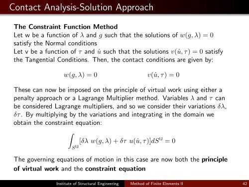
Contact <strong>Analysis</strong>-Solution Approach<br />
<strong>The</strong> Constraint Function <strong>Method</strong><br />
Let w be a function <strong>of</strong> λ <strong>and</strong> g such that <strong>the</strong> solutions <strong>of</strong> w(g, λ) = 0<br />
satisfy <strong>the</strong> Normal conditions<br />
Let v be a function <strong>of</strong> τ <strong>and</strong> ˙u such that <strong>the</strong> solutions v( ˙u, τ) = 0 satisfy<br />
<strong>the</strong> Tangential Conditions. <strong>The</strong>n, <strong>the</strong> contact conditions are given by:<br />
w(g, λ) = 0 v( ˙u, τ) = 0<br />
<strong>The</strong>se can now be imposed on <strong>the</strong> principle <strong>of</strong> virtual work using ei<strong>the</strong>r a<br />
penalty approach or a Lagrange Multiplier method. Variables λ <strong>and</strong> τ can<br />
be considered Lagrange multipliers, <strong>and</strong> so we consider <strong>the</strong>ir variations δλ,<br />
δτ. By multiplying by <strong>the</strong> variations <strong>and</strong> integrating in <strong>the</strong> domain we<br />
obtain <strong>the</strong> constraint equation:<br />
∫<br />
S IJ [δλ w(g, λ) + δτ u( ˙u, τ)]dS IJ = 0<br />
<strong>The</strong> governing equations <strong>of</strong> motion in this case are now both <strong>the</strong> principle<br />
<strong>of</strong> virtual work <strong>and</strong> <strong>the</strong> constraint equation<br />
Institute <strong>of</strong> Structural Engineering <strong>Method</strong> <strong>of</strong> <strong>Finite</strong> <strong>Element</strong>s II 42