GlowFit – a new tool for thermoluminescence glow curves doconvo

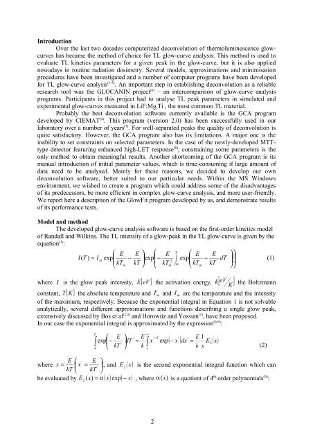
Introduction
Over the last two decades computerized deconvolution of thermoluminescence glowcurves
has became the method of choice for TL glow-curve analysis. This method is used to
evaluate TL kinetics parameters for a given peak in the glow-curve, but it is also applied
nowadays in routine radiation dosimetry. Several models, approximations and minimisation
procedures have been investigated and a number of computer programs have been developed
for TL glow-curve analysis (1-5) . An important step in establishing deconvolution as a reliable
research tool was the GLOCANIN project (6) – an intercomparison of glow-curve analysis
programs. Participants in this project had to analyse TL peak parameters in simulated and
experimental glow-curves measured in LiF:Mg,Ti , the most common TL material.
Probably the best deconvolution software currently available is the GCA program
developed by CIEMAT (4) . This program (version 2.0) has been successfully used in our
laboratory over a number of years (7) . For well-separated peaks the quality of deconvolution is
quite satisfactory. However, the GCA program also has its limitations. A major one is the
inability to set constraints on selected parameters. In the case of the newly-developed MTTtype
detector featuring enhanced high-LET response (8) , constraining some parameters is the
only method to obtain meaningful results. Another shortcoming of the GCA program is its
manual introduction of initial parameter values, which is time-consuming if large amount of
data need to be analysed. Mainly for these reasons, we decided to develop our own
deconvolution software, better suited to our particular needs. Within the MS Windows
environment, we wished to create a program which could address some of the disadvantages
of its predecessors, be more efficient in complex glow-curve analysis, and more user-friendly.
We report here a description of the GlowFit program developed by us, and demonstrate results
of its performance tests.
Model and method
The developed glow-curve analysis software is based on the first-order kinetics model
of Randall and Wilkins. The TL intensity of a glow-peak in the TL glow-curve is given by the
equation (1) :
I(
T ) = I
⎛
exp
⎜
⎝
where I is the glow peak intensity, [ eV ]
constant, [ K ]
m
E
kT
m
−
E
kT
⎞ ⎛
T
⎜
E ⎛
⎟exp
− ∫ exp
⎜
2
⎠
Tm
⎝ kTm
⎝
E
−
kT
E the activation energy, [ eV ]
k
K
the Boltzmann
T the absolute temperature and T
m and I
m are the temperature and the intensity
of the maximum, respectively. Because the exponential integral in Equation 1 is not solvable
analytically, several different approximations and functions describing a single glow peak,
extensively discussed by Bos et al (2,3) and Horowitz and Yossian (1) , have been proposed.
In our case the exponential integral is approximated by the expression (6,9) :
E
kT
m
'
⎞
⎟
⎟ ⎞
'
dT
⎠⎠
(1)
T
∫
0
' ' E 1
( − x ) dx E ( x)
∞
⎛ E ⎞ ' E ' −2
exp ⎜ − dT ≈ x exp =
'
⎟
⎝ kT ⎠ k
∫
k
x
x
2
(2)
where
E ⎛ ' E ⎞
⎜ x = ⎟ E x
kT ⎝ kT
2 is the second exponential integral function which can
⎠
E2 ( x)
= α x exp − x , where α (x)
is a quotient of 4 th order polynomials (9) :
x , and ( )
=
'
be evaluated by ( ) ( )
2