Alfredo Dubra's PhD thesis - Imperial College London
Alfredo Dubra's PhD thesis - Imperial College London
Alfredo Dubra's PhD thesis - Imperial College London

Create successful ePaper yourself
Turn your PDF publications into a flip-book with our unique Google optimized e-Paper software.
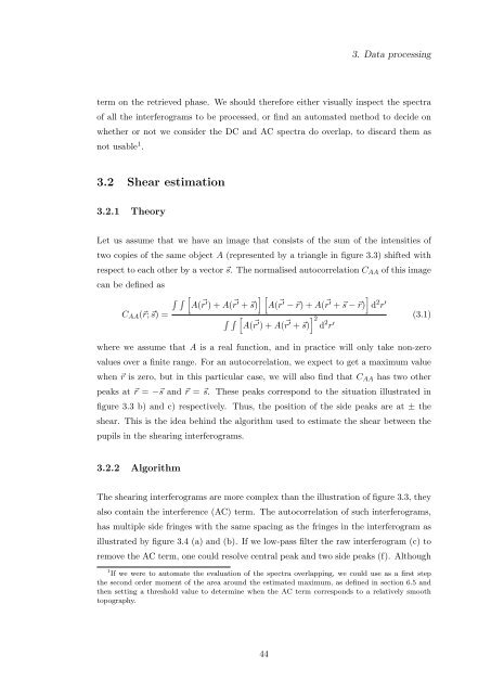
3. Data processing<br />
term on the retrieved phase. We should therefore either visually inspect the spectra<br />
of all the interferograms to be processed, or find an automated method to decide on<br />
whether or not we consider the DC and AC spectra do overlap, to discard them as<br />
not usable 1 .<br />
3.2 Shear estimation<br />
3.2.1 Theory<br />
Let us assume that we have an image that consists of the sum of the intensities of<br />
two copies of the same object A (represented by a triangle in figure 3.3) shifted with<br />
respect to each other by a vector ⃗s. The normalised autocorrelation C AA of this image<br />
can be defined as<br />
∫ ∫ [ A( r ⃗′ ) + A( ⃗ [<br />
r ′ + ⃗s)]<br />
A( r ⃗′ − ⃗r) + A( ⃗ ]<br />
r ′ + ⃗s − ⃗r) d 2 r ′<br />
C AA (⃗r; ⃗s) =<br />
∫ ∫ [ A( r ⃗′ ) + A( r ⃗ ] 2<br />
(3.1)<br />
′ + ⃗s) d 2 r ′<br />
where we assume that A is a real function, and in practice will only take non-zero<br />
values over a finite range. For an autocorrelation, we expect to get a maximum value<br />
when ⃗r is zero, but in this particular case, we will also find that C AA has two other<br />
peaks at ⃗r = −⃗s and ⃗r = ⃗s. These peaks correspond to the situation illustrated in<br />
figure 3.3 b) and c) respectively. Thus, the position of the side peaks are at ± the<br />
shear. This is the idea behind the algorithm used to estimate the shear between the<br />
pupils in the shearing interferograms.<br />
3.2.2 Algorithm<br />
The shearing interferograms are more complex than the illustration of figure 3.3, they<br />
also contain the interference (AC) term. The autocorrelation of such interferograms,<br />
has multiple side fringes with the same spacing as the fringes in the interferogram as<br />
illustrated by figure 3.4 (a) and (b). If we low-pass filter the raw interferogram (c) to<br />
remove the AC term, one could resolve central peak and two side peaks (f). Although<br />
1 If we were to automate the evaluation of the spectra overlapping, we could use as a first step<br />
the second order moment of the area around the estimated maximum, as defined in section 6.5 and<br />
then setting a threshold value to determine when the AC term corresponds to a relatively smooth<br />
topography.<br />
44