Alfredo Dubra's PhD thesis - Imperial College London

3. Data processing
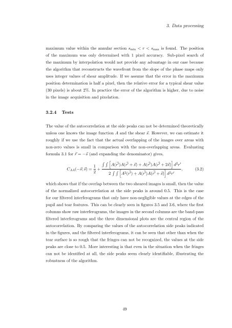
maximum value within the annular section s min < r < s max is found. The position
of the maximum was only determined with 1 pixel accuracy. Sub-pixel search of
the maximum by interpolation would not provide any advantage in our case because
the algorithm that reconstructs the wavefront from the slope of the phase maps only
uses integer values of shear amplitude. If we assume that the error in the maximum
position determination is half a pixel, then the relative error for a typical shear value
(30 pixels) is about 2%. In practice the error of the algorithm is higher, due to noise
in the image acquisition and pixelation.
3.2.4 Tests
The value of the autocorrelation at the side peaks can not be determined theoretically
unless one knows the image function A and the shear ⃗s. However, we can estimate it
roughly if we use the fact that the actual overlapping of the images over areas with
non-zero values is small in comparison with the non-overlapping areas. Evaluating
formula 3.1 for ⃗r = −⃗s (and expanding the denominator) gives,
∫ ∫ [
C AA (−⃗s; ⃗s) = 1 A( r ⃗′ )A( r ⃗′ + ⃗s) + A( r ⃗′ )A( ⃗ ]
r ′ + 2⃗s) d 2 r ′
2 + 2 ∫ ∫ [ A 2 ( r ⃗′ ) + A( r ⃗′ )A( r ⃗ ] , (3.2)
′ + ⃗s) d 2 r ′
which shows that if the overlap between the two sheared images is small, then the value
of the normalized autocorrelation at the side peaks is around 0.5. This is the case
for our filtered interferograms that only have non-negligible values at the edges of the
pupil and tear features. This can be clearly seen in figures 3.5 and 3.6, where the first
columns show raw interferograms, the images in the second columns are the band-pass
filtered interferograms and the three dimensional plots are the central region of the
autocorrelation. By comparing the values of the autocorrelation side peaks indicated
in the figures, and the filtered interferograms, it can be seen that other than when the
tear surface is so rough that the fringes can not be recognized, the values at the side
peaks are close to 0.5. More interesting is that even in the situation when the fringes
can not be identified at all, the side peaks seem clearly identifiable, illustrating the
robustness of the algorithm.
49