Stein's method, Malliavin calculus and infinite-dimensional Gaussian

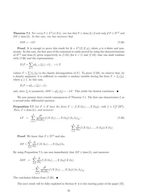
Theorem 7.1 For every F 2 L 2 ( (X)), one has that F 2 dom (L) if and only if F 2 D 1;2 and
DF 2 dom (). In this case, one has moreover that
DF = LF . (7.28)
Proof. It is enough to prove this result for H = L 2 (Z; Z; ), where is -…nite and nonatomic.
In this case, the …rst part of the statement is easily proved by using the characterizations
of D 1;2 and dom () given respectively in (7.10) (for k = 1) and (7.19), that one shall combine
with (7.26) and the representation
D z F = X q=1
qI q 1 (f q (; z)) , z 2 Z
(where F = P I q (f q ) is the chaotic decomposition of F ). To prove (7.28), we observe that, by
a density argument, it is su¢ cient to consider a random variable having the form F = I q (f q ),
where q 1. In this case,
D z F = qI q 1 (f q (; z)) ;
and, since f q is symmetric, DF = qI q (f q ) =
LF . This yields the desired conclusion.
We now present three crucial consequences of Theorem 7.1. The …rst one characterizes L as
a second-order di¤erential operator.
Proposition 7.7 Let F 2 S have the form F = f (X (h 1 ) ; :::; X (h d )), with f 2 C 1 p R d .
Then, F 2 dom (L), and moreover
LF =
dX
i;j=1
@ 2
@x i @x j
f (X (h 1 ) ; :::; X (h d )) hh i ; h j i H
(7.29)
dX
i=1
@
@x i
f (X (h 1 ) ; :::; X (h d )) X (h i ) .
Proof. We know that F 2 D 1;2 and also
DF =
dX
i=1
@
@x i
f (X (h 1 ) ; :::; X (h d )) h i .
By using Proposition 7.5, one sees immediately that DF 2 dom (), and moreover
DF =
dX
i=1
@
@x i
f (X (h 1 ) ; :::; X (h d )) X (h i )
dX
i;j=1
@ 2
@x i @x j
f (X (h 1 ) ; :::; X (h d )) hh i ; h j i H
.
The conclusion follows from (7.28).
The next result will be fully exploited in Section 9: it is the starting point of the paper [57].
35