Stein's method, Malliavin calculus and infinite-dimensional Gaussian

[21]), quadratic functionals of fractional processes (see [67]), high-frequency limit theorems on
homogeneous spaces (see [47, 48]), self-intersection local times of fractional Brownian motion
(see [33, 66]), needleets analysis on the sphere (see [1]), power variations of iterated processes (see
[55]), weighted variations of fractional processes (see [54, 63]) and of related random functions
(see [3, 16]).
10.2 Multi-dimensional CLTs
We keep the framework of the previous section. We are now interested in the normal approximation,
in the Wasserstein distance, of random vectors of multiple Wiener-Itô integrals (of possibly
di¤erent orders). In particular, our main tool is the following consequence of Theorem 9.2.
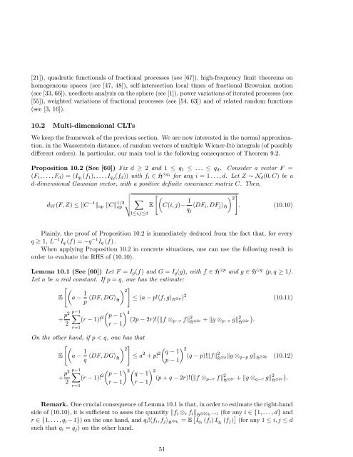
Proposition 10.2 (See [60]) Fix d 2 and 1 q 1 : : : q d . Consider a vector F =
(F 1 ; : : : ; F d ) = (I q1 (f 1 ); : : : ; I qd (f d )) with f i 2 H q i
for any i = 1 : : : ; d. Let Z N d (0; C) be a
d-dimensional Gaussian vector, with a positive de…nite covariance matrix C. Then,
v
d W (F; Z) kC 1 k op kCk 1=2 u
t X
op
1i;jd
E
"
C(i; j)
#
1
2
hDF i ; DF j i H : (10.10)
q j
Plainly, the proof of Proposition 10.2 is immediately deduced from the fact that, for every
q 1, L 1 I q (f) = q 1 I q (f) :
When applying Proposition 10.2 in concrete situations, one can use the following result in
order to evaluate the RHS of (10.10).
Lemma 10.1 (See [60]) Let F = I p (f) and G = I q (g), with f 2 H p and g 2 H q (p; q 1).
Let a be a real constant. If p = q, one has the estimate:
" #
1
2
E a
p hDF; DGi H
(a p!hf; gi H p) 2 (10.11)
+ p2
2
Xp 1 p 1 4
(r 1)! 2 (2p 2r)! kf p r fk 2 H
+ kg
r 1
2r p r gk 2
H : 2r
r=1
On the other hand, if p < q, one has that
" #
1
2 q 1 2
E a
q hDF; DGi H
a 2 + p! 2 (q p)!kfk 2 H
kg
p 1
p q p gk H 2p (10.12)
+ p2 Xp 1 p 1 2 q 1 2
(r 1)! 2 (p + q 2r)! kf p r fk 2 H
+ kg
2
r 1 r 1
2r q r gk 2
H : 2r
r=1
Remark. One crucial consequence of Lemma 10.1 is that, in order to estimate the right-hand
side of (10.10), it is su¢ cient to asses the quantity kf i r f i k H 2(q i r) (for any i 2 f1; : : : ; dg and
r 2 f1; : : : ; q i 1g) on the one hand, and q i !hf i ; f j i H q i = E I qi (f i ) I qj (f j ) (for any 1 i; j d
such that q i = q j ) on the other hand.
51