Barycentric Coordinates for Arbitrary Polygons in the Plane

More documents

Recommendations

Info

BARYCENTRIC COORDINATES FOR ARBITRARY POLYGONS 7 Let us now summarize the properties of the normalized barycentric coordinates λ i that are defined by these w i and Equation (3): 1. Affine precision. It follows from (2) and (3) that n∑ λ i (v)ϕ(v i ) = ϕ(v) i=1 for any affine function ϕ : IR 2 → IR d and v ∈ IR 2 . 2. Partition of unity. With ϕ(v) = 1 it follows immediately from the previous property that ∑ n i=1 λ i(v) = 1 for any v ∈ IR 2 . 3. Lagrange property. The functions λ i satisfy λ i (v j ) = δ i,j (see Appendix C). 4. Linearity property. The functions λ i are linear along the edges e j of Ψ (see Appendix C). 5. Linear independence. An immediate consequence of the previous property is that if ∑ n i=1 c iλ i (v) = 0 for all v ∈ IR 2 then all c i must be zero. 6. Smoothness. The functions λ i are C ∞ everywhere except at the vertices v j where they are only C 0 (see Appendix C). 7. Similarity invariance. Since the homogeneous coordinates w i depend only on areas and distances and since any uniform scale factor cancels out in the normalization (3), it follows that if ϕ : IR 2 → IR 2 is a similarity transformation 5 and ˆλ i are the normalized barycentric coordinates with respect to ̂Ψ = ϕ(Ψ), then λ i (v) = ˆλ i (ϕ(v)). 8. Locality. The homogeneous coordinate function w i depends only on the vertices v i−1 , v i , and v i+1 of Ψ. 9. Refinability. If we refine Ψ to ̂Ψ by adding the vertex ˆv = (1 − µ)v j + µv j+1 , and denote by ˆλ i and ˆλ the normalized barycentric coordinates with respect to ̂Ψ then we have λ j = ˆλ j + (1 − µ)ˆλ, λ j+1 = ˆλ j+1 + µˆλ, and λ i = ˆλ i for i ≠ j, j + 1 (see Appendix A). 10. Positivity. It follows from (11) that the functions λ i are positive inside the kernel of a star-shaped polygon and in particular inside a convex polygon. Figure 4 illustrates the typical behaviour of the functions λ i for a set of simple polygons. The main application of these generalized barycentric coordinates is the interpolation of values that are given at the vertices v i of Ψ. In other words, if a data value f i ∈ IR d is specified at each v i , then we are interested in the function F : IR 2 → IR d that is defined by n∑ n∑ F (v) = λ i (v)f i = w i (v)f i /W (v). (12) i=1 i=1 5 a translation, rotation, uniform scaling, or combination of these Technical Report IfI-05-05
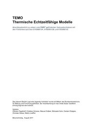
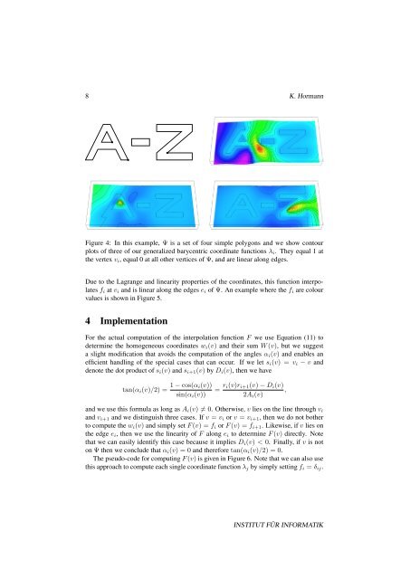
8 K. Hormann Figure 4: In this example, Ψ is a set of four simple polygons and we show contour plots of three of our generalized barycentric coordinate functions λ i . They equal 1 at the vertex v i , equal 0 at all other vertices of Ψ, and are linear along edges. Due to the Lagrange and linearity properties of the coordinates, this function interpolates f i at v i and is linear along the edges e i of Ψ. An example where the f i are colour values is shown in Figure 5. 4 Implementation For the actual computation of the interpolation function F we use Equation (11) to determine the homogeneous coordinates w i (v) and their sum W (v), but we suggest a slight modification that avoids the computation of the angles α i (v) and enables an efficient handling of the special cases that can occur. If we let s i (v) = v i − v and denote the dot product of s i (v) and s i+1 (v) by D i (v), then we have tan(α i (v)/2) = 1 − cos(α i(v)) sin(α i (v)) = r i(v)r i+1 (v) − D i (v) , 2A i (v) and we use this formula as long as A i (v) ≠ 0. Otherwise, v lies on the line through v i and v i+1 and we distinguish three cases. If v = v i or v = v i+1 , then we do not bother to compute the w i (v) and simply set F (v) = f i or F (v) = f i+1 . Likewise, if v lies on the edge e i , then we use the linearity of F along e i to determine F (v) directly. Note that we can easily identify this case because it implies D i (v) < 0. Finally, if v is not on Ψ then we conclude that α i (v) = 0 and therefore tan(α i (v)/2) = 0. The pseudo-code for computing F (v) is given in Figure 6. Note that we can also use this approach to compute each single coordinate function λ j by simply setting f i = δ ij . INSTITUT FÜR INFORMATIK
Page 1 and 2: IFI TECHNICAL REPORTS Institute of
Page 3 and 4: 2 K. Hormann In many applications i
Page 5 and 6: 4 K. Hormann (a) (b) (c) (d) (e) (f
Page 7: 6 K. Hormann Figure 3: Zero-set of
Page 11 and 12: 10 K. Hormann (a) (b) (c) (d) Figur
Page 13 and 14: 12 K. Hormann (b) (a) (c) (d) Figur
Page 15 and 16: 14 K. Hormann This is due to the la
Page 17 and 18: 16 K. Hormann (a) (b) (c) (d) Figur
Page 19 and 20: 18 K. Hormann Coxeter, H. S. M. (19
Page 21 and 22: 20 K. Hormann v j+2 v Ψ^ r j+1 α
Page 23 and 24: 22 K. Hormann twice) and also in th

Barycentric Coordinates for Arbitrary Polygons in the Plane

You also want an ePaper? Increase the reach of your titles

Delete template?

Save as template?