Propeller Design Example

prop_design_example.xls
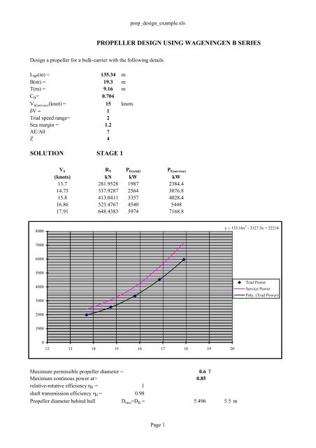
PROPELLER DESIGN USING WAGENINGEN B SERIES
Design a propeller for a bulk-carrier with the following details
L BP (m) = 135.34 m
B(m) = 19.3 m
T(m) = 9.16 m
C B = 0.704
V S(service) (knot) = 15 knots
δV = 1
Trial speed range= 2
Sea margin = 1.2
AE/A0 ?
Z 4
SOLUTION STAGE 1
V S R T P E(trial) P E(service)
(knots) kN kW kW
13.7 281.9528 1987 2384.4
14.75 337.9287 2564 3076.8
15.8 413.0411 3357 4028.4
16.86 523.4767 4540 5448
17.91 648.4383 5974 7168.8
8000
y = 135.16x 2 - 3327.5x + 22214
7000
6000
5000
4000
3000
Trial Power
Service Power
Poly. (Trial Power)
2000
1000
0
12 13 14 15 16 17 18 19 20
Maximum permissible propeller diameter =
0.6 T
Maximum continous power at= 0.85
relative-rotative efficiency η R = 1
shaft transmission efficiency η S = 0.98
Propeller diameter behind hull D max =D B = 5.496 5.5 m
Page 1

prop_design_example.xls
w = 0.304
t = 0.214
open water diameter D 0 =D B /0.95
5.79 m
A
A
(1.3
( P
+
−
0.3Z
) T
P D
E
=
2
0 0 V
)
+ K
Keller's formula
R T = 434.3604 kN at Vs=16 knots
T=R T/ (1-t)=
552.6214 kN
h=D/2+0.2 (height of shaft centre-line above base)
Atmospheric pressure, P atm = 101300 N/m 2 101300 N/m 2
Vapour pressure of water at 15 °C, P V = 1646 N/m 2 1646 N/m 2
H= T-h 6.212 m
P 0 =P atm +ρgH 163763.2 N/m 2
K= 0.2 for single screw
A E /A 0 0.482127
Wageningen B-4.55 propeller chosen
V S(trial) =
16 knots
P E(trial) = 3574.96 3575 kW
Assume η D = 0.7
P D =P E /η D 5107.143 5107 kW
V A = V S(trial) (1-w)
11.136 knots
B p =1.158(NxP 1/2 D /V 2.5 A )
δ=3.2808(NxD 0 /V A )
To find out rpm, select a range of propeller rpm, e.g. N=80~120 rpm, and calculate B p -δ
and read-off propeller efficiency, ηo at corresponding Bp-δ from the diagram:
assumed
N(rpm) Bp δ ηο
80 15.99796 136.3527 0.62
90 17.9977 153.3968 0.624
100 19.99744 170.4408 0.626
110 21.99719 187.4849 0.622
120 23.99693 204.529 0.605
0.63
0.625
0.62
0.615
0.61
0.605
y = -1E-08x 4 + 4E-06x 3 - 0.0005x 2 + 0.0282x + 0.006
0.6
80 85 90 95 100 105 110 115 120 125
Page 2

prop_design_example.xls
Optimum N
100 RPM
maximum η 0 0.626
η D =η h η R η 0 =(1-t/1-w)η R η 0 0.707
∈=η Dcalculated - η Dpreviuos
Let's assume that η D is converged
Brake power P B =(P E /η D η S )
0.007 if it is > 0.005 go back to "assume η D " and select new value
until it is 0.005
5160 kW
Installed maximum continous power =P B /0.85 6070.696844 6071 kW
Delivered power P D =P B η S
5056.89 kW
Therefore B p = 19.89882
δ = 161.9188
From B p -δ diagram at [19.89,161.92] read-off P b /D B 1
Mean face pitch=
5.50 m
Stage 2 Engine selection
calculated optimum rpm 100
Brake power(85% MCR) 5160 kW
Installed power(100% MCR) 6071 kW
Engine MAN B&W 4S60MC
N rpm Engine Power
L1 105 8160
L2 105 5200
L4 79 3920 100 5160
L3 79 6160 70 5160
79 6160 100 6071
105 8160 70 6071
NoptimumPower
100 5160 85% MCR
100 6071 100%MCR
Power (kWs)
9000
8000
7000
6000
5000
4000
3000
2000
1000
0
70 75 80 85 90 95 100 105 110
N (RPM)
Page 3

prop_design_example.xls
STAGE 3 Prediction of performance in service
Prediction of the ship speed and propeller rate of rotation in service with the engine 85% of MCR
w in service= 1.1 w in trial 0.3344
η D (assumed) 0.7
P D =P B η S
5056.89 kW
P E =P D η D
3539.823 kW
From P E (service) vs V S curve at 3539.82 kW obtain V s(service)
V S(service) =
15.3 knots
8000
y = 162.19x 2 - 3993x + 26656
7000
V PE
15.31 3539.873
6000
15.25 3482.062
5000
4000
Trial Power
Service Power
3000
Poly. (Service Power)
2000
1000
0
12 13 14 15 16 17 18 19 20
V A =V S (1-w)
10.18368 knots
B p =
0.248822 xN
δ B =
1.770605 xN
For a range of N's
N B p δ B
80 19.90575 141.6484
90 22.39396 159.3545
100 24.88218 177.0605
110 27.3704 194.7666
120 29.85862 212.4726
read-off η 0 @ intersection of Bp-δ curve with P b /D B
η 0 0.583
η D 0.688
η Dassumed -η Dcalculated
0.012 if this difference is less than 0.005 there is no need for iteration
Let's assume that η D is converged
P E(service) =P D η Dlast
3481.459 kW
Page 4

prop_design_example.xls
V S(service) =
15.25 knots
From B p -δ diagram at above intersection point read-off Bp-δ
B p 24
δ 174
V A
10.1504 knots
N=(δV A /(3.2808D))
N (service)
97.95 rpm
Therefore @ 85% MCR vessel's service speeed, V S =15.25 knots N=97.95 rpm
Page 5

prop_design_example.xls
STAGE 4. Determination of the blade surface area & B.A.R. (Cavitation control)
h=D/2+0.2 (height of shaft centre-line above base)
Atmospheric pressure, P atm = 101300 N/m 2 101300 N/m 2
Vapour pressure of water at 15 °C, P V = 1646 N/m 2 1646 N/m 2
For Trial condition
T =
9.16 m
P D =
5056.89 kW
N =
100 rpm
V A =
11.136 knots
P/D = 1
η 0 0.626
H= T-h 6.212 m
Dynamic pressure q T 224777.6 N/m 2 q T =0.5V 2 R =0.5[V 2 A +(0.7πnD) 2 ]
P 0 -Pv 162117.2 N/m 2
Cavitation number σ R =(P0-Pv)/q T 0.721234
Referring to Burrill's diagram for upper limit @ σ R , the load coefficient, τ c is read-off from fig. 4 as:
τ c 0.225
By definition
T/A p =τ c q T = 50574.96
T=P D η 0 η R /V A 552621.4 N η B =P T /P D =TV A /P D =η 0 η R
A p =T/(τ c q T ) 10.92678 m 2
Developed area from Taylor's relationship
A D =A p /(1.067-0.229xP/D) 13.03911 m 2
Blade Area Ratio
A D ≈ A E
BAR= A E /(πD 2 /4) 0.55
Selected BAR=0.55
Calculated BAR=0.55
Calculated BAR=0.55

prop_design_example.xls
Page 7