88 ON q-LAPLACE TRANSFORMS OF A GENERAL CLASS OF q ...

86 R. K. YADAV, S. D. PUROHIT AND P. NIRWAN
(ii) Again if we take N = 2, k = −2, λ = n + µ and S j,q = (q; q 2 ) j (−1) j q j(j−1) in
the theorem (2.1), we obtained the q-Laplace transform of the discrete q-Hermite
polynomial H n (x ; q) as:
{
qL s x µ+n H n (x ; q) } = (q; q) n/2
∑
n+µ
s n+µ+1
j=0
(q −n ; q) 2j (−s 2 ) j q j(j−2µ−1)
(q 2 ; q 2 ) j (q −µ ; q) 2j
· (3.2)
(iii) On setting N = 1, k = 1 and S j,q = (−1)n+j q −n(2n+1)
2 +j 2 + j 2 (p; q) n
in the
(p; q) j
main result (2.1), we obtain the q-Laplace transform of the Generalized Stieltjes-
Weigert polynomial S n (x; p; q) as:
{
qL s x λ S n (x; p, q) } [
= (−1)n q −n(2n+1)
2 (p; q) n (q; q) λ q
s λ+1 · −n , q 1+λ ;
2Φ 2
p , 0 ;
q, − q s
]
n+ 3 2
.
(3.3)
(iv) If we take N = 1, k = 1 and S j,q = (qα+n−1 ; q) j (2q) j q n(n−1)
2 −nj+ j(j−1)
2
in the
(−q; q) j
Theorem 2.1, we obtain the q-Laplace transform of the q-Bessel function of second
type y n (x; α/q 2 ) as
qL s
{
x λ y n (x; α/q 2 ) } = q n(n−1)
2 (q; q) λ
s λ+1
n ∑
j=0
(q −n ; q) j (q α+n−1 ; q) j (−2q/s) j (q λ+1 ; q) j
(q; q) j (−q; q) j
.
(3.4)
Similarly, one can deduce a number of known results due to Yadav and Purohit [15],
involving the q-Laplace images of a variety of q-polynomials as the applications of
the Theorem 2.1.
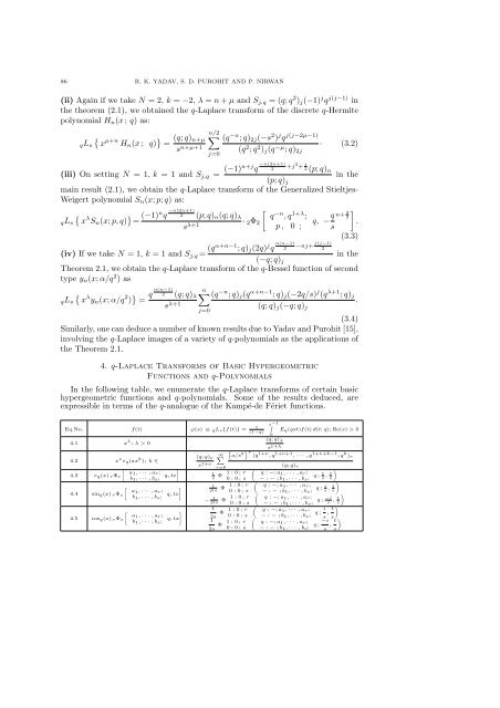
4. q-Laplace Transforms of Basic Hypergeometric
Functions and q-Polynomials
In the following table, we enumerate the q-Laplace transforms of certain basic
hypergeometric functions and q-polynomials. Some of the results deduced, are
expressible in terms of the q-analogue of the Kampé-de Fériet functions.
Eq.No. f(t) ϕ(s) ≡ q L s {f(t)} = 1
(1−q)
4.1 x λ ; λ > 0
4.2 x ν e q (ax k ); k ∈
4.3 e q (x) r Φ s
[
a1 , · · · , a r;
b 1 , · · · , b s ;
4.4 sin q(x) rΦ s
[
a1 , · · · , a r ;
b 1 , · · · , b s ;
4.5 cos q (x) r Φ s
[
a1 , · · · , a r ;
b 1 , · · · , b s;
]
q, tx
(q; q) ν
s 1+ν
∞ ∑
] 1
2is
Φ 1 : 0 ; r
q, tx
]
q, tx
s∫
−1
0
(q; q) λ
s 1+λ
E q (qst)f(t) d(t; q); Re(s) > 0
(
a/s k) r (q
1+ν , q
1+ν+1 , · · · , q
1+ν+k−1 ; q
k )r
r=0
(q; q) r
1
s
Φ 1 : 0 ; r
( )
q : −; a1 , · · · , a r;
q ;
0 : 0 ; s − : − ; b 1 , · · · , b s ;
1 s , s
t ( )
q : −; a1 , · · · , a r;
q ;
0 : 0 ; s − : − ; b 1 , · · · , b s ; s i , s
t
−
2is 1 Φ 1 : 0 ; r
( )
q : −; a1 , · · · , a r ;
q ; −i
0 : 0 ; s − : − ; b 1 , · · · , b s ; s , s
t
1
2s Φ 1 : 0 ; r
(
q : −; a1 , · · · , a r ;
q ; i 0 : 0 ; s − : − ; b 1 , · · · , b s ; s , t )
s
1
2s Φ 1 : 0 ; r
(
q : −; a1 , · · · , a r;
q ; −i
0 : 0 ; s − : − ; b 1 , · · · , b s; s , t )
s