Assessment of a Rubidium ESFADOF Edge-Filter as ... - tuprints

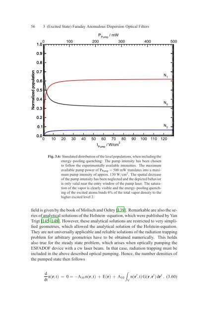
56 3 (Excited State) Faraday Anomalous Dispersion Optical Filters
P Pump
/ mW
0 1.0
100 200 300 400 500
0.9
0.8
Normalized population
0.7
0.6
0.5
0.4
0.3
0.2
0.1
N 1
N 0
N 2
0.0
0 10 20 30 40 50 60 70 80 90 100 110 120
I Pump
/ W/cm 2
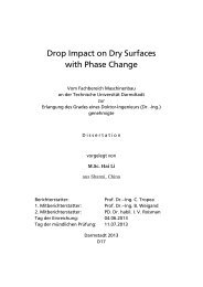
Fig. 3.6: Simulated distribution of the level populations, when including the
energy–pooling quenching: The pump intensity has been chosen
to follow the experimentally available intensities. The maximum
available pump power of P Pump = 500 mW translates into a maximum
pump intensity of approx. 130 W/cm 2 . The spatial decrease
of the pump intensity has been neglected and the depicted behavior
is only valid near the entry window of the pump laser. The saturation
of the vapor is clearly visible and the energy–pooling quenching
of the excited atoms binds 6% of the total vapor density to the
higher excited level 2.
field is given by the book of Molisch and Oehry [139]. Remarkable are also the series
of analytical solutions of the Holstein–equation, which were published by Van
Trigt [145–148]. However, these analytical solutions are restricted to very simplified
geometries, which allowed the analytical solution of the Holstein-equation.
They are not universally applicable and reliable solutions of the radiation trapping
problem for arbitrary geometries have to be obtained numerically. This holds
also true for the steady state problem, which arises when optically pumping the
ESFADOF device with a cw laser beam. In that case, radiation trapping must be
included in the above described optical pumping. Hence, the number densities of
the pumped state then follows
d
dt n(r,t) = 0 = −A 10 n(r,t) + E(r) + A 10 n(r
∫V
′ ,t)G(r,r ′ )dr ′ . (3.60)