2 DGM for elliptic problems

2 

DGM for elliptic problems 

chap:ellipt 

sec:2.0 

2.1 Model problem 

Let Ω be a bounded domain in IR d , d = 2,3, with a Lipschitz-continuous 

boundary ∂Ω. We denote by ∂Ω D and ∂Ω N parts of the boundary ∂Ω, 

Lebesques measurable with respect to (d − 1)-dimensional measure defined 

on ∂Ω, such that ∂Ω = ∂Ω D ∪ ∂Ω N and ∂Ω D ∩ ∂Ω N = ∅. 

We consider the following Poisson model problem: find a fucntion u : Ω → 

IR such that 

−∆u(x) = f(x), x ∈ Ω, (2.1) A0.1 

and 

u = u D , on ∂Ω D , (2.2) A0.2a 

n · ∇u = g N , on ∂Ω N , (2.3) A0.2b 

where f ∈ L 2 (Ω), u D ∈ L 2 (∂Ω D ) and g N ∈ L 2 (∂Ω N ). A sufficiently regular 

function satisfying ( 2.1) A0.1 – ( 2.3) A0.2b pointwise is called a classical solution. It is 

suitable to introduce the concept of a weak solution. Let us introduce the 

space 

V = {v ∈ H 1 (Ω); v| ∂ΩD = 0}. (2.4) A0.3a 

Now we multiply ( 2.1) A0.1 by a function v ∈ V , integrate over Ω and use the 

Green’s theorem. Taking into account the boundary condition ( 2.3), A0.2b we obtain 

the identity 

∫ 

∫ ∫ 

∇u · ∇v dx = f v dx + g N v dS, v ∈ V. (2.5) A0.3 

∂Ω N 

Ω 

Ω 

Let us assume the existence of u ∗ ∈ H 1 (Ω) such that u ∗ | ∂ΩD = u D . Now we 

say that a function u is a weak solution of problem ( 2.1) A0.1 - ( 2.3), A0.2b if u − u ∗ ∈ V 

and u satisfies identity ( 2.5). 

A0.3

10 2 Elliptic problems 

sec:2.1 

sec:2.1.1 

conftri 

2.2 Spaces of discontinuous functions 

2.2.1 Partition of the domain 

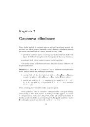
Let T h (h > 0) be a partition of the closure Ω of the domain Ω into a finite 

number of closed d-dimensional simplexes K with mutually disjoint interiors 

such that 

Ω = ⋃ 

K∈T h 

K. (2.6) A1.1 

We call T h a triangulation of Ω and do not require the standard conforming 

properties from the finite element method, introduced e.g. in [Cia79], Ciarlet [BS94], 

BrScott 

Johnson 

[Joh88], [Sch00] Schwab or [Žen90]. Zenisek In two-dimensional problems (d = 2) we choose 

K ∈ T h as triangles and in three-dimensional problems (d = 3) the elements 

K ∈ T h are tetrehedra. As we see, we admit that in the finite element mesh 

the 

fig:faces 

so-called hanging nodes (and in 3D also hanging edges) appear (see Figure 

2.1). 

Remark 2.1. Let us remind that the triangulation T h is conforming, if it has 

the following property: if K,K ′ ∈ T h , then K ∩K ′ = ∅ or K ∩K ′ is a common 

vertex or K ∩ K ′ is a common edge (or K ∩ K ′ is a common face in the case 

d = 3) of K and K ′ . 

In general, the discontinuous Galerkin method can handle with more general 

elements as quadrilaterals and convex or even nonconvex star-shaped 

polygons in 2D and hexahedra, pyramids and convex or nonconvex star-shaped 

polyhedra in 3D. As an example, we can consider the so-called dual finite volumes 

constructed over triangular (d = 2) or tetrahedral (d = 3) meshes (cf., 

e.g. [FFLMW99]). FFLW96 A use of such elements will be discussed in Section ??. 

sec:grids 

In our further considerations we shall use the following notation. By ∂K 

we denote the boundary of an element K ∈ T h and set h K = diam(K) = 

diameter of K, h = max K∈Th h K . By ρ K we denote the radius of the largest 

d-dimensional ball inscribed into K and by |K| we denote the d-dimensional 

Lebesgue measure of K. 

Let K,K ′ ∈ T h . We say that K and K ′ are neighbours, if the set ∂K ∩∂K ′ 

has positive (d − 1)-dimensional measure. We say that Γ ⊂ K is a face of K, 

if it is a maximal connected open subset either of ∂K ∩ ∂K ′ , where K ′ is a 

neighbour of K, or of ∂K ∩ ∂Ω. By F h we denote the system of all faces of 

all elements K ∈ T h . Further, we define the set of all innner faces by 

the set of all “Dirichlet” boundary faces by 

and the set of all “Neumann” boundary faces by 

F I h = {Γ ∈ F h ; Γ ⊂ Ω}, (2.7) A1.6 

F D h = {Γ ∈ F h ; Γ ⊂ ∂Ω D } (2.8) A1.7

2.2 Spaces of discontinuous functions 11 

⃗n Γ8 

Γ 5 

Γ 6 

⃗n Γ6 

Γ 8 

⃗n Γ1 

⃗n Γ2 

K 1 

K 2 

K 3 

⃗n Γ5 

K 5 

Γ 1 

Γ 2 

⃗n Γ7 

Γ 7 

Γ 4 

Γ 3 

⃗n Γ4 

⃗n Γ3 

K 4 

Fig. 2.1. Example of elements K l , l = 1, . . . , 5, and faces Γ l , l = 1, . . . , 8, with the 

corresponding normals n Γl 

fig:faces 

F N h = {Γ ∈ F h , Γ ⊂ ∂Ω N } . (2.9) A1.8 

Obviously, F h = Fh I ∪ FD h ∪ FN h 

. For a shorter notation we put 

F ID 

h = F I h ∪ F D h , F DN 

h = F D h ∪ F N h . (2.10) A1.9 

For each Γ ∈ F h we define a unit normal vector n Γ . We assume that for 

Γ ∈ Fh 

DN the normal n Γ has the same orientation as the outer normal to ∂Ω. 

For 

fig:faces 

each face Γ ∈ Fh I the orientation of n Γ is arbitrary but fixed. See Figure 

2.1. Finally, by d(Γ) we denote the diameter of Γ ∈ F h . 

sec:2.1.2 

2.2.2 Broken Sobolev spaces 

Over a triangulation T h we define the so-called broken Sobolev space 

H k (Ω, T h ) = {v;v| K ∈ H k (K) ∀K ∈ T h } (2.11) A1.12 

with the norm 

and the seminorm 

( ∑ 

‖v‖ H k (Ω,T h ) = 

|v| H k (Ω,T h ) = 

K∈T h 

‖v‖ 2 H k (K) 

) 1/2 

(2.12) A1.13 

( ) 1/2 ∑ 

. (2.13) A1.14 

K∈T h 

|v| 2 H k (K)


Γ 

⃗n Γ 

K (L) 

Γ 

K (R) 

Γ 

Fig. 2.2. Interior face Γ, elements K (L) 

Γ 

and K (R) 

Γ 

and the orientation of n Γ fig:normals 

For each Γ ∈ Fh I 

such that Γ ⊂ ∂K (L) 

Γ 

normal to the element ∂K (L) 

Γ 

Figure fig:normals 

2.2. We call elements K (L) 

Γ 

introduce the following notation: 

there exist two neighbouring elements K(L) 

Γ 

,K(R) Γ 

∈ T h 

∩ ∂K (R) 

Γ 

. We use a convention that n Γ is the outer 

v| (L) 

Γ 

v| (R) 

Γ 

and the inner normal to the element ∂K (R) 

Γ 

, see 

neighbours. For v ∈ H 1 (Ω, T h ), we 

, K(R) Γ 

= the trace of v| K 

(L) 

Γ 

= the trace of v| (R) K Γ 

) 

〈v〉 Γ 

= 1 2 

[v] Γ 

= v| (L) 

Γ 

( 

v| (L) 

Γ 

+ v|(R) Γ 

− v|(R) Γ . 

, 

on Γ, (2.14) A1.15 

on Γ, 

The value [v] Γ depends on the orientation of n Γ , but the value [v] Γ n Γ is 

independent of this orientation. 

For Γ ∈ Fh 

DN there exists element K (L) 

Γ 

∈ T h such that Γ ⊂ K (L) 

Γ 

∩ ∂Ω. 

Then for v ∈ H 1 (Ω, T h ), we introduce the following notation: 

v| (L) 

Γ 

= the trace of v| K 

(L) 

Γ 

〈v〉 Γ 

= [v] Γ 

= v| (L) 

Γ . 

on Γ, (2.15) A1.17 

For Γ ∈ Fh 

DN by v| (R) 

Γ 

we formally denote the exterior trace of v on Γ given 

either by a boundary condition or by an extrapolation from the interior of Ω. 

In case that [·] Γ , 〈 · 〉 Γ 

and n Γ appear in the integrals ∫ Γ ... dS, Γ ∈ F h, 

we omit the subscript Γ and write simply [·], 〈 · 〉 and n, respectively. 

sec:2.1.3 

2.2.3 Spaces of discontinuous piecewise polynomial functions 

As we already mentioned in Introduction, DGM is based on the use of discontinuous 

piecewise polynomial approximations.


Let T h be a triangulation of Ω introduced in Section sec:2.1.1 2.2.1 and let p ≥ 

0 be an integer. We define the space of discontinuous piecewise polynomial 

functions 

S hp = {v;v| K ∈ P p (K) ∀K ∈ T h }, (2.16) A1.23 

where P p (K) denotes the space of all polynomials on K of degree ≤ p. We 

call the number p the degree of polynomial approximation. 

sec:2.1.4 

2.2.4 Some auxiliary results 

Assumptions on the mesh 

Let us consider a system {T h } h∈(0,h0), h 0 > 0, of partitions of the domain Ω 

(T h = {K} K∈Th ). In our further considerations we shall meet the following 

assumptions. 

(A1) The system {T h } h∈(0,h0) is shape regular: there exists a positive constant 

C R such that 

h K 

ρ K 

≤ C R ∀K ∈ T h , ∀h ∈ (0,h 0 ). (2.17) A1.33 

(A2) The system {T h } h∈(0,h0) is locally quasi-uniform: there exists a constant 

C H > 0 such that 

h K ≤ C H h K ′ ∀K,K ′ ∈ T h , K,K ′ are neighbours, ∀h ∈ (0,h 0 ). (2.18) A1.35 

rem:MA 

Remark 2.2. Sometimes the quasi-uniformity of the mesh is required, i.e. there 

exists a constant ˜C > 0 such that h ≤ ˜Ch K ∀K ∈ T h . The condition ( 2.18) 

A1.35 

is weaker condition than quasi-uniformity since it only limits the ratio of 

diameters of neighbouring elements. 

Let us introduce important tools for the theoretical analysis of the DG 

method. 

lem:MTI 

Lemma 2.3. (Multiplicative trace inequality) Let assumption (A1) be 

satisfied. Then there exists a constant C M > 0 independent of v, h and K 

such that 

( 

) 

‖v‖ 2 L 2 (∂K) ≤ C M ‖v‖ L2 (K) |v| H1 (K) + h −1 

K ‖v‖2 L 2 (K) , (2.19) eq:MTI 

K ∈ T h , v ∈ H 1 (K), h ∈ (0,h 0 ). 

Proof. Let K ∈ T h be arbitrary but fixed. We denote by x K the centre of the 

largest d−dimensional ball inscribed into the simplex K. (Of course, ρ K is the 

radius of this ball.) Without the loss of generality we suppose that x K is the 

origin of the coordinate system. We start from the following relation 

∫ 

∫ 

v 2 x · ndS = ∇ · (v 2 x)dx, v ∈ H 1 (K). (2.20) A1.51 

∂K 

K


x K 

α 

x 

K 

ρ K 

Γ 

n Γ 

Fig. 2.3. Simplex K with its face Γ 

fig:dist 

Let n Γ be the unit outer normal to K on a side Γ of K. Then 

see Figure 2.3. 

fig:dist 

From ( 2.21) A1.52 we have 

∫ 

x · n Γ = |x||n Γ |cos α = |x|cos α = ρ K x ∈ Γ, (2.21) A1.52 

∂K 

= ρ K 

∑ 

v 2 x · n dS = ∑ 

Γ ⊂∂K 

∫ 

Γ 

Γ ⊂∂K 

∫ 

Γ 

v 2 dS = ρ K ‖v‖ 2 L 2 (∂K) . 

v 2 x · n Γ dS (2.22) A1.54 

Moreover, 

∫ 

∫ 

∇ · (v 2 ( 

x)dx = v 2 ∇ · x + x · ∇v 2) dx (2.23) A1.55 

K 

K 

∫ ∫ 

∫ 

= d v 2 dx + 2 vx · ∇v dx ≤ d‖v‖ 2 L 2 (K) + 2 |vx · ∇v|dx. 

K 

K 

With the aid of the Cauchy inequality, the second term of ( 2.23) A1.55 is estimated 

as 

∫ 

∫ 

2 |vx · ∇v|dx ≤ 2 sup |x| |v||∇v|dx ≤ 2h K ‖v‖ L 2 (K)|v| H 1 (K). (2.24) A1.56 

K 

x∈K K 

Then ( 2.17), A1.33 ( 2.20), A1.51 ( 2.22), A1.54 ( 2.23) A1.55 and ( 2.24) A1.56 give 

K

lem:II 

lem:III 

def:Pi_h 


‖v‖ 2 L 2 (∂K) ≤ 1 [ 

] 

2h K ‖v‖ L 

ρ 2 (K)|v| H 1 (K) + d‖v‖ 2 L 2 (K) (2.25) A1.57 

K 

[ 

≤ C R 2‖v‖ L2 (K)|v| H1 (K) + d ] 

‖v‖ 2 L 

h 2 (K) , 

K 

which proves ( eq:MTI 2.19) with C M = C R max{2,d}. ⊓⊔ 

Lemma 2.4. (Inverse inequality) Let (A1) be satisfied. Then there exists 

a constant C I > 0 independent of v, h and K such that 

|v| H1 (K) ≤ C I h −1 

K ‖v‖ L 2 (K), ∀v ∈ P p (K), ∀K ∈ T h , forallh ∈ (0,h 0 ). 

(2.26) eq:InvI 

Proof. Let ˆK be a reference triangle and F K : ˆK → K, K ∈ Th be an 

affine mapping such that F K ( ˆK) = K. By [Cia79], Ciarlet Theorem 3.1.2 for any v ∈ 

H m (K), where m ≥ 0 is an integer,the function ˆv(ˆx) = v(F K (ˆx)) ∈ H m ( ˆK) 

and 

|v| Hm (K) ≤ c c h d 2 −m 

K |ˆv| H m ( ˆK) 

, (2.27) eq:ci1 

|ˆv| Hm ( ˆK) ≤ c ch m− d 2 

K |v| H m (K), (2.28) eq:ci2 

where c c > 0 depends on C R but not on K and v. From [Sch98], Schwab-book Theorem 

4.76 we have 

|ˆv| H 1 ( ˆK) ≤ c sp 2 ‖ˆv‖ L 2 ( ˆK) , ˆv ∈ P p( ˆK), (2.29) eq:sch 

where c s > 0 depends on d but not on ˆv and p. A simple combination of ( 2.27) 

eq:ci1 

– ( 2.29) eq:sch proves ( 2.26) eq:InvI with C I = c s c 2 c p 2 . ⊓⊔ 

Lemma 2.5. (Approximation properties) Let assumption (A1) be valid. 

Then there exist a mapping π K,p : H 1 (K) → P p (K) and a constant C A > 0 

such that 

|π K,p v − v| H q (K) ≤ C A h µ−q 

K |v| H µ (K) (2.30) eq:ap 

∀v ∈ H s (K) ∀K ∈ T h ∀h ∈ (0,h 0 ), 

where µ = min(p + 1,s), 0 ≤ q ≤ s and p,s are integers. 

Proof. We define π K,p as the L 2 (K) projection on P p (K), i.e, for ϕ ∈ L 2 (K), 

∫ 

∫ 

π K,p ϕ ∈ P p (K), (π K,p ϕ)v dx = ϕv dx ∀v ∈ P p (K). (2.31) Ltwoproj 

K 

The approximation properties ( 2.30) eq:ap follow immediately from [Cia79, Ciarlet Theorem 

3.1.4]. 

⊓⊔ 

Definition 2.6. Let T h be a triangulation and p ≥ 0. We define the mapping 

Π hp : H 1 (Ω, T h ) → S hp by 

K 

(Π hp u) | K = π K,p (u| K ) ∀K ∈ T h , (2.32) eq:Pi_h 

where π K,p : H 1 (K) → P p (K) is the mapping introduced in Lemma 2.5. 

lem:III

lem:AP 


By ( 2.31), Ltwoproj π K,p is the operator of L 2 (K)-projection. This implies that Π hp 

is the L 2 (Ω)-projection on S hp : if ϕ ∈ L 2 (Ω), then 

∫ 

∫ 

Π hp ϕ ∈ S hp , (Π hp ϕ)v dx = ϕv dx ∀v ∈ S hp . (2.33) LtwoprOm 

Lemma 2.7. Let assumption (A1) be valid. Then 

Ω 

Ω 

|Π hp v − v| Hq (Ω,T h ) ≤ C Ah µ−q |v| Hµ (Ω,T h ), v ∈ H s (Ω, T h ), (2.34) eq:AP 

where µ = min(p + 1,s), 0 ≤ q ≤ s and C A is the constant from ( 2.30). 

eq:ap 

Proof. Using ( 2.32), eq:Pi_h definition of a seminorm in a broken Sobolev space and 

the approximation properties ( 2.30), eq:ap we obtain ( 2.34). eq:AP 

⊓⊔ 

sec:2.2 

2.3 DGM based on a primal formulation 

In this section we shall describe and analyze the DGM for the solution of 

problem ( 2.1) A0.1 – ( 2.3) A0.2b based on a primal formulation. The approximate solution 

will be sought in the space S hp ⊂ H 1 (Ω, T ). However, the weak formulation 

( 2.5) A0.3 given in Section 2.1 sec:2.0 is not suitable for the derivation of the DGM, because 

( 2.5) A0.3 does not make sense for u ∈ H 1 (Ω, T ) ⊄ H 1 (Ω). Therefore, we shall 

introduce a “weak form of ( 2.1) A0.1 – ( 2.3) A0.2b in the sence of broken Sobolev spaces”. 

Let as assume that u is a sufficiently regular solution of ( 2.1) A0.1 – ( 2.3). A0.2b We 

shall consider the so-called strong solution, i.e. a solution u ∈ H 2 (Ω). We 

proceed in the following way: We multiply ( 2.1) A0.1 by a function v ∈ H 2 (Ω, T h ) 

integrate over K ∈ T and use Green’s theorem. Summing over all K ∈ T h , we 

obtain the identity 

∑ 

∇u · ∇v dx − ∑ 

∫ 

(n K · ∇u)v dS = f v dx, (2.35) A2.4 

K∈T h 

∫K 

K∈T h 

∫∂K 

where n K denotes the unit outer normal to ∂K. The surface integrals over 

∂K make sense due to the regularity of u. We split them according to the 

type of faces Γ that form the boundary of the element K ∈ T h : 

∑ 

K∈T h 

∫∂K 

= ∑ 

Γ ∈F D h 

+ ∑ 

∫ 

Γ ∈F I h 

Γ 

∫ 

(n K · ∇u)v dS (2.36) A2.5 

(n Γ · ∇u)v dS + ∑ 

Γ 

( 

n Γ · 

Γ ∈F N h 

(∇u| (L) 

Γ 

)v|(L) Γ 

∫ 

Γ 

Ω 

(n Γ · ∇u)v dS 

− (∇u|(R) Γ 

)v|(R) Γ 

) 

dS. 

(There is a sign “−” in the last integral, since n Γ is the unit outer normal to 

but the unit inner normal to ∂K (R) sec:2.1.1 

Γ 

, see Section 2.2.1 or Figure 2.2. 

fig:normals 

∂K (L) 

Γ

Due to the assumption that u ∈ H 2 (Ω), 

[u] Γ = 0 = [∇u] Γ , 

2.3 DGM based on a primal formulation 17 

∇u| (L) 

Γ 

= ∇u| (R) 

Γ 

= 〈∇〉 Γ . (2.37) jumpsonGamma 

Thus, the integrand of the last integral in ( A2.5 2.36) can by written in the form 

n Γ · (∇u)| (L) 

Γ 

v|(L) Γ 

Hence, due to ( A0.2b 2.3), ( A1.17 2.15) and ( A2.4 2.35) – ( A2.6 

∫ 

= 

∑ 

K∈T h 

∫K 

Ω 

− n Γ · (∇u)| (R) 

Γ 

v|(R) Γ 

= n Γ · 〈∇u)〉 Γ 

[v] Γ . (2.38) A2.6 

∇u · ∇v dx − 

f v dx + ∑ 

Γ ∈F N h 

∫ 

Γ 

2.38), we have 

∑ ∫ 

n · 〈∇u〉 [v]dS (2.39) A2.9 

Γ ∈F ID 

h 

Γ 

g N v dS, v ∈ H 2 (Ω, T h ). 

Moreover, for u,v ∈ H 1 (Ω, T h ) we define the interior penalty bilinear form 

Jh σ (u,v) = ∑ ∫ 

σ[u][v]dS (2.40) A2.17 

and the boundary penalty linear form 

Γ ∈F ID 

h 

J σ D(v) = ∑ 

Γ ∈F D h 

∫ 

Γ 

Γ 

σu D v dS, (2.41) A2.18 

where σ > 0 is a penalty weight. Its choice will be discussed in Section 2.4. 

sec:2.4 

If u ∈ H 1 (Ω) ∩H 2 (Ω, T h ) and u satisfies the Dirichlet boundary condition 

( 2.2), A0.2a then 

∑ 

∫ 

n · 〈∇v〉 [u]dS = ∑ ∫ 

n · ∇v u D dS ∀v ∈ H 2 (Ω, T h ) (2.42) A2.E1 

and 

Γ ∈F ID 

h 

Γ 

Γ ∈F D h 

Γ 

J σ h(u,v) = J σ D(v) ∀v ∈ H 2 (Ω, T h ), (2.43) A2.E2 

since [u] Γ = 0 for Γ ∈ Fh I and [u] Γ = u| Γ = u D for Γ ∈ Fh D. 

Now, we introduce several variants of the discontinuous Galerkin weak 

formulation in such a way that we sum ( 2.39) A2.9 with −1, 0 or 1-multiple of 

( 2.42) A2.E1 and possibly add equality ( 2.43).This A2.E2 leads us to the following notation. 

For u,v ∈ H 2 (Ω, T h ) we set 

a s h(u,v) = ∑ 

K∈T h 

∫K 

− 

∑ 

Γ ∈F ID 

h 

∇u · ∇v dx (2.44) ah_S 

∫ 

Γ 

(n · 〈∇u〉 [v] + n · 〈∇u〉 [v]) dS,


a n h(u,v) = ∑ 

K∈T h 

∫K 

− 

a i h(u,v) = ∑ 

∑ 

Γ ∈F ID 

h 

K∈T h 

∫K 

∇u · ∇v dx (2.45) ah_N 

∫ 

Γ 

(n · 〈∇u〉 [v] − n · 〈∇u〉 [v]) dS, 

∇u · ∇v dx − 

∑ 

Γ ∈F ID 

h 

∫ 

Γ 

n · 〈∇u〉 [v]dS (2.46) ah_I 

and the linear forms 

∫ 

Fh(v) s = f v dx + ∑ 

∫ 

Fh n (v) = 

∫ 

Fh(v) i = 

Ω 

Ω 

Γ ∈F N h 

f v dx + ∑ 

Γ ∈F N h 

f v dx + ∑ 

Ω 

Γ ∈F N h 

∫ 

g N v dS + ∑ ∫ 

n · ∇v u D dS, (2.47) Fh_S 

∫ 

∫ 

Γ 

Γ 

Γ 

Γ ∈F D h 

g N v dS − ∑ 

∫ 

Γ 

Γ ∈F D Γ 

h 

n · ∇v u D dS, (2.48) Fh_N 

g N v dS. (2.49) Fh_I 

Moreover, for u,v ∈ H 2 (Ω, T h ) let us define the bilinear forms 

and the linear forms 

B s h(u,v) = a s h(u,v), (2.50) A2.20a 

Bh(u,v) n = a n h(u,v), (2.51) A2.20b 

B s,σ 

h (u,v) = as h(u,v) + Jh σ (u,v), (2.52) A2.20c 

B n,σ 

h (u,v) = an h(u,v) + Jh σ (u,v), (2.53) A2.20d 

B i,σ 

h (u,v) = ai h(u,v) + Jh σ (u,v) (2.54) A2.20e 

def:2.1 

l s h(v) = F s h(v), (2.55) A2.21a 

l n h(v) = Fh n (v), (2.56) A2.21b 

l s,σ 

h (v) = F h(v) s + JD(v), σ (2.57) A2.21c 

l n,σ 

h (v) = F h n (v) + JD(v), σ (2.58) A2.21d 

l i,σ 

h (v) = F h(v) i + JD(v). σ (2.59) A2.21e 

Since S hp ⊂ H 2 (Ω, T h ), the forms ( 2.50) A2.20a – ( 2.59) A2.21e make sense for u h ,v h ∈ 

S hp . Consequently, we define five numerical schemes. 

Definition 2.8. A function u h ∈ S hp is called a DG approximate solution of 

problem ( 2.1) A0.1 – ( 2.3), A0.2b if it satisfies one of the following identities: 

i) B s h(u h ,v h ) = l s h(v h ) ∀v h ∈ S hp (2.60) A2.22a 

ii) B n h(u h ,v h ) = l n h(v h ) ∀v h ∈ S hp (2.61) A2.22b

2.3 DGM based on a primal formulation 19 

iii) B s,σ 

h 

(u h,v h ) = l s,σ 

h (v h) ∀v h ∈ S hp (2.62) A2.22c 

iv) B n,σ 

h 

(u h,v h ) = l n,σ 

h (v h) ∀v h ∈ S hp (2.63) A2.22d 

v) B i,σ 

h (u h,v h ) = l i,σ 

h (v h) ∀v h ∈ S hp (2.64) A2.22e 

where the forms Bh s, Bn h ,... and ls h ,ln h 

,... are defined by (A2.20a 2.50) – ( 2.54) A2.20e and 

( 2.55) A2.21a – ( 2.59), A2.21e respectively. 

If we denote by B h any form defined by ( 2.50) A2.20a – ( 2.54) A2.20e and by l h we denote 

the corresponding form given by ( 2.55) A2.21a – ( 2.59), A2.21e the discrete problem can be 

formulated to find u h ∈ S hp satisfying the identity 

B h (u h ,v h ) = l h (v h ) ∀v h ∈ S hp . (2.65) dispr 

From the construction of the forms B and l one can see that the strong 

solution u ∈ H 2 (Ω) of problem ( 2.1) A0.1 – ( 2.3) A0.2b satisfies the identity 

terminology 

B h (u,v) = l h (v) ∀v ∈ H 2 (Ω, T h ) (2.66) A2.23 

which represents the consistency of the method. The expressions ( 2.65) dispr and 

( 2.66) A2.23 imply the so-called Galerkin orthogonality of the error e h = u h − u of 

the method: 

B h (e h ,v h ) = 0 ∀v h ∈ S hp , (2.67) A2.23a 

which will be used in the analysis of error estimates. 

In contrast to standard conforming finite element techniques, both Dirichlet 

and Neumann boundary conditions are included automatically in formulation 

( 2.65) dispr of the discrete problem. This is an advantage particularly in 

the case of nonhomogeneous Dirichlet boundary conditions, because it is not 

necessary to construct subsets of finite element spaces formed by functions 

approximating the Dirichlet boundary condition in a suitable way. 

Remark 2.9. The method ( 2.60) A2.22a was introduced by Delves et al. ([DH79], 

Delves1 

Delves2 

[DP80], [HD79], Delves3 [HDP79]), Delves4 who call it global element method. Its advantage is 

the symmetry of the discrete problem. On the other hand, a significant disadvantage 

is that the billinear form Bh s (·, ·) is indefinite. This causes troubles 

when dealing with time-dependent problem since some eigenvalues can have 

negative real parts and then the resulting formulations becames unconditionally 

unstable. Therefore we prove in Lemma 2.18 lem:A11 the continuity of the bilinear 

form Bh s , but further we shall not be concerned with this method any more. 

The scheme ( 2.61) A2.22b was introduced by Baumann and Oden in [BBO99], 

bbo 

obb 

[OBB98]. Therefore, we shall call it the Baumann-Oden method. It is straightforward 

to show that the corresponding billinear form Bh n (·, ·) is positive 

semidefinite. An interesting property of this method is that it is unstable 

for piecewise linear approximations, i.e. for p = 1.


The scheme ( 2.62) A2.22c is called symmetric interior penalty Galerkin (SIPG) 

method. It was derived by Arnold ([Arn82]) Arnold and Wheeler ([Whe78]) Whe78 by adding 

penalty terms to the form Bh s . This formulation leads to a symmetric bilinear 

form which is coercive if the penalty parameter σ is sufficiently large. 

Moreover, the Aubin-Nitsche trick can be used for obtaining an optimal error 

estimate in the L 2 (Ω)-norm. 

The method ( 2.63), A2.22d called nonsymmetric interior penalty Galerkin (NIPG) 

method, was proposed by Girault, Riviére and Wheeler in [RWG99]. RWG99 In this 

case the bilinear form B n,σ 

h 

is nonsymmetric and does not allow to obtain 

optimal error estimates in the L 2 (Ω)-norm with the aid of the Aubin-Nitsche 

trick. However, numerical experiments show that the odd degrees of the polynomial 

approximation give the optimal order of convergence. On the other 

hand, a favorable property of NIPG method is the coercivity of B n,σ 

h 

(·, ·) for 

any penalty parameter σ > 0. 

Finally, the method 2.64), A2.22e called incomplete interior penalty Galerkin 

(IIPG) method, was studied in [DSW04], Dawson2004 [Sun03], Sun-PhD [SW05]. Sun05 In this case the 

bilinear form B i,σ 

h 

is nonsymmetric and does not allow to obtain an optimal 

error estimate in the L 2 (Ω)-norm. Moreover, the penalty parameter σ should 

be chosen sufficiently large in order to guarantee the coercivity of B i,σ 

h . The 

advantage of the IIPG method is the simplicity of the discrete diffusion operator. 

This is particularly advantageous in the case when the diffusion operator 

is nonlinear. (See, e.g. [Dol08]. 

iipg07 

It would also be possible to define the scheme Bh i (u,v) = li h (v) ∀v ∈ S hp, 

where Bh i (u,v) = ai h (u,v) and li h (v) = F h i (v), but this method does not make 

sense, because it does not contain the Dirichlet boundary condition ( 2.2). 

A0.2a 

sec:2.4 

2.4 Properties of the bilinear forms 

We are interested in the existence of the numerical solutions of method ( 2.60) 

A2.22a 

– ( 2.64) A2.22e and in a priori error estimates of the difference of numerical solution 

and the exact one. Therefore, we define the following mesh-dependent norm 

|||u||| Th 

= 

( 

|u| 2 H 1 (Ω,T h ) + Jσ h(u,u)) 1/2 

, (2.68) en 

In what follows, if there is no danger of misunderstanding, we shall omit 

the subscript T h . This means that we shall simply write ||| · ||| = ||| · ||| Th 

. 

exer1 Exercise 2.10. Prove that ||| · ||| is a norm on the spaces H 1 (Ω, T h ) and S hp . 

Let Γ ∈ Fh I be an inner face and K(L) 

Γ 

and K (R) 

Γ 

the elements sharing Γ. 

There are several possibilities how to define the penalty weight σ. We can set 

σ| Γ = 

( 

max 

C W 

h K 

(L) 

Γ 

, h K 

(R) 

Γ 

), (2.69) A3.1

where h K 

(L) 

Γ 

and h K 

(R) 

Γ 

2.4 Properties of the bilinear forms 21 

are the diameters of the elements K (L) 

Γ 

and K (R) 

Γ , 

respectively, adjacent to the face Γ, and C W > 0 is a suitable constant. For 

boundary faces Γ ∈ F D h (i.e. Γ ⊂ Γ D) we put 

σ| Γ = C W 

h K 

(L) 

Γ 

, (2.70) A3.2 

where C W > 0 and h KΓ denotes the diameter of the element K (L) 

Γ 

adjacent 

to Γ. If we use the simplified notation 

( ) 

h Γ = max h (L) K 

, h (R) 

Γ K 

for Γ ∈ Fh I and h Γ = h (L) 

Γ 

K 

for Γ ∈ Fh D , (2.71) 

Γ 

A3.2a 

we can write 

σ| Γ = C W 

, Γ ∈ F h . (2.72) A3.3 

h Γ 

Let Γ ⊂ ∂K be a face of an element K. Then, in virtue of ( 2.18) A1.35 and ( 2.71), 

A3.2a 

we have 

h K ≤ h Γ ≤ C H h K , K ∈ T h , Γ ∈ F h , Γ ⊂ K. (2.73) A3.5 

Another possibility is to replace ( 2.69) A3.1 by 

σ| Γ = 

h K 

(L) 

Γ 

2C W 

In this case, σ| Γ is defined by ( A3.3 2.72) with 

h Γ = 

h K 

(L) 

Γ 

+ h K 

(R) 

Γ 

. (2.74) A3.1a 

+ h (R) K Γ 

. (2.75) A3.1b 

2 

If the partition T h represents a standard conforming triangulation formed 

by simplexes, then one ususally defines the weight σ| Γ as 

σ| Γ = C W 

, (2.76) A3.1c 

diam(Γ) 

i.e. h Γ = diam(Γ). 

Under the introduced notation, in view of ( 2.40) A2.17 and ( 2.72), A3.3 the interior 

and boundary penalty forms read 

Jh σ (u,v) = ∑ ∫ 

C W 

[u][v]dS, (2.77) A3.4 

h Γ 

Γ ∈F ID 

h 

J σ D(v) = ∑ 

Γ ∈F D h 

∫ 

Γ 

Γ 

C W 

h Γ 

u D v dS.


estsigma 

Lemma 2.11. Let (A2) be valid. Then for each v ∈ H 1 (Ω, T h ) we have 

∑ 

∫ 

[v] 2 dS ≤ ∑ ∫ 

|v| 2 dS, (2.78) A3.6a 

Γ ∈F ID 

h 

∑ 

Γ ∈F ID 

h 

h −1 

Γ 

h Γ 

∫ 

Γ 

Γ 

2h −1 

K 

K∈T h 

〈v〉 2 dS ≤ C H 

∑ 

∂K 

K∈T h 

h K 

∫∂K 

|v| 2 dS. (2.79) A3.7a 

Hence, 

∑ 

Γ ∈F ID 

h 

∑ 

Γ ∈F ID 

h 

σ| Γ ‖[v]‖ 2 L 2 (Γ) ≤ 2C W 

1 

σ| Γ 

‖〈v〉‖ 2 L 2 (Γ) ≤ C H 

C W 

Proof. a) By ( A1.15 2.14), the inequality 

∑ 1 

‖v‖ 2 L 

h 2 (∂K), K 

K∈T h 

(2.80) A3.6 

∑ 

. (2.81) A3.7 

K∈T h 

h K ‖v‖ 2 L 2 (∂K) 

exer2 

and ( 2.73) A3.5 we have 

∑ 

∫ 

h −1 

Γ [v]2 dS = ∑ 

Γ ∈F ID 

h 

≤ 2 ∑ 

Γ 

Γ ∈F I h 

≤ 2 ∑ 

Γ ∈F ID 

h 

≤ 2 ∑ 

∫ 

h −1 

Γ 

Γ 

h −1 

K 

K∈T h 

h −1 

K (L) 

Γ 

∫ 

(γ + δ) 2 ≤ 2(γ 2 + δ 2 ), γ,δ ∈ IR, (2.82) AC3.6 

Γ ∈F I h 

( ∣∣∣v| (L) 

∣ 2 ∣ 

+ 

∫ 

∂K 

∣ 

Γ 

∣v| (L) 

Γ 

Γ 

|v| 2 dS. 

∫ 

h −1 

Γ 

Γ 

∣v| (R) 

Γ 

∣ 2 dS + ∑ 

∣ 

∣v| (L) 

Γ 

− v|(R) Γ 

∣ 2) dS + ∑ 

Γ ∈F I h 

h K 

(R) 

Γ 

Γ ∈F D h 

∫ 

∣ 

∣ 2 dS + ∑ 

∫ 

h −1 ∣ 

Γ 

Γ 

∣v| (R) 

Γ 

Γ 

∣ 2 dS 

Γ ∈F D h 

∣v| (L) 

Γ 

∫ 

h −1 ∣ 

Γ 

Γ 

∣ 2 dS 

∣v| (L) 

Γ 

This and ( 2.72) A3.3 immediately imply ( 2.80). 

A3.6 

b) In the proof of ( 2.79) A3.7a we proceed similarly, using ( 2.14), A1.15 ( 2.73) A3.5 and 

( 2.82). AC3.6 Inequality ( 2.81) A3.7 is a consequence of ( 2.79) A3.7a and ( 2.72). A3.3 

⊓⊔ 

Exercise 2.12. Formulate and prove Lemma 2.11 estsigma for definitions ( 2.74) A3.1a and 

( 2.76). 

A3.1c 

∣ 2 dS 

2.4.1 Continuity of the bilinear forms B 

First, we shall prove an auxiliary assertion.

lem:A11a 


Lemma 2.13. Any form a h defined by ( 2.44), ah_S ( 2.45) ah_N or ( 2.46) ah_I satisfies the 

estimate 

|a h (u,v)| ≤ ‖u‖ 1,σ ‖v‖ 1,σ ∀u,v ∈ H 2 (Ω, T h ), (2.83) Aa2.31 

where 

‖v‖ 2 1,σ = |v| 2 H 1 (Ω,T h ) + ∑ 

Γ ∈F ID 

h 

Proof. It follows from ( ah_S 2.44) – ( ah_N 2.45) that 

∫ 

Γ 

( 

σ −1 (n · 〈∇v〉) 2 + σ[v] 2) dS (2.84) Aa2.31b 

|a h (u,v)| ≤ ∑ 

|∇u · ∇v| dx 

(2.85) Aa2.32 

K∈T 

∫K h 

} {{ } 

χ 1 

+ ∑ ∫ 

|n · 〈∇u〉 [v]| dS + ∑ ∫ 

|n · 〈∇u〉 [v]| dS 

Γ ∈F ID 

h 

Γ 

} {{ } 

χ 2 

Γ ∈F ID 

h 

Γ 

} {{ } 

χ 3 

. 

(For the form a i h term χ 3 vanishes of course.) Obviously, 

Moreover, the Cauchy inequality implies that 

χ 2 ≤ 

∑ 

Γ ∈F ID 

h 

⎛ 

≤ ⎝ ∑ 

Γ ∈F ID 

h 

(∫ 

∫ 

Γ 

Γ 

χ 1 ≤ |u| H 1 (Ω,T h )|v| H 1 (Ω,T h ). (2.86) Aa2.33 

) 1/2 (∫ 1/2 

σ −1 (n · 〈∇u〉) 2 dS σ[v] dS) 2 (2.87) Aa2.34 

Γ 

⎞ 

σ −1 (n · 〈∇u〉) 2 dS⎠ 

1/2 ⎛ 

⎝ ∑ 

Γ ∈F ID 

h 

∫ 

Γ 

⎞ 

σ[v] 2 dS⎠ 

where the penalty weight σ is given by ( A3.1 2.69). Similarly we find that 

⎛ 

χ 3 ≤ ⎝ ∑ 

Γ ∈F ID 

h 

∫ 

Γ 

⎞ 

σ −1 (n · 〈∇v〉) 2 dS⎠ 

1/2 ⎛ 

⎝ ∑ 

Γ ∈F ID 

h 

∫ 

Γ 

⎞ 

σ[u] 2 dS⎠ 

Using the Cauchy inequality, from ( Aa2.33 2.86) – ( Aa2.35 2.88) we derive the bound 

1/2 

1/2 

, 

. (2.88) Aa2.35 

|a h (u,v)| ≤ |u| H1 (Ω,T h )|v| H1 (Ω,T h ) (2.89) Aa2.36 

⎛ 

⎞ 

+ ⎝ ∑ 

1/2 ⎛ 

⎞ 

∫ 

σ −1 (n · 〈∇u〉) 2 dS⎠ 

⎝ ∑ 

1/2 

∫ 

σ[v] 2 dS⎠ 

Γ ∈F ID 

h 

Γ 

Γ ∈F ID 

h 

Γ


⎛ 

+ ⎝ ∑ 

⎛ 

Γ ∈F ID 

h 

∫ 

≤ ⎝|u| 2 H 1 (Ω,T h ) + ∑ 

⎛ 

Γ 

⎞ 

σ −1 (n · 〈∇v〉) 2 dS⎠ 

Γ ∈F ID 

h 

× ⎝|v| 2 H 1 (Ω,T h ) + ∑ 

= ‖u‖ 1,σ ‖v‖ 1,σ . 

∫ 

Γ ∈F ID 

h 

Γ 

1/2 ⎛ 

⎝ ∑ 

Γ ∈F ID 

h 

∫ 

Γ 

⎞ 

σ[u] 2 dS⎠ 

⎞ 

( 

σ −1 (n · 〈∇u〉) 2 + σ[u] 2) dS⎠ 

∫ 

Γ 

1/2 

⎞ 

( 

σ −1 (n · 〈∇v〉) 2 + σ[v] 2) dS⎠ 

1/2 

1/2 

exer3 

exer4 

lem:est_sigma 

⊓⊔ 

Exercise 2.14. Prove that ‖ · ‖ 1,σ intoduced by ( 2.83) Aa2.31 defines a norm on the 

broken Sobolev space H 2 (Ω, T h ). 

Corollary 2.15. By virtue of ( 2.50) A2.20a – ( 2.51), A2.20b Lemma 2.13 lem:A11a and Exercise 2.14, 

exer3 

the bilinear forms Bh s and Bn h are bounded with respect to the norm ‖ · ‖ 1,σ on 

the broken Sobolev space H 2 (Ω, T h ). 

Exercise 2.16. Prove that the bilinear forms B s,σ 

h 

respect to the norm ‖ · ‖ 1,σ on H 2 (Ω, T h ). 

and B n,σ 

h 

are bounded with 

Lemma 2.17. Under assumptions (A1) and (A2), for any v ∈ H 2 (Ω, T h ) the 

following estimate holds: 

∑ 

∫ 

σ −1 (n · 〈∇v〉) 2 dS (2.90) A2.30a 

Γ ∈F ID 

h 

Γ 

≤ C HC M 

C W 

∑ ( 

) 

h K ‖∇v‖ L2 (K) |∇v| H1 (K) + h −1 

K ‖∇v‖2 L 2 (K) 

K∈T h 

Proof. Using ( 2.81) A3.7 and ( 2.19), eq:MTI we find that 

∑ 

∫ 

σ −1 (n · 〈∇v〉) 2 dS (2.91) A2.35ab 

Γ ∈F ID 

h 

≤ C H 

C W 

≤ C HC M 

C W 

Γ 

∑ 

h K ‖∇v‖ 2 L 2 (∂K) 

K∈T h 

∑ ( 

h K ‖∇v‖ L 2 (K) |∇v| H 1 (K) + h −1 

K ‖∇v‖2 L 2 (K) 

K∈T h 

which we wanted to prove. 

⊓⊔ 

Now, we prove the continuity of the bilinear forms B defined by ( 2.50) A2.20a – 

( 2.54) A2.20e with respect to the norm ||| · ||| given by ( 2.68) en on the space S hp . 

) 

,


lem:A11 

Lemma 2.18. Let assumptions (A1) and (A2) be satisfied. Then the forms 

a h defined by ( 2.44), ah_S ( 2.45) ah_N or ( 2.46) ah_I satisfy the estimate 

|a h (u h ,v h )| ≤ c a |||u h ||| |||v h ||| ∀u h ,v h ∈ S hp . (2.92) A2.31 

Proof. Let u h ,v h ∈ S hp . Since S hp ⊂ H 2 (Ω, T h ), the estimate ( 2.83) Aa2.31 is valid 

for u h ,v h ∈ S hp . Moreover, ( 2.90) A2.30a and ( 2.26) eq:InvI imply that 

∑ 

∫ 

σ −1 (n · 〈∇v h 〉) 2 dS (2.93) A2.35a 

Γ ∈F ID Γ 

h 

≤ C HC M 

C W 

∑ ( 

) 

C I ‖∇v h ‖ 2 L 2 (K) + ‖∇v h‖ 2 L 2 (K) 

K∈T h 

= C HC M 

(C I + 1) ∑ 

‖∇v h ‖ L 

C 2 (K) = c|v h | 2 H 1 (Ω,T h ) , 

W 

K∈T h 

where c = C H C M (C I + 1)/C W . Similarly, 

∑ 

∫ 

σ −1 (n · 〈∇u h 〉) 2 dS ≤ c|u h | 2 H 1 (Ω,T h ). (2.94) A2.35b 

Γ ∈F ID 

h 

Then, ( Aa2.31b 2.84), ( A2.35a 2.93) and ( A2.35b 2.94) imply that 

Γ 

‖u h ‖ 1,σ ≤ ( (1 + c)|u h | H1 (Ω,T h ) + J σ h (u h ,u h ) ) 1/2 

≤ (1 + c) 1/2 |||u h |||,(2.95) A2.36 

‖v h ‖ 1,σ ≤ ( (1 + c)|v h | H 1 (Ω,T h ) + J σ h (v h ,v h ) ) 1/2 

≤ (1 + c) 1/2 |||v h |||. 

This and( 2.83) Aa2.31 already yield ( 2.92) A2.31 with which proves lemma with c a = (1 + 

C H C M (C I + 1)/(2C W )). 

⊓⊔ 

lem:Bhest 

Lemma 2.19. Let assumptions (A1) and (A2) be satisfied. Then the forms 

B h defined by ( 2.50) A2.20a – ( 2.54) A2.20e satisfy the estimate 

|B h (u h ,v h )| ≤ C B |||u h ||| |||v h ||| ∀u h ,v h ∈ S hp , (2.96) A2.41 

where C B is a constant independent of u, v and h. 

Proof. i) Let the bilinear form B h be defined by ( 2.50) A2.20a or ( 2.51). A2.20b Then ( 2.92) 

A2.31 

immediately yields ( 2.96) A2.41 with C B := c a . 

ii) Let the bilinear form B h is defined by ( 2.52) A2.20c or ( 2.53) A2.20d or ( 2.54). A2.20e Then 

from ( 2.92) A2.31 we obtain 

|B h (u h ,v h )| = |a h (u h ,v h ) + Jh(u σ h ,v h )| ≤ c a |||u h ||| |||v h ||| + |Jh σ (u h ,v h )|, 

(2.97) A2.42 

where a h (·, ·) is the bilinear form given either by ( 2.44) ah_S or ( 2.45) ah_N or ( 2.46). 

ah_I 

The Cauchy inequality implies that


|Jh σ (u h ,v h )| ≤ ∑ ∫ 

Γ ∈F ID 

h 

⎛ 

≤ ⎝ ∑ 

Γ ∈F ID 

h 

Γ 

∫ 

σ|[u h ][v h ]|dS (2.98) A2.43 

Γ 

⎞ 

σ[u h ] 2 dS⎠ 

1/2 ⎛ 

= J σ h(u h ,u h ) 1/2 J σ h(v h ,v h ) 1/2 , 

which together with ( en 2.68) and ( A2.42 2.97) gives 

⎝ ∑ 

Γ ∈F ID 

h 

∫ 

Γ 

⎞ 

σ[v h ] 2 dS⎠ 

|B h (u h ,v h )| ≤ c a |||u||| |||v||| + J σ h (u h ,u h ) 1/2 J σ h(v h ,v h ) 1/2 

≤ (c a + 1)|||u h ||| |||v h |||, 

which gives ( A2.41 2.96) with C B := c a + 1. ⊓⊔ 

Remark 2.20. In the same way as in ( A2.43 2.98) it is possible to show that 

|J σ h (u,v)| = J σ h(u,u) 1/2 J σ h(v,v) 1/2 ∀u,v ∈ H 1 (Ω, T h ). (2.99) A2.J 

1/2 

coercofB 

lem:2.4 

2.4.2 Coercivity of the bilinear forms 

Lemma 2.21. (NIPG coercivity) For any C W > 0 the bilinear form B n,σ 

h 

defined by ( 2.53) A2.20d satisfies the coercivity condition 

B n,σ 

h (v,v) ≥ |||v|||2 ∀v ∈ H 2 (Ω, T h ). (2.100) A2.50 

Proof. From ( ah_N 2.45) and ( A2.20d 2.53) it follows immediately 

B n,σ 

h (v,v) = an h(v,v) + J σ h(v,v) = |v| 2 H 1 (Ω,T h ) + Jσ h (v,v) = |||v||| 2 .⊓⊔ (2.101) A2.51 

The proof of the coercivity of the symmetric bilinear form B s,σ 

h 

complicated. 

is more 

Lemma 2.22. (SIPG coercivity) Let assumptions (A1) and (A2) be satis- 

fied, let 

C W ≥ 4C H C M (1 + C I ), (2.102) A3.40 

where C M , C I and C H are constants from ( 2.19), eq:MTI ( 2.26) eq:InvI and ( 2.18) A1.35 respectively, 

and let the penalty parametr σ be given by ( 2.69) A3.1 for all Γ ∈ Fh ID. 

Then 

B s,σ 

h (v h,v h ) ≥ 1 2 |||v h||| 2 ∀v h ∈ S hp , ∀h ∈ (0,h 0 ). (2.103) A3.41 

lem:2.8 

Proof. Let δ > 0, then from ( ah_S 2.44) and the Cauchy and Young’s inequalities 

it follows that


a s h(v h ,v h ) (2.104) A3.42 

= |v h | 2 H 1 (Ω,T h ) − 2 ∑ ∫ 

n · 〈∇v h 〉[v h ]dS 

Γ ∈F ID 

h 

Γ 

≥ |v h | 2 H 1 (Ω,T h ) 

⎧ 

⎨ 

1 ∑ 

−2 

⎩δ 

Γ ∈F ID 

h 

∫ 

Γ 

≥ |v h | 2 H 1 (Ω,T h ) − ω − 

⎫1/2 ⎧ 

⎬ ⎨ 

h Γ (n · 〈∇v h 〉) 2 dS 

⎭ ⎩ δ ∑ 

δ 

C W 

J σ h (v h ,v h ), 

Γ ∈F ID 

h 

∫ 

Γ 

⎫ 

1 

⎬ 

[v h ] 2 dS 

h Γ ⎭ 

1/2 

where 

ω = 1 δ 

∑ 

Γ ∈F ID Γ 

h 

Further, from ( 2.69), A3.1 ( 2.81),( A3.7 2.19) eq:MTI and ( 2.26), eq:InvI we get 

ω ≤ C H 

δ 

≤ C HC M 

δ 

∑ 

∫ 

h Γ |〈∇v h 〉| 2 dS. (2.105) A3.43 

h K ‖v h ‖ 2 L 2 (∂K) (2.106) A3.44 

K∈T h 

∑ ( 

) 

h K |v h | H1 (K)|∇v h | H1 (K) + h −1 

K |v h| 2 H 1 (K) 

K∈T h 

≤ C HC M (1 + C I ) 

|v h | 2 H 

δ 

1 (Ω,T h ) . 

Now let us choose 

δ = 2C H C M (1 + C I ). (2.107) A3.45 

then it follows from ( 2.102) A3.40 and ( 2.104) A3.42 – ( 2.107) A3.45 that 

a s h(v h ,v h ) (2.108) A3.46 

≥ 1 ( 

|v h | 2 H 

2 

1 (Ω,T h ) − 4C ) 

HC M (1 + C I ) 

J σ 

C 

h(v h ,v h ) 

W 

≥ 1 ( 

) 

|v h | 2 H 

2 

1 (Ω,T h ) − Jσ h(v h ,v h ) . 

Finally, from ( A2.20c 2.52) and ( A3.46 2.108) we have 

B s,σ 

h (v h,v h ) = a s h(v h ,v h ) + Jh σ (v h ,v h ) (2.109) A3.47 

≥ 1 ( 

) 

|v h | 2 H 

2 

1 (Ω,T h ) + Jσ h(v h ,v h ) = 1 2 |||v h||| 2 , 

which we wanted to prove. 

⊓⊔ 

Lemma 2.23. (IIPG coercivity) Let assumptions (A1) and (A2) be satis- 

fied, let 

lem:2.8I


cor:2.9 

exer:coerc 

rem:ex_uni 

C W ≥ C H C M (1 + C I ), (2.110) A3.40I 

where C M , C I and C H are constants from ( 2.19), eq:MTI ( 2.26) eq:InvI and ( 2.18) A1.35 respectively, 

and let the penalty parametr σ be given by ( 2.69) A3.1 for all Γ ∈ Fh ID. 

Then 

B i,σ 

h (v h,v h ) ≥ 1 2 |||v h||| 2 ∀v h ∈ S hp . (2.111) A3.41I 

Proof. The proof is almost identical with the proof of Lemma 2.22. lem:2.8 ⊓⊔ 

Corollary 2.24. We can summarize the above results in the following way. 

We have 

B h (v h ,v h ) ≥ C C |||v h ||| 2 ∀v h ∈ S hp , (2.112) A3.50 

with C C = 1 for B = B n,σ 

h 

if C W = 1, C C = 1/2 for B = B s,σ 

h 

if C W ≥ 

4C H C M (1 + C I ) and C C = 1/2 for B = B i,σ 

h , if C W ≥ C H C M (1 + C I ). 

Exercise 2.25. Analyze the coercivity of the form B n,σ 

h 

, Bs,σ h 

and B i,σ 

h 

with 

σ defined by ( 2.74) A3.1a or ( 2.76). 

A3.1c 

Remark 2.26. In virtue of the Lax-Milgram Lemma 1.3, lem:L-M the coercivity and 

continuity of the form B h imply the existence and uniqueness of the solution 

of the discrete problem. 

sec:2.5 

2.5 Error estimates 

2.5.1 SIPG, NIPG and IIPG methods 

In this section we shall prove a priori error estimates for the discontinuous 

Galerkin method. If u and u h denote the exact solution of problem ( 2.1) A0.1 – 

( 2.5) A0.3 and the approximate solution obtained by method ( 2.66), A2.23 respectively, 

we define the error e h = u h − u. It can be written in the form 

lem:2.6 

e h = η + ξ, with η = Π hp u − u, ξ = u h − Π hp u ∈ S hp , (2.113) A3.22a 

where Π hp is the S hp -interpolation defined by ( 2.32). eq:Pi_h The estimation of the 

error e h will be carried out in several steps. 

In this whole section we shall suppose that assumptions (A1) and (A2) are 

satisfied. 

Lemma 2.27. Let us assume that s ≥ 1,p ≥ 1 are integers, u ∈ H s (Ω), 

η = u − Π hp u and µ = min(p + 1,s). Then 

∑ 

h −1 

K ‖η‖2 L 2 (∂K) ≤ 2C MCAh 2 2µ−2 |u| 2 H µ (Ω), (2.114) A3.29b 

K∈T h 

∑ 

h K ‖∇η‖ 2 L 2 (∂K) ≤ 2C MCAh 2 2µ−2 |u| 2 H µ (Ω,T h ), (2.115) A3.29a 

K∈T h 

Jh σ (η,η) ≤ CJh 2 2µ−2 |u| 2 H µ (Ω). (2.116) A3.29c 

|||η||| 2 ≤ (CA 2 + CJ)h 2 2µ−2 |u| 2 H µ (Ω), (2.117) A3.29d

2.5 Error estimates 29 

lem:2.7 

where C J = 2C A 

√ 

CW C M . 

Proof. i) Using the multiplicative trace inequality ( 2.19) eq:MTI and ( 2.30), eq:ap we obtain 

∑ 

h −1 

K ‖η‖2 L 2 (∂K) (2.118) A3.23 

K∈T h 

∑ ( 

) 

≤ C M K 

h −1 

K ‖η‖2 L 2 (K) + ‖η‖ L 2 (K)|η| H1 (K) 

≤ C M C 2 A 

K∈T h 

h −1 

∑ 

h −1 

K 

K∈T h 

≤ 2C M CAh ∑ 2 2µ−2 |u| 2 H µ (K) , 

K∈T h 

which proves ( 2.114). 

A3.29b 

ii) Similarly, by ( 2.19) eq:MTI and ( 2.30), eq:ap we have 

∑ 

( 

) 

h −1 

K h2µ K + hµ K hµ−1 K 

|u| 2 H µ (K) 

h K ‖∇η‖ 2 L 2 (∂K) (2.119) A3.23+ 

K∈T h 

∑ ( 

) 

≤ C M h K h −1 

K ‖∇η‖2 L 2 (K) + ‖∇η‖ L 2 (K)|∇η| H 1 (K) 

K∈T h 

∑ ( ) 

= C M |η|H1 (K) + h K |η| H1 (K)|η| H2 (K) 

K∈T h 

≤ 2C M CAh 2 2µ−2 |u| 2 H µ (K) , 

iii) By ( 2.77) A3.4 and ( 2.80), 

A3.6 

Jh σ (η,η) = ∑ ∫ 

σ[η] 2 dS (2.120) A3.30 

≤ 

∑ 

Γ ∈F ID 

h 

Γ ∈F ID 

h 

Γ 

C W 

h Γ 

‖[η]‖ 2 L 2 (Γ) ≤ 2C W 

∑ 

K∈T h 

1 

h K 

‖η‖ 2 L 2 (∂K) , 

which together with ( 2.114) A3.29b gives ( 2.116). 

A3.29c 

iv) Inequality ( 2.117) A3.29d immediately follows from ( 2.68), en ( 2.34) eq:AP and ( 2.116). 

A3.29c 

⊓⊔ 

Lemma 2.28. Let us assume that s ≥ 1,p ≥ 1 are integers, u ∈ H s (Ω), 

µ = min(p + 1,s) and a h (·, ·) is a bilinear form defined by ( 2.44) ah_S or ( 2.45) ah_N or 

( 2.46). ah_I Then there exists a constant C a > 0 such that 

and, 

|a h (Π hp u − u,v h )| ≤ C a h µ−1 |u| Hµ (Ω)|||v h ||| ∀v h ∈ S hp , (2.121) A4.a 

|Jh σ (Π hp u − u,v h )| ≤ C J h µ−1 |u| Hµ (Ω)|||v h ||| ∀v h ∈ S hp ,(2.122) A4.j 

where the constant C J was introduced in Lemma 2.27. 

lem:2.6


Proof. i) Let us use the notation η = Π hp u − u. In view of ( 2.44) ah_S – ( 2.46), ah_I we 

can write 

a h (η,v h ) = χ 1 + χ 2 , (2.123) A4.8 

χ 1 := ∑ 

∇η · ∇v h dx, 

χ 2 := − 

K∈T h 

∫K 

∑ 

Γ ∈F ID 

h 

∫ 

Γ 

( 

) 

n · 〈∇η〉[v h ] + θn · 〈∇v h 〉[η] dS, 

where θ = +1, −1,0 in dependence on the used variant ( 2.44) ah_S – ( 2.46). ah_I We 

estimate the individual terms in ( 2.123). A4.8 Using the Cauchy inequality and 

( 2.34), eq:AP we get 

|χ 1 | ≤ |η| H1 (Ω,T h )|v h | H1 (Ω,T h ) (2.124) A4.9 

≤ C A h µ−1 |u| H µ (Ω)|v h | H 1 (Ω,T h ), 

where µ = min(p + 1,s). 

Moreover, if we proceed similarly as in the proof of Lemma 2.27, lem:2.6 use the 

Cauchy inequality, the inequality 

( A3.5 2.73) and ( A3.4 2.77), we obtain the estimates 

⎛ 

|χ 2 | ≤ ⎝ ∑ 

≤ 

Γ ∈F ID 

h 

∫ 

⎛ 

+ ⎝ ∑ 

( 

+ 

Γ ∈F ID 

h 

C H 

∑ 

( 

(δ + γ) 2 ≤ 2(δ 2 + γ 2 ), δ,γ ∈ IR, (2.125) AC3.6a 

Γ 

⎞ 

h Γ |〈∇η〉| 2 dS⎠ 

∫ 

Γ 

1/2 ⎛ 

⎞ 

h Γ |〈∇v h 〉| 2 dS⎠ 

K∈T h 

h K ‖∇η‖ 2 L 2 (∂K) 

C H 

∑ 

By ( A3.29a 2.115), we have 

( ∑ 

K∈T h 

h K ‖∇v h ‖ 2 L 2 (∂K) 

⎝ ∑ 

Γ ∈F ID 

h 

1/2 ⎛ 

∫ 

⎝ ∑ 

Γ 

Γ ∈F ID 

h 

⎞ 

1 

[v h ] 2 dS⎠ 

h Γ 

∫ 

) 1/2 

J σ h (v h ,v h ) 1/2 C −1/2 

Γ 

1/2 

⎞ 

1 

[η] 2 dS⎠ 

h Γ 

W 

) 1/2 

J σ h(η,η) 1/2 C −1/2 

W . 

(2.126) A4.10 

) 1/2 

≤ √ 2C M C A h µ−1 |u| H µ (Ω), (2.127) A4.12 

1/2 

K∈T h 

h K ‖∇η‖ 2 L 2 (∂K) 

From ( eq:MTI 2.19) and ( eq:InvI 2.26), where we put v := |∇v h |, we get

∑ 


h K ‖∇v h ‖ 2 L 2 (∂K) (2.128) A4.13 

K∈T h 

∑ ( 

) 

≤ C M ‖∇v h ‖ 2 L 2 (K) + h K‖∇v h ‖ L 2 (K)|∇v h | H 1 (K) 

K∈T h 

∑ ( 

) 

≤ C M ‖∇v h ‖ 2 L 2 (K) + C I‖∇v h ‖ 2 L 2 (K) 

K∈T h 

= C M (1 + C I ) ∑ 

|v h | 2 H 1 (K) = C M(1 + C I )|v h | 2 H 1 (Ω,T h ) . 

K∈T h 

Finally, ( A4.12 2.127), ( A4.13 2.128) and ( A3.29c 2.116) imply that 

|χ 2 | ≤ √ 2C H C M C A h µ−1 |u| Hµ (Ω)J σ h(v h ,v h ) 1/2 C −1/2 

W 

(2.129) A4.14 

+C −1/2 

W 

(C HC M (1 + C I )) 1/2 |v h | H 1 (Ω,T h )C J h µ−1 |u| H µ (Ω). 

Therefore, from ( 2.68), en ( 2.124), A4.9 ( 2.129), A4.14 ( 2.125) AC3.6a 

√ 

and the relation C J = 

2C A CW C M we obtain 

|χ 1 | + |χ 2 | ≤ C A h µ−1 |u| H µ (Ω)|v h | H 1 (Ω,T h ) 

+C A (C H C M /C W ) 1/2 h µ−1 |u| Hµ (Ω)J σ h(v h ,v h ) 1/2 

+(C H C M (1 + C I )) 1/2 C J h µ−1 |u| H µ (Ω)|v h | H 1 (Ω,T h ) 

( 

≤ C A + (C H C M (1 + C I )) 1/2 2C A (C W C M ) 1/2 |v h | H1 (Ω,T h ) 

+C A (C H C M /C W ) 1/2 J σ h (v h ,v h ) 1/2) h µ−1 |u| H µ (Ω) 

≤ ˜Ch µ−1 |u| Hµ (Ω)(|v h | H1 (Ω,T h ) + J σ h(v h ,v h ) 1/2 ) ≤ √ 2h µ−1 |u| Hµ (Ω)|||v h |||, 

where ˜C = C A max(1 + √ 2(C H C M (1 + C I )C W C M ) 1/2 ,(C H C M /C W ) 1/2 ). 

Hence, we have ( 2.121) A4.a with C a = √ 2 ˜C. 

ii) Using ( 2.99), A2.J ( 2.116) A3.29c and ( 2.68), en we find that 

|J σ h (η,v h )| ≤ J σ h (η,η) 1/2 J σ h(v h ,v h ) 1/2 ≤ C J h µ−1 |u| H µ (Ω) |||v h |||. (2.130) A2.14b 

⊓⊔ 

lem:2.10 

Theorem 2.29. (||| · |||-norm error estimate) Let us assume that s ≥ 1, u ∈ 

H s (Ω) is the solution of problem ( 2.1) A0.1 – ( 2.5), A0.3 {T h } h∈(0,h0) is a system of 

triangulations of the domain Ω satisfying assumtions (A1) and (A2), S hp is 

the space of discontinuous piecewise polynomial functions ( 2.16)and A1.23 u h ∈ S hp 

the approximate solution obtained by means of the SIPG method ( 2.62) A2.22c with 

C W satisfying ( 2.102) A3.40 or NIPG method ( 2.63) A2.22d with C W > 0 or IIPG method 

( 2.64) A2.22e with C W satisfying ( 2.110). A3.40I Then 

|||e h ||| ≤ ˜Ch µ−1 |u| Hµ (Ω,T h ), h ∈ (0,h 0 ), (2.131) A4.1 

where e h = u h − u, µ = min(p + 1,s) and ˜C is a constant independent of h.


Proof. We express the error by ( 2.113), A3.22a i.e. e h = u h − u = η + ξ. By B 

we denote the form B n,σ 

h 

or B s,σ 

h 

or B i,σ 

h . The error e h satisfies the Galerkin 

orthogonality ( 2.67), A2.23a which is equivalent to 

B h (ξ,v h ) = −B h (η,v h ) ∀v h ∈ S hp . (2.132) A4.5 

If we set v h := ξ ∈ S hp in ( 2.132) A4.5 and use ( 2.52) A2.20c – ( 2.54) A2.20e and the coercivity 

( 2.112), A3.50 we find that 

C C |||ξ||| 2 ≤ |a h (ξ,η)| + |Jh σ (η,ξ)|, (2.133) A4.6 

where C C is the constant from Corollary 2.24 cor:2.9 and a h (·, ·) is given by either 

( 2.44) ah_S or ( 2.45) ah_N or ( 2.46). 

ah_I 

Now we shall estimate the individual terms on the right-hand side of 

( 2.133). A4.6 The estimate ( 2.121) A4.a gives 

|a h (η,ξ)| ≤ C a h µ−1 |u| Hµ (Ω)|||ξ|||. (2.134) A4.00 

Furthermore, in view of the Cauchy inequality, ( 2.68) en and ( 2.116), 

A3.29c 

|J σ h (η,ξ)| ≤ (J σ h (η,η)) 1/2 (J σ h (ξ,ξ)) 1/2 (2.135) A4.15 

≤ C J h µ−1 |u| H µ (Ω) |||ξ|||. 

Using ( 2.133) A4.6 – ( 2.135), A4.15 we get 

|||ξ||| 2 ≤ (C a + C J )C −1 

C hµ−1 |u| H µ (Ω)|||ξ|||, (2.136) A4.17 

which gives 

|||ξ||| ≤ ¯Ch µ−1 |u| H µ (Ω) (2.137) A4.18 

with ¯C = (C a + C J )/C C . Finally, ( 2.68), en ( 2.113), A3.22a the triangle inequality 

|||e h ||| ≤ |||ξ||| + |||η|||, (2.138) A4.17a 

( 2.117) A3.29d and ( 2.137) A4.18 imply that 

|||e h ||| ≤ ¯Ch µ−1 |u| H µ (Ω) + (C 2 A + C 2 J) 1/2 h µ−1 |u| H µ (Ω). (2.139) A4.19 

Hence, ( 2.131) A4.1 holds with ˜C = (C a +C J )C −1 

C +(C2 A +C2 J )1/2 and the theorem 

is proved. 

⊓⊔ 

In order to derive an error estimate in the L 2 (Ω)-norm we present the 

following result. 

lem:2.11 

Lemma 2.30. (Broken Poincaré inequality) Let the system {T h } h∈(0,h0) 

of triangulations satisfy the assumptions (A1) and (A2). Then there exists a 

constant C independent of h and v h such that 

⎛ 

⎞ 

‖v h ‖ 2 L 2 (Ω) ≤ C ⎝ ∑ 

|v h | 2 H 1 (K) + ∑ 1 

d(Γ) ‖[v h]‖ 2 ⎠ 

L 2 (Γ) (2.140) A4.31 

K∈T h 

∀v h ∈ S hp , ∀h ∈ (0,h 0 ). 

Γ ∈F ID 

h


The proof of the broken Poincaré inequality ( 2.140) A4.31 was carried out in [Arn82] 

Arnold 

in the case that ∂Ω D = ∂Ω and Ω is a convex polygonal domain. Inequality 

( 2.140) A4.31 in a general case with nonempty Neumann part of the boundary is a 

consequence of [Bre03]. 

SCBrenner 

From Theorem 2.29 lem:2.10 and Lemma 2.30 lem:2.11 we immediatly obtain the following 

result. 

cor:2.12 

Corollary 2.31. (L 2 (Ω)-(suboptimal) error estimate) Let assumptions 

of Theorem 2.29 lem:2.10 be satisfied. Then 

‖e h ‖ L 2 (Ω) ≤ Ch µ−1 |u| H µ (Ω), h ∈ (0,h 0 ), (2.141) A4.32 

where C is a constant independent of h. Hence, if s = p + 1, we get the error 

estimates 

rem_subopt 

|||e h ||| ≤ ˜Ch p |u| H p+1 (Ω), (2.142) A4.32a 

‖e h ‖ L2 (Ω) ≤ Ch p |u| H p+1 (Ω). (2.143) A4.32b 

Remark 2.32. The error estimate ( 2.142, A4.32a which is the order of O(h p ), is subotimal 

with respect to the approximation property of the piecewise polynomial 

space S hp with q = 0, µ = s = p + 1, (cf. 2.34) eq:AP giving the order O(h p+1 ). In 

Section 2.6 sec-optL2 we shall prove an optimal error estimates in the L 2 (Ω)-norm for 

SIPG method using the Aubin-Nitsche technique. 

2.5.2 Baumann-Oden method 

Let us consider the Baumann-Oden scheme ( 2.61). A2.22b Hence, we seek u h ∈ S hp 

such that 

B h (u h ,v h ) = l h (v h ) ∀v h ∈ S hp , (2.144) A7.1 

where B h (·, ·) and l h are given by ( 2.51) A2.20b and ( 2.56), A2.21b respectively: 

B h (u,v) = ∑ 

K∈T h 

∫K 

− 

∫ 

l h (v) = 

Ω 

∑ 

Γ ∈F ID 

h 

∇u · ∇v dx (2.145) A7.2 

∫ 

Γ 

f v dx + ∑ 

(n · 〈∇u〉 [v] − n · 〈∇u〉 [v]) dS, 

Γ ∈F N h 

∫ 

Γ 

g N v dS − ∑ 

Γ ∈F D h 

∫ 

Γ 

(n · ∇v)u D dS, 

This method was presented and analysed for one-dimensional diffusion 

problem in [BBO99]. bbo In [RWG99], RWG99 Rivière, Wheeler, and Girault showed how 

to obtain error estimates under the assumption that the polynomial degree 

p ≥ 2 and the mesh is conforming. The analysis carried out in [RWG99] 

RWG99 

(Lemma 5.1) is based on the existence of an interpolation operator I hp : 

H 2 (Ω, T h ) → S hp , for p ≥ 2 such that


∫ 

〈∇(v − I hp v)〉 · n dS = 0 ∀Γ ∈ F h , v ∈ H 2 (Ω, T h ), (2.146) A7.3 

Γ 

|I hp v − v| H q (Ω,T h ) ≤ ¯C A h µ−q |v| H µ (Ω,T h ), v ∈ H s (Ω, T h ), h ∈ (0,h (2.147) 0 ), A7.3a 

where µ = min(p + 1,s), q = 0,1 and ¯C A is a constant. 

Let u ∈ H s (Ω) (s ≥ 1 is an integer) be an exact solution of ptoblem ( 2.1) 

A0.1 

– ( 2.2). A0.2a Then, in view of ( 2.145) A7.2 and ( 2.146), 

A7.3 

B h (u − I hp u,v h ) = 0 ∀v h ∈ S h0 , (2.148) A7.4 

where S h0 denotes the space of piecewise constant fucntions on T h . Hence, if 

Π 0 is the orthogonal projection of L 2 (Ω) onto S h0 , then ( 2.96) A2.41 and ( 2.148) 

A7.4 

imply that 

|B h (u − I hp u,v h )| ≤ ∣ ∣ Bh (u − I hp u,v h − Π 0 v h ) ∣ ∣ + 

∣ ∣Bh (u − I hp u,Π 0 v h ) ∣ ∣ 

≤ C B |||u − I hp u||| |||v h − Π 0 v h ||| ∀v h ∈ S hp . (2.149) A7.5 

Obviously, 

|u − Π 0 u| H 1 (K) = |u| H 1 (K), K ∈ T h . (2.150) A7.6a 

Moreover, it follows from the approximation properties ( 2.34) eq:AP that 

‖v − Π 0 v‖ L 2 (K) ≤ C A h K |v| H 1 (K), v ∈ H 1 (K), K ∈ T h . (2.151) A7.6 

Let ψ ∈ H 1 (Ω, T h ). Then, using ( eq:MTI 2.19) and ( A3.30 2.120), we find that 

|||ψ||| 2 = |ψ| 2 H 1 (Ω,T h ) + Jσ h(ψ,ψ) 

∑ 

(2.152) A7.7 

≤ |v| 2 H 1 (Ω,T h ) + 2C W h −1 

K ‖ψ‖2 L 2 (∂K) 

K∈T h 

≤ |ψ| 2 H 1 (Ω,T h ) +2C WC M 

∑ 

K∈T h 

( 

h −2 

K ‖ψ‖2 L 2 (K) + h−1 K ‖ψ‖ L 2 (K)|ψ| H1 (K) 

For v ∈ H 1 (Ω, T h ) let us set ψ := v − Π 0 v in ( 2.152). A7.7 Then from ( 2.150) A7.6a – 

( 2.151) A7.6 we get 

|||v − Π 0 v||| 2 ≤ (1 + 4CAC 2 W C M ) ∑ 

|v| 2 H 1 (K) (2.153) A7.8 

K∈T h 

= (1 + 4C 2 AC W C M )|v| 2 H 1 (Ω,T h ) . 

On the other hand, if we set ψ := u − I hp u, then by ( 2.152) A7.7 and ( 2.147) 

A7.3a 

we obtain 

) 

. 

|||u − I hp u||| 2 ≤ ¯C 2 Ah 2µ−2 |u| 2 H µ (Ω + 4 ¯C 2 AC W C M h 2µ−2 |u| 2 H µ (Ω) 

= ¯C 2 A(1 + 4C W C M )h 2µ−2 |u| 2 H µ (Ω) . 

(2.154) A7.9

2.6 L 2 (Ω)-optimal error estimate 35 

If we denote by u h ∈ S hp , p ≥ 2 an approvimate solution obtained from 

( 2.144), A7.1 then from the definition ( 2.145) A7.2 of the form B h and the Galerkin 

orthogonality ( 2.67) A2.23a we conclude that 

|I hp u − u h | 2 H 1 (Ω,T h ) = B h(I hp u − u h ,I hp u − u h ) = B h (I hp u − u,I hp u − u h ). 

(2.155) A7.10 

Putting v h := I hp u − u h in ( 2.149) A7.5 and using ( 2.153) A7.8 – ( 2.154), A7.9 we have 

|B h (I hp u − u,I hp u − u h )| (2.156) A7.11 

≤ C B |||u − I hp u||| |||I hp u − u h − Π 0 (I hp u − u h )||| 

√ √ 

≤ C B ¯CA 1 + 4CW C M h µ−1 |u| Hµ (Ω) 1 + 4CA 2 C WC M |I hp u − u h | H1 (Ω,T h ). 

This and ( A7.10 2.155) imply that 

|I hp u − u h | H1 (Ω,T h ) ≤ c ∗ h µ−1 |u| Hµ (Ω), (2.157) A7.12 

√ √ 

where c ∗ = C B ¯CA 1 + 4CW C M 1 + 4C 

2 

A 

C W C M . Now, by the triangle inequality 

and and ( 2.147) A7.3a we finally get the error estimate of the Bauman-Oden 

method under the assumptions (A1), (A2), p ≥ 2 and u ∈ H s (Ω): 

|u − u h | H1 (Ω,T h ) ≤ |u − I hp u| H1 (Ω,T h ) + |I hp u − u h | H1 (Ω,T h ) (2.158) A7.13 

≤ ( ¯C A + c ∗ )h µ−1 |v| H µ (Ω) 

sec-optL2 

2.6 L 2 (Ω)-optimal error estimate 

In this section we shall consider the SIPG method applied to problem ( 2.1) A0.1 – 

( 2.5). A0.3 Our goal will be to prove the an optimal order of convergence in the L 2 - 

norm, which is possible by using the standard duality argument. Therefore, for 

an arbitrary z ∈ L 2 (Ω) we shall consider the dual problem: Given z ∈ L 2 (Ω), 

find ψ such that 

Under the notation 

a) − ∆ψ = z in Ω, 

b)ψ| ΓD = 0, (2.159) A8.1 

c) ∂ψ 

∣ = 0. 

∂n ΓN 

V = { v ∈ C ∞ } 

(Ω), suppv ⊂ Ω ∪ Γ N , (2.160) A8.2 

the weak formulation of ( 2.160) A8.2 reads: Find ψ ∈ H 1 (Ω) such that ψ| ΓD = 0 

and 

(∇ψ, ∇v) = (z,v) ∀v ∈ V. (2.161) A8.3 

Let us assume that ψ ∈ H 2 (Ω) and there exists a constant ¯c > 0, independent 

of z such that


‖ψ‖ H 2 (Ω) ≤ ¯c‖z‖ L 2 (Ω). (2.162) A8.4 

This is true, provided the domain Ω is convex and Γ N = ∅, as follows from 

grisvard 

[Gri92]. Let us note that H 2 (Ω) ⊂ C(Ω). 

Let B h (·, ·) be the symmetric bilinear form given by ( 2.52), A2.20c i.e. 

lem:2.13 

B h (u,v) = a s h(u,v) + Jh σ (u,v), u,v ∈ H 2 (Ω, T h ), (2.163) A8.5 

where a s h and Jσ h 

are defined by (ah_S 2.44) and ( 2.77), A3.4 respectively. Let us assume 

that the constant C W satisfies condition ( 2.102). 

A3.40 

Theorem 2.33. (L 2 (Ω)-optimal error estimate) Let us assume that u ∈ 

H s (Ω),s ≥ 1, is the solution of problem ( 2.1) A0.1 – ( 2.3), A0.2b the system {T h } h∈(0,h0) 

of triangulation of Ω satisfies assumptions (A1) and (A2), S hp is the space of 

discontinuous piecewise polynomial functions ( 2.16)and A1.23 u h ∈ S hp the approximate 

solution of problem ( 2.1) A0.1 – ( 2.3) A0.2b obtained by the SIPG method ( 2.62). 

A2.22c 

Let the weight σ from the penaly terms be defined by ( 2.69) A3.1 – ( 2.70) A3.2 with a 

constant C W satisfying ( 2.102). A3.40 Let there exist the weak solution of problem 

( 2.159) A8.1 from H 2 (Ω) satisfying ( 2.162). A8.4 Then 

‖e h ‖ L 2 (Ω) ≤ C 3 h µ |u| H µ (Ω) (2.164) A8.20 

where e h = u h − u, C 3 is a constant independent of h and µ = min{p + 1,s}. 

Proof. Let ψ ∈ H 2 (Ω) be the solution of the dual problem ( 2.161) A8.3 with z := 

e h = u h − u ∈ L 2 (Ω) and let Π h1 ψ ∈ S h1 be the approximation of ψ defined 

by ( 2.32) eq:Pi_h with p = 1. Taking into account the regularity of the solution ψ of 

problem ( 2.159), A8.1 we can show that 

B h (ψ,v) = (u h − u,v) L2 (Ω) ∀v ∈ H 2 (Ω, T h ). (2.165) AB.1 

The symmetry of B h (·, ·), the Galerkin orthogonality of the error ( 2.67) A2.23a and 

( 2.165) AB.1 with v := e h yield 

‖e h ‖ 2 L 2 (Ω) = B h(ψ,u h − u) = B h (u h − u,ψ) (2.166) AB.2 

= B h (u h − u,ψ − Π h1 ψ) = B h (e h ,ψ − Π h1 ψ). 

Moreover, from ( 2.52), A2.20c ( 2.83) Aa2.31 and ( 2.99) A2.J it follows that 

B h (e h ,ψ − Π h1 ψ) (2.167) AB.3 

= a s h(e h ,ψ − Π h1 ψ) + J σ h(e h ,ψ − Π h1 ψ) 

≤ ‖e h ‖ 1,σ ‖ψ − Π h1 ψ‖ 1,σ + J σ h(e h ,e h ) 1/2 J σ h(ψ − Π h1 ,ψ − Π h1 ψ) 1/2 , 

where 

‖v‖ 2 1,σ = |v| 2 H 1 (Ω,T h ) + Jσ h (v,v) + ∑ 

= |||v||| + ∑ 

Γ ∈F ID 

h 

∫ 

Γ 

Γ ∈F ID 

h 

∫ 

Γ 

σ −1 (n · 〈∇v〉) 2 dS. 

σ −1 (n · 〈∇v〉) 2 dS (2.168) 

AB.4

2.6 L 2 (Ω)-optimal error estimate 37 

Obviously, ( en 2.68), the assumption ψ ∈ H 2 (Ω), ( A3.29d 2.117) and ( A4.1 2.131) imply 

Jh(e σ h ,e h ) 1/2 Jh(ψ σ − Π h1 ,ψ − Π h1 ψ) 1/2 (2.169) AB.4a 

≤ |||e h ||| |||ψ − Π h1 ψ||| ≤ ˜C 

√ 

CA 2 + C2 J |ψ| H 2 (Ω) h µ |u| H µ (Ω). 

Further, using ( 2.90), A2.30a ( 2.19), eq:MTI ( 2.30) eq:ap and the assumption ψ ∈ H 2 (Ω), we 

find that 

∑ 

∫ 

σ −1 (n · 〈∇(ψ − Π h1 ψ)〉) 2 dS (2.170) AB.5 

Γ ∈F ID 

h 

≤ C HC M 

C W 

Γ 

∑ 

≤ 2C HC M C 2 A 

C W 

( 

h K ‖∇(ψ − Πh1 ψ)‖ L2 (K) |∇(ψ − Π h1 ψ)| H1 (K) 

K∈T h 

) 

+h −1 

K ‖∇(ψ − Π h1ψ)‖ 2 L 2 (K) 

∑ 

h 2 K|ψ| 2 H 2 (K) ≤ 2C HC M CA 

2 h 2 |ψ| 2 H 

C 2 (Ω) . 

W 

K∈T h 

Thus, ( AB.4 2.168), ( eq:AP 2.34) (where we set µ = 2), ( A3.29c 2.116) and ( AB.5 2.170) imply 

‖ψ − Π h1 ψ‖ 2 1,σ ≤ CAh 2 2 |ψ| H2 (Ω) + CJh 2 2 |ψ| H2 (Ω) + 2C HC M CA 

2 h 2 |ψ| 2 H 

C 2 (Ω) 

W 

≤ c 2 2h 2 |ψ| H 2 (Ω), (2.171) AB.6 

where c 2 2 = C 2 A (1 + 2C HC M /C W ) + C 2 J . 

Now, the inverse inequality ( eq:InvI 2.26) and ( eq:ap 2.30) imply that 

|∇e h | H1 (K) = |∇(u − u h )| H1 (K) (2.172) AB.8 

≤ |∇(u − Π hp u)| H 1 (K) + |∇(Π hp u − u h )| H 1 (K) 

≤ |u − Π hp u| H 2 (K) + C I h −1 

K ‖Π hpu − u h ‖ H 1 (K) 

≤ C A h µ−2 

K 

|u| H µ (K) + C I h −1 ( 

K ‖Πhp u − u‖ H 1 (K) + ‖u − u h ‖ H (K)) 

1 

≤ C A (1 + C I )h µ−2 

K 

|u| H µ (K) + C I h −1 

K ‖e h‖ H1 (K). 

By ( 2.90), A2.30a ( 2.172) AB.8 and the discrete Cauchy inequality, 

∑ 

∫ 

σ −1 (n · 〈∇e h 〉) 2 dS (2.173) AB.7 

Γ ∈F ID 

h 

≤ C HC M 

C W 

Γ 

∑ ( 

) 

h K ‖∇e h ‖ L 2 (K) |∇e h | H 1 (K) + h −1 

K ‖∇e h‖ 2 L 2 (K) 

K∈T h 

≤ C HC M 

C W 

{ 

C A (1 + C I )h µ−1 |e h | H1 (Ω,T h )|u| Hµ (Ω) + (1 + C I )|e h | 2 H 1 (Ω,T h ) 

Since |e h | H 1 (Ω,T h ) ≤ |||e h |||, in virtue of ( A4.1 2.131) and ( AB.7 2.173) we have 

} 

.


∑ 

∫ 

Γ ∈F ID 

h 

Γ 

σ −1 (n · 〈∇e h 〉) 2 dS (2.174) AB.9 

≤ C HC M 

C W 

˜C(1 + CI )(1 + C A )h 2µ−2 |u| 2 H µ (Ω) . 

This and ( 2.168) AB.4 yield the estimate 

{ 

‖e h ‖ 2 1,σ ≤ ˜C 1 + C } 

HC M 

(1 + C I )(1 + C A ) h 2µ−2 |u| 2 H 

C (Ω). W 

(2.175) AB.11 

It follows from ( AB.3 2.167), ( AB.4a 2.169), ( AB.6 2.171) and ( AB.11 2.175) that 

B h (e h ,ψ − Π h1 ψ) ≤ c 4 h µ |ψ| H 2 (Ω) |u| H µ (Ω), (2.176) AB.12 

{ 

1/2 

where c 4 = c ˜C1/2 2 1 + C hC M 

C W 

(1 + C I )(1 + C A )} 

+ 

2 ˜C(C A + CJ 2)1/2 . 

Finally, by ( 2.176), AB.12 ( 2.166) AB.2 and ( 2.162), 

A8.4 

exerAB1 

‖e h ‖ 2 L 2 (Ω) ≤ cc 4h µ |u| H µ (Ω)‖e h ‖ L 2 (Ω), (2.177) AB.13 

which already implies estimate ( 2.164). A8.20 

⊓⊔ 

Exercise 2.34. Verify identity ( AB.1 2.165). 

Remark 2.35. In RWG01 [RWG01] the Neumann problem (i.e., ∂Ω = ∂Ω N ) was considered. 

The penalty coefficient σ was chosen according 

σ| Γ = C W 

h β , Γ ∈ F h , (2.178) A3.3a 

Γ 

insteand of ( 2.72), A3.3 where β ≥ 1/2 is a real number. If triangular grids do 

not contain any hanging node (i.e., T h are conforming) then the optimal error 

estimation in the L 2 -norm of the NIPG method was proved provided that 

β ≥ 3 for d = 2 and β ≥ 3/2 for d = 3. In this case the interior penalty 

is so strong that DGFE methods behave likes the standard conforming (i.e., 

continuous) finite element schemes. For more details see [RWG01]. 

RWG01 

sec:num_sc 

2.7 Numerical examples 

In this section, we shall justify the a priori error estimates ( 2.131), A4.1 ( 2.141) A4.32 and 

( 2.164). A8.20 In the first example, we assume that the exact solution is sufficiently 

regular. We show that the use of a higher degree of polynomial approximation 

increases the rate of convergence of the method. In the second example, the exact 

solution has a singularity. Then the order of convergence does not increase 

with the increasing degree of the used polynomial approximation. The computational 

results are in agreement with theory and show that the accuracy 

of the method is determined by the degree of the polynomial approximation 

as well the regularity of the solution.

2 DGM for elliptic problems

You also want an ePaper? Increase the reach of your titles

Delete template?

Save as template?