Homework 6 - Center for Functional MRI

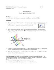
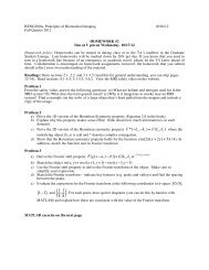
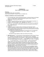
BENG280A, Principles of Biomedical Imaging 11/08/10
Fall Quarter 2010
Readings:
Read Chapters 6 and 7 in Nishimura
HOMEWORK #6
Due in Class on Thursday 11/18/10
Problems: (In Nishimura unless otherwise stated)
1. Problem 5.1
2. Problem 13.11 in Prince and Links.
3. Problem 5.6.
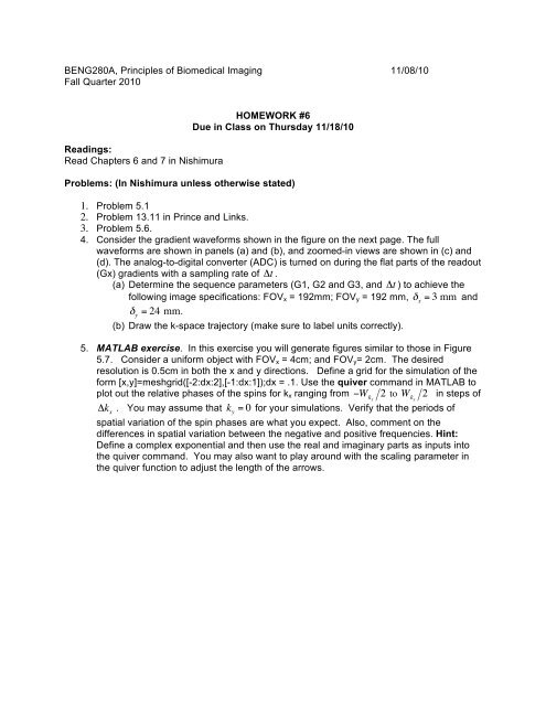
4. Consider the gradient waveforms shown in the figure on the next page. The full
waveforms are shown in panels (a) and (b), and zoomed-in views are shown in (c) and
(d). The analog-to-digital converter (ADC) is turned on during the flat parts of the readout
(Gx) gradients with a sampling rate of "t .
(a) Determine the sequence parameters (G1, G2 and G3, and "t ) to achieve the
following image specifications: FOV x = 192mm; FOV y = 192 mm, ! x
= 3 mm and
" y
= 24 mm.
!
(b) Draw the k-space trajectory (make sure to label units ! correctly).
!
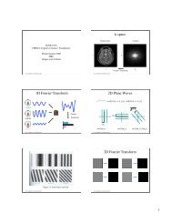
5. MATLAB exercise. In this exercise you will generate figures similar to those in Figure
! 5.7. Consider a uniform object with FOV x = 4cm; and FOV y = 2cm. The desired
resolution is 0.5cm in both the x and y directions. Define a grid for the simulation of the
form [x,y]=meshgrid([-2:dx:2],[-1:dx:1]);dx = .1. Use the quiver command in MATLAB to
plot out the relative phases of the spins for k x ranging from "W kx
2 to W kx
2 in steps of
"k x
. You may assume that k y
= 0 for your simulations. Verify that the periods of
spatial variation of the spin phases are what you expect. Also, comment on the
differences in spatial variation between the negative and positive frequencies. Hint:
Define a complex exponential and then use the real ! and imaginary ! parts as inputs into
the quiver command. ! You may also want to play around with the scaling parameter in
the quiver function to adjust the length of the arrows.

(a) Gx gradient
G1
0
-G1
(b) Gy gradient
G2
0
-G3
(c) Gx gradient (Zoomed in)
G1
0
T/2 = 320 usec
T = 640 usec
-G1
(d) Gy gradient (Zoomed in)
G2
! = 10 usec
0
-G3