Analog Electronics Basic Op-Amp Applications - LIGO

CALIFORNIA INSTITUTE OF TECHNOLOGY
PHYSICS MATHEMATICS AND ASTRONOMY DIVISION
Sophomore Physics Laboratory (PH005/105)
Analog Electronics
Basic Op-Amp Applications
Copyright c○Virgínio de Oliveira Sannibale, 2003
(Revision December 2012)

Chapter 5
Basic Op-Amp Applications
5.1 Introduction
In this chapter we will briefly describe some quite useful circuit based on
Op-Amp, bipolar junction transistors, and diodes.
5.1.1 Inverting Summing Stage
V 1
R
R f
V 2
V n
I2
In
I1
R
R
I
A
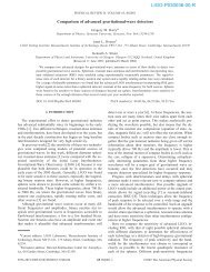
Figure 5.1: Inverting summing stage using an Op-Amp. The analysis of the
circuit is quite easy considering that the node A is a virtual ground.
Figure 5.1 shows the typical configuration of an inverting summing
stage using an Op-Amp. Using the virtual ground rule for node A and
107
−
+
I
V o
DRAFT

108 CHAPTER 5. BASIC OP-AMP APPLICATIONS
Ohm’s law we have
I n = V N
n
R , I = ∑ I n .
n=1
Considering that the output voltage V 0 is
V o = −R f I,
we will have
V o = A
N
∑
n=1
V n ,
A = − R f
R .
5.1.2 Basic Instrumentation Amplifier
Instrumentation amplifiers (In-Amp) are designed to have the following
characteristics: differential input, very high input impedance, very low
output impedance, variable gain, high CMRR, and good thermal stability.
Because of those characteristics they are suitable but not restricted to be
used as input stages of electronics instruments.
V i−
V i+
+
G
−
−
G
+
Input Stage
R 2
R 1
−
+
R 1
R 2
Differential
Stage
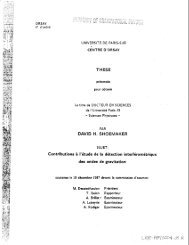
Figure 5.2: Basic instrumentation amplifier circuit.
Figure 5.2 shows a very basic In-Amp circuit made out of three Op-
Amps. In this configuration, the two buffers improve the input impedance
of the In-Amp, but some of the problems of the differential amplifier are
V o
DRAFT

5.1. INTRODUCTION 109
still present in this circuit, such as common variable gain, and gain thermal
stability.
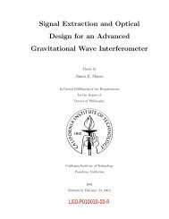
A straightforward improvement is to introduce a variable gain on both
amplifiers of the input stage as shown in Figure 5.3(a), but unfortunately,
it is quite hard to keep the impedance of the two Op-Amps well matched,
and at the same time vary their gain and maintaining a very high CMRR.
A clever solution to this problem is shown in Figure 5.3(b). Because of the
virtual ground, this configuration is not very different from the previous
one but it has the advantage of requiring one resistor to set the gain. In
fact, if R 3 = R 4 then the gain of the Op-Amps A 1 and A 2 can be set at the
same time adjusting just R G .
For an exhaustive documentation on instrumentation amplifiers consult
[2].
V i−
+
V i−
+
A 1 A 1
−
−
R 3
R G
R 4
R 2
−
−
A
V 2 A
i+ V 2
i+
R 1
+
+
R 3
R 4
(a)
Figure 5.3: Improved input stages of the basic instrumentation amplifier.
5.1.3 Voltage to Current Converter (Transconductance Amplifier)
A voltage to current converter is an amplifier that produces a current proportional
to the input voltage. The constant of proportionality is usually
called transconductance. Figure 5.4 shows a Transconductance Op-Amp,
which is nothing but a non inverting Op-Amp scheme.
(b)
DRAFT

110 CHAPTER 5. BASIC OP-AMP APPLICATIONS
i f
R Z f
R f
Z f
−
+
v (t)
s
Amperometer
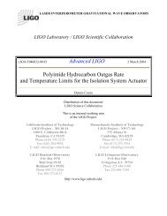
Figure 5.4: Basic transconductance amplifier circuit.
The current flowing through the impedance Z f is proportional to the
voltage v s . In fact, assuming the Op-Amp has infinite input impedance,
we will have
i f (t) = v s(t)
R .
Placing an amperometer in series with a resistor with large resistance
as a feedback impedance, we will have a high resistance voltmeter. In
other words, the induced perturbation of such circuit will be very small
because of the very high impedance of the operational amplifier.
5.1.4 Current to Voltage Converter (Transresistance Amplifier)
A current to voltage converter is an amplifier that produces a voltage proportional
to the input current. The constant of proportionality is called
transimpedance or transresistance, and its units are Ω. Figure 5.5 show a
basic configuration for a transimpedance Op-Amp. Due to the virtual
ground the current through the shunt resistance is zero, thus the output
voltage is the voltage difference across the feedback resistor R f , i.e.
v o (t) = −R f i s (t).
Photo-multipliers photo-tubes and photodiodes drivers are a typical
application for transresistance Op-amps. In fact, quite often the photocurrent
produced by those devices need to be amplified and converted
into a voltage before being further manipulated.
DRAFT

5.2. LOGARITHMIC CIRCUITS 111
i s
R f
−
i s
R s
+
v o =−i s R f
Figure 5.5: Basic transimpedance Op-Amp.
5.2 Logarithmic Circuits
By combining summing circuits with logarithmic and anti-logarithmic amplifiers
we can build analog multipliers and dividers. The circuits presented
here implements those non-linear operations just using the exponential
current response of the semiconductor junctions. Because of that,
they lack on temperature stability and accuracy. In fact, the diode reverse
saturation current introduces an offset at the circuits output producing a
systematic error. The temperature dependence of the diode exponential response
makes the circuit gain to drift with the temperature. Nevertheless
these circuits have a pedagogical interest and are the basis for more sophisticated
solutions. For improved logarithmic circuits consult [1] chapter 7,
and [1] section 16-13 and[3].
v
i
R
(a)
−
+
D
v
v i
o −
v o
Figure 5.6: Elementary logarithmic amplifiers using a diode or an npn BJT.
R
(b)
+
Q
DRAFT

112 CHAPTER 5. BASIC OP-AMP APPLICATIONS
5.2.1 Logarithmic Amplifier
Figure 5.6 (a) shows an elementary logarithmic amplifier implementation
whose output is proportional to the logarithm of the input. Let’s analyze
this non-linear amplifier in more detail.
The Op-Amp is mounted as an inverting amplifier, and therefore if v i
is positive, then v o must be negative and the diode is in conduction. The
diode characteristics is
)
i = I s
(e −qv o/k B T − 1 ≃ I s e −qv o/k B T
I s ≪ 1,
where q < 0 is the electron charge. Considering that
after some algebra we finally get
i = v i
R ,
v o = k BT
−q [ln(v i)−ln(RI s )] .
The constant term ln(RI s ) is a systematic error that can be measured
and subtracted at the output. It is worth to notice that v i must be positive
to have the circuit working properly. An easy way to check the circuit is to
send a triangular wave to the input and plot v o versus v i .
Because the BJT collector current I c versus V BE is also an exponential
curve, we can replace the diode with an npn BJT as shown in Figure 5.6.
The advantage of using a transistor as feedback path is that it should provide
a larger input dynamic range.
If the circuit with the BJT oscillates at high frequency, a small capacitor
in parallel to the transistor should stop the oscillation.
5.2.2 Anti-Logarithmic Amplifier
Figure 5.7 (a) shows an elementary anti-logarithmic amplifier, i.e. the output
is proportional to the inverse of logarithm of the input. The current
flowing through the diode is
i ≃ I s e −qv i/k B T
I s ≪ 1.
DRAFT

5.2. LOGARITHMIC CIRCUITS 113
R
R
v
i
D
−
Q
v
v i
o −
v o
+
+
(a)
(b)
Figure 5.7: Elementary anti-logarithmic amplifiers using a diode or an pnp BJT.
Considering that
thus
v o = −Ri ,
v o ≃ −RI s e −qv i/k B T .
If the input v i is negative, we have to reverse the diode’s connection. In
case of the circuit of Figure 5.7 (b) we need to replace the pnp BJT with an
npn BJT. Same remarks of the logarithmic amplifier about the BJT, applies
to this circuit.
v 1
v 2
Logarithmic
Amplifier
Logarithmic
Amplifier
R
R
−
+
Anti−Log
Amplifier
Figure 5.8: Elementary analog multiplier implementation using logarithmic and
anti-logarithmic amplifiers
R
v o
DRAFT

114 CHAPTER 5. BASIC OP-AMP APPLICATIONS
5.2.3 Analog Multiplier
Figure 5.8 shows an elementary analog multiplier based on a two log one
anti-log and one adder circuits. Fore more details about the circuit see [1]
section 7-4 and [1] section 16-13.
R
v 1
v 2
Logarithmic
Amplifier
Logarithmic
Amplifier
R
R
−
+
Anti−Log
Amplifier
v o
R 0
Figure 5.9: Elementary analog divider implementation using logarithmic and
anti-logarithmic amplifiers.
5.2.4 Analog Divider
Figure 5.8 shows an elementary logarithmic amplifier based on a two log
one anti-log and one adder circuits. Fore more details about the circuit see
[1] section 7-5 and [1] section 16-13.
5.3 Multiple-Feedback Band-Pass Filter
Figure 5.10 shows the so called multiple-feedback bandpass, a quite good
scheme for large pass-band filters, i.e. moderate quality factors around 10.
Here is the recipe to get it working. Select the following parameter
which define the filter characteristics, i.e the center angular frequency ω 0
the quality factor Q or the the pass-band interval (ω 1 , ω 2 ) , and the passband
gain A pb
DRAFT

R 2
R 0
5.3. MULTIPLE-FEEDBACK BAND-PASS FILTER 115
R 3
V i
C 1
R 1
C 2
−
V o
+
G
Figure 5.10: Multiple-feedback band-pass filter.
ω 0 = √ ω 2 ω 1
ω 0
Q =
ω 2 − ω 1
A pb < 2Q 2
Set the same value C for the two capacitors and compute the resistance
values
Verify that
R 1 =
R 2 =
R 3
Q
ω 0 CA pb
Q
ω 0 C(2Q 2 − A pb )
= 2Q
ω 0 C
A pb = R 3
2R 1
< 2Q 2
See [1] sections 8-4.2, and 8-5.3 for more details.
DRAFT

116 CHAPTER 5. BASIC OP-AMP APPLICATIONS
5.4 Peak and Peak-to-Peak Detectors
The peak detector circuit is shown in Figure 5.11. The basic ideal is to
implement an integrator circuit with a memory.
To understand the circuit letŽs first short circuit D o and remove R.
Then the Op-amp A 0 is just a unitary gain voltage follower that charges
the capacitor C up to the peak voltage. The function of D 0 and of A 1 (high
input impedance) is to prevent the fast discharge of the capacitor.
Because of D 0 the voltage across the capacitor is not the max voltage at
the input, and this will create a systematic error at the output v o . Placing
a feedback from v o to v i will fix the problem. In fact, because v + must be
equal to v − , A 0 will compensate for the difference.
Introducing the resistance (R ≃ 100kΩ) in the feedback will provide
some isolation for v o when v i is lower than v C .
The Op-Amp A 0 should have a high slew rate (~20 V/µs) to avoid the
maximum voltage being limited by the Op-Amp slew rate.
The capacitor doesn’t have to limit the Op-Amp A 0 slew rate S, i. e.
i C
C ≪ dv
dt = S
It is worthwhile to notice that if D 0 and D 1 are reversed the circuit
becomes a negative peak detector.
The technology of the hold capacitor C is important in this application.
The best choice to reduce leakage is probably polypropylene, and after
that polystyrene or Mylar.
Using a positive and a negative peak detector as the input of a differential
amplifier stage we can build a peak-to-peak detector (for more
details see [1] section 9-1). Some things to check: holding time (a given %
drop from the maximum) versus capacitor technology, systematic errors ,
settling time required for the output to stabilize.
5.5 Zero Crossing Detector
When v i is positive and because it is connected to the negative input then
v o becomes negative and the diode D 1 is forward biased and conducting.
DRAFT

5.6. ANALOG COMPARATOR 117
D 0
v C
v i
A
D 1
R
−
+
−
+
A
v o
C 0
RESET
Figure 5.11: Peak detector circuit.
5.6 Analog Comparator
An analog comparator or simply comparator is a circuit with two inputs v i ,
v re f and one output v o which fulfills the following characteristic:
{
V1 , v
v o =
i > v re f
V 2 , v i ≤ v re f
An Op-Amp with no feedback behaves like a comparator. In fact, if we
apply a voltage v i > v re f , then V + − V − = v i − v re f > 0. Because of the
high gain, the Op-Amp will set v o to its maximum value +V sat which is a
value close to the positive voltage of the power supply. If v i < v re f , then
v o = −V sat . The magnitude of the saturation voltage are typically about
1V less than the supplies voltages.
Depending on which input we use as voltage reference v re f , the Opamp
can be an inverting or a non inverting analog comparator.
It is worthwhile to notice that the analog comparator circuit is also a 1
bit analog digital converter , which converts voltages to the two levels V 1
and V 2 .
DRAFT

118 CHAPTER 5. BASIC OP-AMP APPLICATIONS
V i
V 1
−
+
V o
R +
R f
(utp)
V +
t
(ltp)
V +
+V sat
t
−V sat
Figure 5.12: Schmitt Trigger and its qualitative response to a signal that swings
up and down between and through the saturation voltages±V sat .
5.7 Regenerative Comparator (The Schmitt Trigger)
The Regenerative comparator or Schmitt Trigger 1 shown in Figure 5.12 is a
comparator circuit with hysteresis.
It is important to notice that the circuit has a positive feedback. With
positive feedback, the gain becomes larger than the open loop gain making
the comparator to swing faster to one of the saturation levels.
1 Otto Herbert Schmitt (1913-1998) American scientist considered the inventor of this
device, that appeared in an article in 1938 with the name of "thermionic trigger"[3].
DRAFT

5.8. PHASE SHIFTER 119
Considering the current flowing through R + and R f ,we have
I = V 1− V +
R +
= V +− V o
R f
, ⇒ V + = V 1R f + V o R +
R f + R +
.
The output V o can have two values, ±V sat . Consequently, V + will assume
just two trip points values
V (utp)
+ = V 1R f + V sat R +
R f + R +
V (ltp)
+ = V 1R f − V sat R +
R f + R +
When V i < V (utp)
+ , V o is high, and when V i < V (ltp)
+ , V o is low.
To set V + = 0 it requires that
V 1 = − R +
R f
V o
This circuit is usually used to drive an analog to digital converter (ADC).
In fact, jittering of the input signal due to noise which prevents from keeping
the output constant, will be eliminated by the hysteresis of the Schmitt
trigger (values between the trip points will not affect the output).
See [1] section 11 for more detailed explanations.
Example1: (V sat = 15V)
Supposing we want to have the trip points to be V + = ±1.5V, if we set
V 1 = 0 then R f = 9R + .
5.8 Phase Shifter
A phase shift circuit shown in Figure 5.13, produces a sinusoidal signal
at the output V o which is equal to the sinusoidal input V i with a defined
phase shift . The basic idea of this clever circuit is to subtract using an
Op-Amp two equal sinusoids one of which is lagging behind because is
low pass filtered (the difference of these two same frequency sinusoid is a
phase shifted attenuated sinusoid). The Op-Amp provides also the unitary
gain.
DRAFT

120 CHAPTER 5. BASIC OP-AMP APPLICATIONS
V i
R 0
R 0
−
+
V o
R
C
Figure 5.13: Phase shifter circuit.
Using the same method applied to compute the differential Op-Amp
stage transfer function, we obtain
H(ω) =
1− jωRC
1+ jωRC ,
The amplitude and phase of the transfer function are therefore
H(ω) = 1
for any frequency,
ϕ(ω) = arctan(−ωRC)− arctan(ωRC) = −2 arctan(ωRC) .
The phase shift is double the one of a simple low pass filter and therefore
can go from 0 ◦ down to −180 ◦ . Exchanging the potentiometer and
the capacitor changes the phase lag to a phase lead.
Example
Supposing that we want a phase shift of −90 ◦ for a 1 kHz sinusoid with
capacitor with a reasonable capacitance value C = 10 nF, then
R =
( ϕ
− tan
2)
Cω
=
1
10 −8· = 15.915 kΩ.
2π·103 The value of R 0 can be in the range of few kilohoms to tens kilohoms.
DRAFT

5.9. GENERALIZED IMPEDANCE CONVERTER (GIC) 121
5.9 Generalized Impedance Converter (GIC)
A
+
−
Z 1
Z 2
Z 3
+
−
Z 4
Z 5
A
Z
Figure 5.14: Generalized Impedance Converter (GIC).
The fundamental equation of the GIC, which can be found after tedious
calculation, is
Z = Z 1Z 3 Z 5
Z 2 Z 4
By a careful choice of passive components, one can implement types
of impedance with values impossible to attain with standard passive components.
This holds true where the Op-Amps behave very closely to ideal
Op-Amps and if one lead of Z is grounded. For example, we can make:
• C to L converter and vice versa,
• LC parallel to LC series and vice versa,
• impedance scaler
• negative resistance
DRAFT

122 CHAPTER 5. BASIC OP-AMP APPLICATIONS
This circuit is also a gyrator, i.e. a two voltage controlled current sources,
where the currents have opposite direction. For more details consult [7].
5.9.1 Capacitor to Inductor Converter
If we choose, for example,
then the GIC becomes
Z 1 = Z 2 = R 1 , Z 3 = R 3 , Z 4 = 1
jωC , Z 5 = R 5 ,
Z = jωR 3 R 5 C .
The circuit will behave as an inductor with inductance L = R 3 R 5 C. If
we chose large resistance values R 3 , R 5 and reasonably large capacitance
values C, we can implement very large inductance values practically impossible
to attain using standard inductors.
DRAFT

5.10. PROBLEMS PREPARATORY TO THE LABORATORY 123
5.10 Problems Preparatory to the Laboratory
1. Considering the following circuit, determine the voltage output V o
for the following input voltages V i = −2V, 1V, 1.5V, 3V
+10V
V i
+1.5V
−
+
G
V o
−10V
2. Consider the Schmitt trigger of Figure 5.12.
(a) If V o = −15V and V + = 0V, compute V 1 .
(b) If V o = +15V, and V 1 = 15V, compute V + .
3. Design a Schmitt trigger with two diode clamps and one resistor connected
to the output.
(a) Limit the output V o from 0 to 5V.
(b) Compute the resistance value R necessary to limit the diode current
to 10mA.
4. What is the practical maximum and minimum output voltage of the
logarithmic amplifier in Figure 5.6?
5. Chose and study at least two circuits to study and design, one from
this chapter and one form the next one on active filters .
New circuits different than those ones proposed in this chapter are
also welcome. For a good source of new circuits based on Op-Amps
see [1] , [4], and [2].
DRAFT

124 CHAPTER 5. BASIC OP-AMP APPLICATIONS
DRAFT

Bibliography
[1] Luces M. Faulkenberry, An introduction to Operational Amplifiers
with Linear IC Applications, Second Edition.
[2] Charles Kitchin and Lew Counts, A Designer’s Guide to
Instrumentation Amplifiers (2nd Edition), Analog Devices
(http://www.analog.com/en/DCcList/0,3090,759%255F%255F42,00.html)
[3] Theory and Applications of Logarithmic Amplifiers, National
Semiconductors, AN-311 ( http://www.national.com/an/AN/AN-
311.pdf ).
[4] Horowitz and Hill, The Art of Electronics, Second Edition
[5] Microelectronics Jacob Millman & Arvin Grabel, McGraw-Hill Electrical
Engineering Series
[6] A thermionic trigger, Otto H Schmitt 1938 J. Sci. Instrum. 15 24-26.
[7] Sedra Smith, Microelectronics Circuits, third edition, Oxford University
Press.
125
DRAFT

126 BIBLIOGRAPHY
DRAFT