A Program for Calculating the Montgomery Stream Function

A PROGRAM FOR CALCULATING THE MONTGOMERY STREAM FUNCTION
Erwin T. Prater*
University of Wyoming
Laramie, Wyoming
Abstract
Many current upper-air analysis packages peiform isentropic
analysis. However, some of those packages do not calculate
the MontgomelY stream function (M) on isentropic suifaces.
This may make it difficult to accurately determine ageostrophic
forcing from differences between geostrophic and total winds
since geostrophic winds are proportional to gradients of M on
isentropic sUifaces. Starting from theory, this paper derives an
approach for finding M from isobaric data. The approach is
then translated into a FORTRAN program which computes M.
For illustrative purposes, the program processes user-supplied
upper-air data. Two data sets are provided to help the user
test resulting code. Meteorologists could adapt the code for
inclusion in upper-air or gridded-data analysis packages which
do not currently calculate M. The author has regularly used
the code to produce isentropic analyses since 1993.
1. Introduction
There are a number of programs which analyze upper-air
observations and gridded model output. Many of these programs
include some level of isentropic analysis. However, some
of those programs (e.g., PCGRIDDS) (NWS 1994) do not calculate
the Montgomery stream function (M = CpTo + gzo) (Montgomer~
I ?37) on isentropic surfaces. M is crucial to isentropic
analYSIS SInce geostrophic wind speeds on isentropic surfaces
are proportional to gradients of M. (M performs a role on
isentropic surfaces which is analogous to geopotential height
on isobaric surfaces.) Some cunent isentropic analysis packages
(e.g., PCGRIDDS) determine geostrophic winds on isentropic
surfaces by interpolating them from isobaric surfaces. While
this may outwardly appear to be a reasonable procedure, it
does not guarantee that the resulting geostrophic winds are as
accurate, or as representative, as they could be. Problems with
geostrophic winds affect ageostrophic winds derived from vector
differences between geostrophic and total winds.
Starting from theory, this paper derives an approach for
finding M from isobaric data. The approach is translated into
a FORTRAN program which computes M. For illustrative purposes,
the program is set up to process user-supplied upper-air
data. Two data sets are provided to help the user test resultino
code. In principle, the program could be adapted for use i~
upper-air or gridded-data analysis packages which do not calculate
M. Meteorologists familiar with macros may be able to
translate the program into a macro provided that the analysis
package of interest allows the user to find the nearest isobaric
suifaces above and below an isentropic suiface of interest. Not
all analysis packages allow this. The paper proceeds as follows.
The mathematical basis of the program is developed in section
2. The results of the program from two data sets are given in
section :3'". Section 4 summarizes the results. The program and
data sets are given in the Appendix.
2. Mathematical Basis of the Program
In the 1930s, upper-air analyses were performed on constantaltitude,
isobaric and isentropic (6) surfaces. At that time the
merits of each type of chart were actively debated. Debate
continued and by the end of World War II, isobaric charts were
routinely analyzed by forecasters in the U.S. Weather Bureau
(WB) (Fulks 1945). Isentropic analysis was not regularly performed
again until the 1950s and 1960s.
One. possib~e reason for the temporary demise of isentropic
analYSIS was maccurate Montgomery stream functions which
resulted in geostrophic wind laws which did not appear to work
on isentropic charts (Bleck 1973; Moore 1988). In retrospect,
Brooks (1942) almost found the reason for those inconect
comput~t~ons. He observed that CpTo and gzo varied inversely
and Indl~ldually much faster than their sum M = CpTo + gzo,
so that In terms of numerical accuracy, it was desirable to
calculate a small quantity M' defined as M' = M - CpO rather
than M. However, it was Danielsen (1959) who discovered the
actual reason for the inconect computations. He noted that the
WB had incorrectly calculated M. They separately interpolated
Zo a~d .To in t~e two terms which comprise M and thereby
~nwlttlllgly VIOlated hydrostatic consistency constraints
Imposed on each term. Using Danielsen's work, Mahlman and
Kamm (1965) (henceforth, MK65) and later Reiter (1972) prop.osed
and tested a method of calculating M whose accuracy
nvaled standard methods of determining geopotential height
along isobaric surfaces. This method wiII be the basis for the
program in the Appendix. MK65 started with the total differential
of M
which becomes
dM = CpdTo + gdzo (2)
after substituting the definition of M for the partial derivatives
!n (1) .and neglecting higher-order terms. An expression for dzo
IS denved from the hypsometric equation,
RT I (Pe)
Zo = Ze + g n Po (3)
*Current affiliation: Trinity Consultants, 12801 N. Central Expressway, Suite 1200, Dallas, Texas 75243.
53
J

S4
National Weather Digest
whose total differential is
dzo = d z +-n- R I (Pe) d-T +-- RT dP e
e g Po g P e
_ RT dPo + HOT
g Po
Danielsen substituted (4) into (2) and neglected higher-order
terms (HOT) to produce
dM = gdze + R In (~:) if + iT~e
- dP e
- RT - + CpdTo.
Po
He assumed that the differentials represent err..Qrs so that
(4)
11M = gLlz e + R In (P e ) I1T + RT !1.P e (6)
Po P e
+ [- RT I1P o + CpLlTo]
Po
where 11M is the error made if height>-pressure and temperature
of an isentropic surface (Zo.p o. To) and Tare determined independently
of each other.
Danielsen noted that an expression analogous to (6) for geopotential
height along an isobaric surface is derived from the
total differential of

Volume 20 Number 3 March, 1996
55
(4) Determine T from the average of To and Tb
T = Tb + To
2
(19)
(5) Substitute results from steps (1)-(4) into (17) to find M.
These steps can be translated into common computer languages,
or encoded as a macro in upper-air and gridded-data
processing packages which allow the user to find the nearest
isobaric sUlfaces above and below an isentropic suiface of
interest. A simple FORTRAN program which computes M is
shown in the Appendix. If the comments are removed, the
program is very short and easily typed with a text editor or
word processor. The program assumes that the user has information
from isobaric surfaces above and below the isentropic
surface of interest. In practice this information would likely be
contained in arrays so that the user would reference array elements
instead of READ statements (or other language-specific
input statements). Input isobaric data and M for two analyses
along the 319.5 K isentropic surface are given in Tables 1
and 2 in the Appendix. The data are taken from 3-h CLASS
radiosonde observations at 2100 UTC 8 March 1992 - 0000
UTC 9 March 1992 during STORM-FEST (STormscale Operational
and Research Meteorology-Fronts Experiment Systems
Test) (Cunning and Williams 1993). As part of STORM-FEST,
flow along the 319.5 K isentropic surface was followed by
an instrumented aircraft (Prater 1994) during lee cyclogenesis
(Mahoney et al. 1995).
3. Results
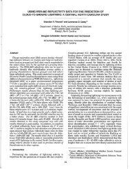
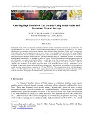
Figure 1 shows M (thick lines), geostrophic wind isotachs
(thin, dashed lines), pressure (thin, solid lines) and observed
winds on the 319.5 K isentropic surface at 2100 UTC 8 March
1992. M was computed using the first data set in the Appendix.
M was contoured at a 1200 m 2 S - 2 interval to aid comparison
with height on isobaric charts contoured at a 120 m interval.
The figure shows a trough over the southern Rockies and the
exit region of a jet. Observed wind speeds over southern New
Mexico and west Texas are sub-geostrophic, as expected in
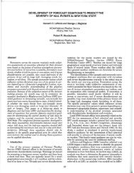
cyclonically-curved flow. In the operational environment, the
quality of an isentropic analysis is often assessed by comparing
it with a nearby isobaric surface. That approach will be used
here. Height, geostrophic wind isotachs and observed winds on
the nearby 320-mb isobaric surface are shown for comparison in
Fig. 2. Figures 1 and 2 show reasonable qualitative agreement
between the pressure gradient fields and geostrophic wind
speeds, with exception of southwest Texas where the 319.5 K
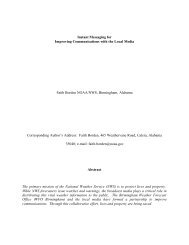
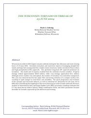
isentropic surface was closer to 400 mb. Another example of
M on the 319.5 K isentropic surface from the program at 0000
UTC 9 March 1992 (the second data set in the Appendix) is
shown in Fig. 3. This analysis shows good time continuity with
Fig. 1, with eastward motion of the trough and northeastward
propagation of the jet streak. Analysis of the nearby 320-mb
8640 20----.
320 mh
2100 UTe
08 March 1992
Fig. 2. 320-mb isobaric analysis at 21 00 UTe 8 March . Height (thick
lines and meters); observed winds (m s- ') (same barb convention
as in Fig. 1); geostrophic wind isotachs (dashed lines and m s- ')
319.5 K
2100 UTe
08 March 1992
Fig. 1. The 319.5 K isentropic surface at 2100 UTe 8 March 1992.
M computed from the program (thick lines and m 2 s -2); isobars (thin
lines and mb); observed winds (m s- '); full barb = 10 m s- '; flag
= 50 m s-'; geostrophic wind isotachs (dashed lines and m s- ').
'-..40~
319.5 K
0000 UTe
09 March 1992
Fig. 3. Same as Fig. 1 except 0000 UTe 9 March 1992.

56
National Weather Digest
8820
~ __-:-r-'
Service Training Center in Kansas City which the author had the
pleasure of attending several years ago. The author's research
at UW was supported by National Science Foundation grant
ATM-9308409.
Author
320 mb
0000 UTe
09 March 1992
Fig. 4. Same as Fig. 2 except 0000 UTe 9 March 1992.
isobaric surface is shown in Fig. 4 for comparison. Figures 3
and 4 show reasonable qualitative agreement with exception
of eastern Oklahoma and Texas where the 319.5 K isentropic
surface was closer to the 400-mb level. Although only two
isentropic analyses are presented, both show reasonable consistency
with analyses on nearby isobaric surfaces. Other examples
of M computed using a similar approach and isobaric surfaces
are shown by Reiter (1972). The author has used the program
in the Appendix since 1993 to regularly generate M using an
upper-air analyses package adapted from MK65.
4. Summary
There are a number of programs which analyze upper-air
observations and gridded model output. Many programs include
some level of isentropic analysis. However, some of those
programs (e.g., PCGRIDDS) do not analyze the Montgomery
stream function (M) on isentropic surfaces. Starting from theory,
this paper presented an approach for finding M from isobaric
data. The approach was translated into a FORTRAN
program which computes M. For illustrative purposes, the program
is set up to process user-supplied upper-air data. Two
isentropic analyses featuring M from the program were shown.
Those analyses showed good time continuity and reasonable
qualitative agreement with features on nearby isobaric surfaces.
The author has used the program successfully since 1993 in an
upper-air analyses package adapted from MK65. Meteorologists
are encouraged to test and refine the program, and implement
the code in PCGRIDDS and other upper-air analysis
packages which do not calculate M.
Acknowledgments
The author wishes to thank Drs. John D. Marwitz and Thomas
R. Parish of the University of Wyoming (UW) for their assistance.
This work was derived from a very small part of the
author's dissertation at UW. The author also thanks Ms. Susan
Allen at UW for drafting the figures. The author is indebted
to Dr. James T. Moore of St. Louis University and one other
(anonymous) reviewer for their comments. Dr. Moore also
teaches a course on isentropic analysis at the National Weather
Dr. Erwin T. Prater is currently employed with Trinity Consultants,
Inc. of Dallas, Tx. His work with Trinity concerns airquality
and chemical hazard analyses. He holds M.S. and Ph.D.
degrees in Atmospheric Science from the University of Wyoming.
He has been employed by the NWS, NASA and the
Soil Conservation Service. He has also been a private-sector
consultant in forensic meteorology and computational fluid
dynamics. His professional interests vary widely from aircraft
icing and freezing rain, in airborne dynamical studies, to dispersion
modeling and boundary-layer meteorology. Dr. Prater is
currently vice-president of the Arkansas NW A chapter.
References
Bleck, R., 1973: Numerical Forecasting Experiments Based on the
Conservation of Potential Vorticity on Isentropic Surfaces. 1. Appl.
Meteor., 12,737-752.
Brooks, E.M., 1942: Simplification of the Acceleration Potential
in an Isentropic Surface. Bull. Amer. Meteor. Soc., 23, 195-203.
Cunning, J., and S. Williams, 1993 STORM-FEST Operations
Summary and Data Inventory. [Available from UCAR Office of
Field Project Support, P.O. Box 3000, Boulder, CO 80307.]
Danielsen, E.F., 1959: The Laminar Structure of the Atmosphere
and its Relation to the Concept of a Tropopause. Arch. Meteor.
Geophys., All, 293-332.
Fulks, 1.R., 1945: Constant Pressure Maps-Methods of Preparation
and Advantages in their Use. Bull. Amer. Meteor. Soc., 26,
133-146.
Mahlman, J.D., and W. Kamm, 1965: Development of Computer
Programs for Computation of Montgomery Stream Functions and
Plotting Thermodynamic Diagrams. Atmospheric Science Technical
Paper No. 70., pp. 122-145, Colorado State University. [Available
from the Department of Atmospheric Science, Colorado State
University, Fort Collins, CO.]
Mahoney, 1.L., J.M. Brown and E.!. Tollerud, 1995: Contrasting
Meteorological Conditions Associated with Winter Storms at Denver
and Colorado Springs. Wea. Forecasting, 10, 245-260.
Montgomery, R.B., 1937: A Suggested Method for Representing
Gradient Flow in Isentropic Surfaces. Bull. Amer. Meteor. Soc.,
18,210-212.
Moore, J.T., 1988 Isentropic Analysis and Interpretation: Operational
Applications to Synoptic and Mesoscale Forecast Problems.
[Available from the National Weather Service Training Center,
Kansas City, Missouri.]
National Weather Service, 1994: PCGRIDDS User's Manual. 121
93 version. [Available from National Weather Service Training
Center.]
Prater, E. T., 1994: Aircraft Measurements of Ageostrophic Winds.
Ph.D. Dissertation, Department of Atmospheric Science, University
of Wyoming. 288 pp.
Reiter, E.R., 1972: Atmospheric Transport Processes. Part 3:
Hydrodynamic Tracers. TID 25731. [Available from the National
Technical Information Service, Springfield, VA.]

Volume 20 Number 3 March, 1996 57
APPENDIX: PROGRAM AND DATA
C*************************************************
C*************************************************
PROGRAM MONT
C MONT.FOR
C
C
REAL SURF,TTHETA,TA,TB,TBAR,M,R,CP
C THIS CODE ILLUSTRATES A PROGRAM FOR COM-
CHARACTER*3 STAT
C PUTING THE WONTGOMERY STREAM FUNCTION.
INTEGER IMAX
C
C WRITTEN BY ERWIN T. PRATER AUGUST, 1993 FOR C GAS CONSTANTS (MKS UNITS)
C UPPER-AIR ANALYSIS
R=287.04
C CP= 1004.6
C WRITTEN AND COMPILED ON AN IBM-COMPATI-
C BLE 486DX2 USING MICROSOFT FORTRAN 77. CODE
C BASED ON MAHLMAN AND KAMM (65).
C GRAVITATIONAL CONSTANT (MKS UNITS)
C
G=9.806
C*************************************************
C C SPECIFY THE ISENTROPIC SURFACE OF
C VARIABLES ENTERED BY THE USER: C INTEREST AND COLLECT INFORMATION
C C ABOUT NEARBY ISOBARIC SURFACES.
C STAT = THREE-LETTER STATION ID
C
WRITE(*,*) 'ENTER THE TEMPERATURE (K) OF
C SURF = ISENTROPIC SURFACE OF INTEREST THE THETA SURFACE'
C (KELVIN) READ(*,*) SURF
C
C TA = TEMPERATURE OF THE NEAREST C 1M AX SPECIFIES THE NUMBER OF LOCATIONS
C ISOBARIC SURFACE ABOVE THE C WHERE THE MONTGOMERY STREAM FUNC-
C ISENTROPIC SURFACE (CELSIUS) C TION WILL BE CALCULATED. IMAX IS SET TO
C C 9 IN THIS PROGRAM. IN PRACTICE IT HAS NO
C TB = TEMPERA TURE OF THE NEAREST C PRACTICAL LIMIT.
C
ISOBARIC SURF ACE BELOW THE
C ISENTROPIC SURFACE (CELSIUS)
C
IMAX=9
DO 2 1= I,1MAX
WRITE(*,*) 'ENTER THE THREE-LETTER STA-
C TROPIC SURFACE (MILLIBARS) TION IDENTIFIER'
C
READ(*,I) STAT
C PB = PRESSURE OF THE NEAREST ISO- FORMAT (A3)
C
BARIC SURFACE BELOW THE ISEN-
C
C
PA = PRESSURE OF THE NEAREST ISO-
BARIC SURFACE ABOVE THE ISEN-
C TROPIC SURFACE (MILLIBARS) WRITE(*,*) ' ENTER THE TEMPERATURE (C)
C
AND PRESSURE'
C ZB = GEOMETRIC ALTITUDE OF AN ISO- WRITE(*,*) '(MB) OF THE CLOSEST ISOBARIC
C BARIC SURFACE BELOW THE ISEN- SURFACE ABOVE'
C TROPIC SURFACE (METERS) WRITE(*,*) ' THE ISENTROPIC SURFACE OF
C
INTEREST'
C INTERNALLY-COMPUTED VARIABLES:
READ(*,*) TA,PA
C
TA=TA+273.15
C 1M AX = NUMBER OF LOCATIONS WHERE M
C IS COMPUTED WRITE(*,*) 'ENTER HEIGHT, TEMP. (C) AND
C
PRESSURE'
C TTHET A = TEMPERATURE OF THE ISENTROPIC
WRITE(*,*) '(MB) OF THE CLOSEST ISOBARIC
C
SURFACE
SURFACE BELOW'
C
WRITE(*,*) ' THE ISENTROPIC SURFACE OF
C THET AA = POTENTIAL TEMPERATURE OF THE
INTEREST'
C
ISOBARIC SURFACE ABOVE THE
READ(*,*) ZB,TB,PB
C
ISENTROPIC SURFACE OF INTEREST
TB =TB + 273.15
C
C THET AB = POTENTIAL TEMPERATURE OF THE
C
ISOBARIC SURFACE BELOW THE C COMPUTE THE TEMPERATURE OF THE ISEN-
C ISENTROPIC SURFACE OF INTEREST C TROPIC SURFACE OF INTEREST (TTHETA)
C
C TBAR = MEAN TEMPERATURE BETWEEN PB THETAA = TA*((1000.IPA)**(RlCP))
C AND THE ISENTROPIC SURFACE THETAB = TB *((lOOO.IPB)**(RlCP))
C (KELVIN) TTHETA = TB +(TA-TB)*((SURF-THE
C
TAB )/(THET AA -THET AB))
C M = MONTGOMERY STREAM FUNCTION
C (m**2/s**2) C COMPUTE THE MEAN TEMPERATURE (TBAR)
C C BETWEEN THE ISENTROPIC SURFACE OF

58
National Weather Digest
C
C
C
C
C
&
INTEREST AND THE ISOBARIC SURFACE
BELOW
TBAR = (TTHETA+TB)I2.
COMPUTE M
M=CP*TTHETA + G*ZB + R*TBAR*
ALOG((PBIlOOO.)*((SURF/TTHETA)**(CPI
R)))
WRITE THE COMPUTED M AND STATION ID
WRITE(*,*) 'STATION ', ' MONT. SFN.
(m**2/s**2): '
WRITE(*,3) STAT,M
3 FORMAT (A4,8X,F8.0)
2 CONTINUE
STOP
END
LIST OF SYMBOLS
a, b subscripts for variables above and below a specific
level, respectively
Cp specific heat of dry air at constant pressure
(1004.6 J kg-I K- 1 )
e subscript denoting the Earth's surface
g gravitational constant (9.806 m S-2)
M Mon~gomery stream function (M = CpTo + gzo)
M' modified Montgomery stream function
P pressure; subscript for an isobaric surface
geopotential height
R dry gas constant (287.04 J kg-I K- 1 )
T absolute temperature
- T mean absolute temperature
e potential temperature; subscript for an isentropic
surface
z geometric altitude
Table 1. Input data and M 2100 UTC 8 March 1992. M is contoured in Fig. 1.
Temperature
Height (m),
Station and (0C) and temperature and
three-letter pressure (mb) pressure below
identifier above 9=319.5K 9=319.5K M (m2 S-2)
Topeka, KS (TOP) -50.7 280 9493 -49.0 290 318438
Arkansas City, KS (AKZ) -38.0 340 8244 -36.4 350 318630
Dodge City, KS (DOC) -48.7 290 9236 -47.4 300 318108
Guymon, OK (GUY) -44.0 310 8796 -42.2 320 318031
Albuquerque, NM (ABO) -38.9 330 8212 -39.7 340 316352
Amarillo, TX (AMA) -37.3 340 8199 -36.7 350 318189
Norman, OK (OUN) -38.1 340 8255 -36.6 350 318739
EI Paso, TX (ELP) -32.4 370 7588 -30.9 380 317851
Midland, TX (MAF) -33.4 360 7867 -32.6 370 318739
Table 2. Input data and M 0000 UTC 9 March 1992. M is contoured in Fig. 3.
Temperature
Height (m),
Station and (0C) and temperature and
three-letter pressure (mb) pressure below
identifier above 9 = 319.5K 9=319.5K M (m2 S-2)
Topeka, KS (TOP) -40.2 330 8426 -38.6 340 318453
Hays, KS (HYS) -48.5 290 9228 -46.9 300 318033
Dodge City, KS (DOC) -53.0 270 9647 -51.2 280 317700
Guymon, OK (GUY) -40.0 330 8342 -38.4 340 317630
Albuquerque, NM (ABO) -42.4 310 8599 -43.0 320 316100
Amarillo, TX (AMA) -34.3 360 7760 -33.0 370 317689
Norman, OK (OUN) -34.0 360 7838 -32.7 370 318455
EI Paso, TX (ELP) -38.1 340 8159 -36.6 350 317796
Midland, TX (MAF) -32.2 370 7660 -30.9 380 318557