gravity waves, unbalanced flow, and aircraft clear air turbulence (1)
gravity waves, unbalanced flow, and aircraft clear air turbulence (1)
gravity waves, unbalanced flow, and aircraft clear air turbulence (1)

You also want an ePaper? Increase the reach of your titles
YUMPU automatically turns print PDFs into web optimized ePapers that Google loves.
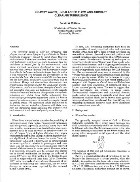
GRAVITY WAVES, UNBALANCED FLOW, AND AIRCRAFT<br />
CLEAR AIR TURBULENCE<br />
Donald W. McCann<br />
NOAA/National Weather Service<br />
Aviation Weather Center<br />
Kansas City, Missouri<br />
Abstract<br />
The "accepted" cause of <strong>clear</strong> <strong>air</strong> <strong>turbulence</strong> that<br />
plagues <strong><strong>air</strong>craft</strong> when flying at high altitudes is Kelvin<br />
Helmholtz instability caused by wind shear. However,<br />
environmental Richardson numbers associated with <strong><strong>air</strong>craft</strong><br />
<strong>turbulence</strong> reports are too high to assume that the<br />
<strong>turbulence</strong> is caused just by the environmental wind<br />
shear. Forecast techniques developed to date have<br />
assumed that there are layers of local Richardson number<br />
favorable for <strong>turbulence</strong> within the larger layer for which<br />
it was measured. The forecasts are probabilistic in the<br />
sense that the lower the environmental Richardson number,<br />
the more likely somewhere in the layer there will be<br />
<strong>turbulence</strong>. Theory <strong>and</strong> observations demonstrate that<br />
<strong>gravity</strong> <strong>waves</strong> can locally modify the wind shear <strong>and</strong> stability<br />
so as to produce <strong>turbulence</strong>. Analysis of model output<br />
associated with <strong>clear</strong> <strong>air</strong> <strong>turbulence</strong> events suggests<br />
that <strong>turbulence</strong> <strong>and</strong> indicators of large-scale atmospheric<br />
imbalance are related. Since highly <strong>unbalanced</strong> <strong>flow</strong><br />
must undergo geostrophic adjustment which is a known<br />
cause of <strong>gravity</strong> <strong>waves</strong>, <strong>clear</strong> <strong>air</strong> <strong>turbulence</strong> may be caused<br />
by <strong>gravity</strong> <strong>waves</strong>. The conclusion, while preliminary, is<br />
that better <strong>clear</strong> <strong>air</strong> <strong>turbulence</strong> forecasts will likely come<br />
from an ingredients-based technique that includes both<br />
environmental wind shear <strong>and</strong> <strong>gravity</strong> wave forcing.<br />
1. Introduction<br />
Pilots have always had to consider the possibility of<br />
<strong>turbulence</strong> along their routes. Pilots expect <strong>turbulence</strong><br />
near the ground, especially on windy, sunny days, <strong>and</strong><br />
near weather systems such as fronts that produce phenomena<br />
such as rain showers or thunderstorms. As<br />
<strong><strong>air</strong>craft</strong> began flying at higher altitudes, they began<br />
encountering <strong>turbulence</strong> unexpectedly in regions without<br />
significant cloudiness, hence the name "<strong>clear</strong> <strong>air</strong><br />
<strong>turbulence</strong>." CAT, as it is known, can be strong enough<br />
to cause significant injuries to passengers <strong>and</strong> crew<br />
when it is not expected. The news media has reported<br />
several of these events in recent years. However, when<br />
it is expected, occupants can be secured <strong>and</strong> objects<br />
can be stowed to minimize the damage. An outbreak of<br />
severe CAT over the Ohio Valley in the United States<br />
lasted an unprecedented three days (12-14 December<br />
1997) with hundreds of <strong><strong>air</strong>craft</strong> <strong>and</strong> thous<strong>and</strong>s of <strong>air</strong><br />
travelers encountering the <strong>turbulence</strong>, yet no major<br />
damage or injuries were reported by the national<br />
media (Cundy 1999).<br />
To date, CAT forecasting techniques have been an<br />
amalgamation of mostly empirical rules <strong>and</strong> equations<br />
(Dutton 1980; Knox 1997), most of which are based on<br />
connections between observed atmospheric patterns <strong>and</strong><br />
<strong><strong>air</strong>craft</strong> <strong>turbulence</strong> reports. Doswell et al. (1996) summarized<br />
current thunderstorm forecasting techniques as<br />
being "ingredients-based." Simply put, there needs to be<br />
a favorable environment <strong>and</strong> a triggering mechanism in<br />
place for a thunderstorm to develop. This paper outlines<br />
a similar ingredients-based technique for CAT forecasting.<br />
The environmental setup can be measured by the<br />
vertical wind shear <strong>and</strong> the Richardson number. The triggers<br />
are <strong>gravity</strong> <strong>waves</strong>. While the technique is largely<br />
theoretical, reports from a CAT pilot report database are<br />
compared with diagnostics of wind shear <strong>and</strong> Richardson<br />
number <strong>and</strong> with diagnostics of <strong>unbalanced</strong> <strong>flow</strong>, a<br />
known cause of <strong>gravity</strong> <strong>waves</strong>. The results suggest that<br />
these ingredients are present in many cases.<br />
Environmental observations <strong>and</strong> numerical forecast<br />
model output is adequate to quantifY wind shear <strong>and</strong><br />
Richardson number. Much less is known about <strong>gravity</strong><br />
<strong>waves</strong> produced from <strong>unbalanced</strong> <strong>flow</strong>. Quantifying this<br />
triggering mechanism requires much more theoretical<br />
<strong>and</strong> observational research.<br />
2. Background<br />
a. Richardson number<br />
The generally accepted cause of CAT is Kelvin<br />
Helmholtz instability (KHI) which occurs between two<br />
fluid layers that are statically stable but have sufficiently<br />
different velocities. The Richardson number is the ratio<br />
of static stability, as measured by the Brunt-Vaisala frequency<br />
(often designated as N) squared, <strong>and</strong> the wind<br />
shear squared:<br />
The notation of this <strong>and</strong> all subsequent equations is<br />
defined in the appendix. '<br />
There is a special relationship of <strong>turbulence</strong> to the Ri.<br />
Because the denominator is always positive, when the<br />
stability is negative, i.e., the lapse rate is superadiabatic,<br />
Ri < 0.0 <strong>and</strong> convective <strong>turbulence</strong> can develop. When 0.0<br />
< Ri < 0.25, KHI can form, <strong>and</strong> when Ri > 0.25, KHI cannot<br />
form. This critical Richardson number can be shown<br />
(1)<br />
3
J<br />
4<br />
National Weather Digest<br />
theoretically (Miles <strong>and</strong> Howard 1964) <strong>and</strong> experimentally<br />
(Thorpe 1969) as a threshold below which an atmosphere<br />
may be turbulent. Stabilities <strong>and</strong> wind shears as<br />
measured by st<strong>and</strong>ard rawinsonde observations yielding<br />
Richardson numbers less than 0.25 are common in the<br />
boundary layer (McCann 1999). Above the boundary<br />
layer where CAT occurs, Ri values less than 0.25 have<br />
been observed in thin layers by special observations<br />
(Browning et al. 1970; Reed <strong>and</strong> Hardy 1972) but are<br />
rarely observed by st<strong>and</strong>ard rawinsondes (Murphy et al.<br />
1982). Because layers with Ri < 0.25 should quickly<br />
become turbulent <strong>and</strong> raise Ri to more stable values, it is<br />
by chance when a rawinsonde observes one.<br />
Numerous researchers in the 1960s <strong>and</strong> early 1970s<br />
recognized that customary atmospheric observations<br />
were too coarse to observe the stabilities <strong>and</strong> wind shears<br />
that result in low Ri values <strong>and</strong> CAT. As a group, they<br />
made an implicit assumption that the lower the environmental<br />
Richardson number (RiE), the more likely that<br />
somewhere within that thick layer, there were thin layers<br />
of local Richardson number (Ri L less than the critical<br />
value (e.g., Roach 1970). Since in many cases it was high<br />
environmental wind shear that lowered RiE, quoting from<br />
Knox (1997b), ''The mystery of CAT was thought to be<br />
solved when its connection to vertical shear instabilities<br />
was discovered (Dutton <strong>and</strong> Panofsky 1970)." Forecast<br />
techniques from that era stressed analysis of RiE, especially<br />
the vertical wind shear portion. For example, Roach<br />
(1970) derived a RiE tendency equation. Even the more<br />
recent Ellrod <strong>and</strong> Knapp (1992) index of wind shear times<br />
deformation is wind shear-based. Frontogenetic deformation<br />
can cause the large-scale wind shear to increase<br />
through the thermal wind relationship, <strong>and</strong> it was the<br />
rationale in including it in their index. Knox (1997b) analyzed<br />
the theory underlying these methods <strong>and</strong> found it<br />
incomplete since other dynamic processes can also<br />
increase environmental wind shear.<br />
b. Turbulent kinetic energy<br />
Turbulent kinetic energy (TKE) equations are the<br />
basis for underst<strong>and</strong>ing <strong>turbulence</strong> in the atmospheric<br />
boundary layer (McCann 1999). Since they are based on<br />
the equations of motion, they should also be applicable to<br />
the free atmosphere. The simplest is a steady-state first<br />
order closure equation in which the <strong>turbulence</strong> is<br />
assumed to be analogous to diffusion, i.e., the turbulent<br />
flux of any quantity is proportional to the mean gradient<br />
of the quantity being transferred (Garratt 1992):<br />
This relationship is known as the flux-gradient TKE<br />
equation or K-closure equation because of the proportionality<br />
constants Km <strong>and</strong> Kh. The term on the left-h<strong>and</strong><br />
side of (2) is the TKE dissipation due to molecular viscosity<br />
while the two terms on the right-h<strong>and</strong> side are TKE<br />
production terms due to wind shear <strong>and</strong> stability.<br />
Because the turbulent fluxes are assumed to be downgradient,<br />
Km <strong>and</strong> Kh are positive.<br />
(2)<br />
The Richardson number as an indicator of <strong>turbulence</strong><br />
can only discriminate between turbulent <strong>and</strong> non-turbulent<br />
environments. It does not give any indication of how<br />
strong the <strong>turbulence</strong> is. On the other h<strong>and</strong>, with the<br />
TKE equation one can compute not only a yes/no answer<br />
for <strong>turbulence</strong>, based on positive or negative TKE production,<br />
but also the amount of <strong>turbulence</strong>, based on the<br />
quantity of positive TKE production. However, in order to<br />
apply the TKE equation to the <strong><strong>air</strong>craft</strong> <strong>turbulence</strong> problem,<br />
one has to assume that <strong>turbulence</strong> dissipation at the<br />
molecular level (E) cascades from larger turbulent eddies.<br />
Vinnichenko et al. (1980) note that <strong>turbulence</strong> felt by an<br />
individual <strong><strong>air</strong>craft</strong> is from <strong>air</strong> gusts associated with<br />
eddies in a size range that is a function of <strong><strong>air</strong>craft</strong> performance<br />
factors such as design <strong>and</strong> speed. Aircraft cannot<br />
feel <strong>turbulence</strong> from small eddies, <strong>and</strong> they tend to ride<br />
with larger eddies. For most <strong><strong>air</strong>craft</strong>, eddies on the order<br />
of 100 m affect them the most. Turbulent intensities from<br />
<strong><strong>air</strong>craft</strong> observations <strong>and</strong> TKE dissipation have been<br />
related in some studies (MacCready 1964; Lester <strong>and</strong><br />
Fingerhut 1974; McCann 1999), so to use TKE production/dissipation<br />
to diagnose/forecast <strong>turbulence</strong> is a credible<br />
hypothesis.<br />
When modeling atmospheric <strong>flow</strong>s, it is important to<br />
include the <strong>turbulence</strong>. Modelers parameterize the <strong>turbulence</strong><br />
that occurs in the thin layers between the thick<br />
model layers by the K-values. The parameterization<br />
accounts for the mean <strong>turbulence</strong> within the model layer.<br />
Straightforward algebraic manipulation of this TKE<br />
equation (McCann 1999) shows that<br />
The ratio of the eddy viscosity (Km) to the eddy thermal<br />
diffusivity (Kh) is called a turbulent Pr<strong>and</strong>tl number (Pr).<br />
Inspecting (3), only when Ri < Pr will the TKE production<br />
be positive. Since the Richardson number must be no<br />
higher than 0.25 for <strong>turbulence</strong> to begin, it follows that<br />
the Pr<strong>and</strong>tl number should be equal to the critical<br />
Richardson number of 0.25 if positive TKE production is<br />
related to the occurrence of <strong>turbulence</strong>. However, if the<br />
<strong>turbulence</strong> is occurring in layers between the model layers<br />
- <strong>and</strong> it always does, a higher Pr<strong>and</strong>tl number is necessary<br />
to parameterize the <strong>turbulence</strong>. Mellor <strong>and</strong><br />
Yamada (1982) suggest Pr = 0.8 for numerical modeling<br />
of atmospheric boundary layers. Estimating Km <strong>and</strong> fu<br />
independently in a number of cases of <strong><strong>air</strong>craft</strong> observed<br />
wind shears <strong>and</strong> stabilities in turbulent upper tropospheres,<br />
Kennedy <strong>and</strong> Shapiro (1980) computed a range of<br />
Pr from 0.9 to 5.5 <strong>and</strong> recommended values in this range<br />
to parameterize <strong>turbulence</strong> in operational numerical<br />
models.<br />
One must be careful in choosing a Pr<strong>and</strong>tl number to<br />
use in the TKE equation as a CAT forecast technique.<br />
Turbulence becomes more intermittent as RiE increases<br />
above 0.25 (Kondo et al. 1978). Thus with increasing RiE<br />
an <strong><strong>air</strong>craft</strong> is less <strong>and</strong> less likely to encounter a turbulent<br />
eddy. Therefore, the existence of <strong>turbulence</strong> is a probabilistic<br />
function of RiE, <strong>and</strong> the chosen Pr<strong>and</strong>tl number<br />
defines a threshold Richardson number (RimruJ which is<br />
(3)
Volume 25 Numbers 1,2 June 2001 5<br />
EDW 980130/1800<br />
100r-~--~----~--~~~~r---~----~------~~--~<br />
m<br />
16<br />
50<br />
15<br />
45<br />
14<br />
13<br />
200<br />
40<br />
12<br />
35<br />
11<br />
10<br />
30<br />
9<br />
25<br />
8<br />
7<br />
20 6<br />
15<br />
5<br />
4<br />
700 10 3<br />
5<br />
2<br />
I I I<br />
2302 ft ;02 m<br />
1000·~--~~---r--~~---+--~~--~----~--~~--~--~<br />
-30 -20 -10 o 10 20 30 40 50<br />
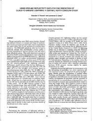
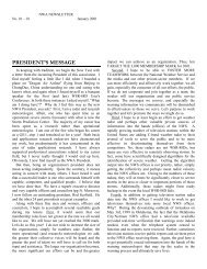
Fig. 1. Rawinsonde measured sounding at Edwards Air Force Base, California, 1800 UTC 30 January 1998. The temperature <strong>and</strong> dew<br />
point temperature profiles are displayed on a st<strong>and</strong>ard Skew-Tliog p diagram. Winds (in knots) are plotted to the right of the display. A hodograph<br />
of the winds is in the upper right. A st<strong>and</strong>ard atmosphere height sC,ale is located to the right of the winds.<br />
the upper limit of RiE in which the probability is greater<br />
than zero, the lower limit of RiE = 0.25 being 100% probability.<br />
Since the mean TKE is quantitative, the higher<br />
the Ri max , the weaker the relation between the probability<br />
of <strong>turbulence</strong> <strong>and</strong> its mean intensity. The mean TKE<br />
may be the integration of a large number of small <strong>turbulence</strong><br />
events or of a small number of large <strong>turbulence</strong><br />
events. The latter is far more important to <strong><strong>air</strong>craft</strong> <strong>turbulence</strong><br />
forecasting than the former. Ideally, the Rimax<br />
should be 0.25 so the probability of <strong>turbulence</strong> with Ri <<br />
0.25 is near 100%.<br />
3. Gravity Wave Modification of Wind Shears <strong>and</strong><br />
Stabilities<br />
The closer one can estimate RiL in (3), the closer one can<br />
set Ri max to 0.25 <strong>and</strong> have greater confidence in (3) as an<br />
<strong><strong>air</strong>craft</strong> <strong>turbulence</strong> forecast tool (McCann 1999). A <strong>gravity</strong><br />
wave is one mechanism that locally modifies RiE. Kondo et<br />
al. (1978) noted that the <strong>turbulence</strong> intermittency at RiE ><br />
0.25 was due to <strong>gravity</strong> <strong>waves</strong>. The theory of how <strong>gravity</strong><br />
<strong>waves</strong> locally increase wind shear <strong>and</strong> reduce stability<br />
have been known for many years (Roach 1970).<br />
Consider the following pilot report received at the<br />
Aviation Weather Center (AWC) on 30 January 1998:<br />
LAX UUA IOV LAX-LAX 050050ITM 18061<br />
FL325ITP B767/SK CLRIWV 290/2500463201<br />
256140 330/260146ITB DURC LAX SMTH 290-<br />
320 MDT SMTH ABVI RM STG SHR 290-320<br />
Heights are given in hundreds of feet above sea level<br />
<strong>and</strong> winds in knots. The <strong>turbulence</strong> group (TB) decodes<br />
as smooth during climb out of Los Angeles, California,<br />
(LAX) except for moderate <strong>turbulence</strong> between 29,000<br />
feet <strong>and</strong> 32,000 feet (8800 m to 9800 m). Winds (WV)<br />
measured by this modern <strong><strong>air</strong>craft</strong>'s (Boeing 767) inertial<br />
navigation system are typically very accurate <strong>and</strong><br />
show a large increase from 250 degrees/46 knots (24 m<br />
sec· I) to 256 degrees/140 knots (72 m sec·1) in the layer<br />
within which the <strong>turbulence</strong> occurred.<br />
Compare the <strong><strong>air</strong>craft</strong>'s observed winds with those<br />
shown in Fig. 1 which are from a rawinsonde observation<br />
launched at Edwards Air Force Base, California, (EDW)<br />
just 40 km to the northwest of the <strong><strong>air</strong>craft</strong>'s location<br />
about the same time as the pilot report. The winds at
J<br />
6<br />
National Weather Digest<br />
200<br />
250<br />
300<br />
350<br />
400<br />
450<br />
500<br />
(<br />
~<br />
y--- V ----- -<br />
/'<br />
/'<br />
f---<br />
~ .......<br />
-~ !.---<br />
o 1 2 3 4 5 6 7 8 9 10<br />
980130/1800VOOO 34.5;-117.6 RUC RICHARDSON NUMBER<br />
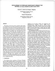
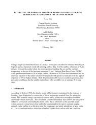
Fig. 2. A vertical profile of the Richardson number between 500 mb <strong>and</strong> 200 mb from the<br />
1800 UTC 30 January 1998, Rapid Update Cycle numerical model at a location approximately<br />
50 nautical miles northeast of Los Angeles, California. This is near the location of the<br />
<strong><strong>air</strong>craft</strong> in the pilot report in the text. The 350-mb level is about 27,000 feet (8200 m) MSL; the<br />
300-mb level is about 30,000 feet (9100 m) MSL; <strong>and</strong> the 250-mb level is about 34,000 feet<br />
(10,400 m) MSL.<br />
29,000 feet are from about 285<br />
degrees/70 knots (36 m sec·I ), not<br />
the 250/46 knots reported by the<br />
<strong><strong>air</strong>craft</strong>. The winds at 32,000 feet<br />
are about 275 degrees/115 knots<br />
(60 m sec·l ) on the rawinsonde <strong>and</strong><br />
256/140 knots from the <strong><strong>air</strong>craft</strong>. The<br />
vertical shear from the <strong><strong>air</strong>craft</strong> is<br />
more than three times that from the<br />
rawinsonde.<br />
Since the difference between<br />
these observations is much greater<br />
than the known errors expected for<br />
either system (Schwartz <strong>and</strong><br />
Benjamin 1995), one must conclude<br />
that each observation recorded a<br />
different wind pattern even though<br />
both were taken in close proximity<br />
of each other. The 1800 UTC Rapid<br />
Update Cycle (RUC) wind analysis<br />
at the location of the <strong><strong>air</strong>craft</strong> shown<br />
in Fig. 2 is similar to the rawinsonde's.<br />
The <strong><strong>air</strong>craft</strong> reported<br />
SMOOTH at the lowest RiE near<br />
the 27,000 foot (8200 m) flight level.<br />
The wind shear measured by the<br />
<strong><strong>air</strong>craft</strong> may have been enhanced by<br />
a <strong>gravity</strong> wave. Using the dispersion<br />
relation for the vertically propagating<br />
component of the wave,<br />
Palmer et al. (1986) <strong>and</strong> Dunkerton<br />
(1997) derived the wave's impact on<br />
the local vertical shear in a non-<br />
I~ ~--------------------------------n<br />
10r--------------------------------,<br />
r:il<br />
g<br />
100<br />
8<br />
NON-TURBULENT<br />
TURBULENT<br />
2<br />
0.1 L-__ -'--__ -'-__ -'-__ ---'-__ ---'-__ ---''--__ -'-----'<br />
0.0 0.5 1.0 1.5 2.0<br />
Non-dimensional amplitude (a)<br />
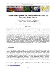
Fig. 3. Curve of the bounding value of the environmental<br />
Richardson number as a function of the non-dimensional amplitude<br />
(a). When (a, RiE) falls in the TURBULENT region, a <strong>gravity</strong><br />
wave will locally increase the wind shear sufficiently to reduce the<br />
local Richardson number to 0.25.<br />
7tl2 1t 31[/2 21t<br />
Gravity Wave Phase Angle<br />
Fig. 4. The ratio of the total local TKE production to the TKE production<br />
by the environmental wind shear as computed for the<br />
30 January 1998 case of the B767 <strong><strong>air</strong>craft</strong> ascent out of Los<br />
Angeles, California, using equation (2) in the text. The wind shear<br />
<strong>and</strong> stability were modified using Eqs. (4) <strong>and</strong> (5) with a = 1.98.<br />
The turbulent Pr<strong>and</strong>tl number, KrnlKh = 0.25.
Volume 25 Numbers 1,2 June 2001<br />
7<br />
rotating environment:<br />
(OV) = (OV)(1 + Ri~2asin¢) (4)<br />
oz L OZ<br />
<strong>and</strong> the wave's impact on the local stability:<br />
The non-dimensional amplitude, a = Nal I V-c I (where a<br />
is the actual amplitude of the wave) is an inverse Froude<br />
number. The denominator is the Doppler-adjusted wind<br />
velocity where c is the phase velocity of the wave<br />
(Dunkerton 1997). When a > 1.0, wave overturning<br />
begins. The nondimensional amplitude will be high when<br />
any of three environmental variables are sufficiently<br />
favorable, 1) high <strong>gravity</strong> wave amplitude, 2) high stability,<br />
<strong>and</strong> 3) low difference between the wind <strong>and</strong> the wave<br />
velocities. When the wind velocity equals the wave velocity,<br />
the wind is said to be at a "critical" value with respect<br />
to the wave (Dunkerton 1997). The <strong>gravity</strong> wave phase<br />
angle,
8<br />
National Weather Digest<br />
Table 1. Unbalanced <strong>flow</strong> diagnostics <strong>and</strong> their sources.<br />
NAME<br />
Inertial Advective Wind<br />
FORMULA<br />
v'nad =<br />
Iv·vvl<br />
I<br />
SOURCE<br />
Uccellini et al. (1984)<br />
Unbalanced Ageostrophic Wind<br />
v',age = ~lvl2 - (V g • v"g r<br />
Koch <strong>and</strong> Dorian (1988)<br />
Divergence Tendency<br />
1400<br />
1200<br />
1000<br />
t.! 800 0<br />
go<br />
~<br />
-~<br />
600<br />
400<br />
1208<br />
Anticyclonic Instability<br />
dD 2<br />
dt = -V ct> + 2J(u, v)+ Is - fJ u<br />
(r; + 1)(Scurv + ~) < °<br />
Zack <strong>and</strong> Kaplan (1987)<br />
Alaka (1961)<br />
ance of weak forces in these cases is small which should<br />
lead to weak <strong>gravity</strong> wave production.<br />
Koch <strong>and</strong> Dorian (1988) introduced the second <strong>unbalanced</strong><br />
<strong>flow</strong> indicator in the Table 1 list. Their study connected<br />
the source of a mesoscale <strong>gravity</strong> wave event with<br />
a region of <strong>unbalanced</strong> <strong>flow</strong>. The indicator they chose to<br />
compute was an <strong>unbalanced</strong> ageostrophic Rossby number<br />
which is the ratio of the component ofthe ageostrophic<br />
wind normal to the <strong>flow</strong> to the wind speed itself For the<br />
same reason as above, the <strong>unbalanced</strong> ageostrophic wind<br />
in Table 1 is their Rossby number multiplied by the wind<br />
speed.<br />
The third <strong>unbalanced</strong> <strong>flow</strong> indicator has a long history.<br />
It is derived from taking the horizontal divergence of<br />
the equation of horizontal motion. When dD/dt = 0, the<br />
equation is sometimes known as the nonlinear balance<br />
equation. Charney (1955) noted that when the divergence<br />
tendency is zero everywhere, the wind <strong>and</strong> the mass<br />
fields are in balance, <strong>and</strong> the integration of primitive<br />
equations in early numerical models could proceed without<br />
getting unwanted <strong>gravity</strong> <strong>waves</strong>. Uccellini <strong>and</strong> Koch<br />
(1987) <strong>and</strong> Zack <strong>and</strong> Kaplan (1987) showed how significant<br />
divergence growth leads to <strong>unbalanced</strong> <strong>flow</strong>.<br />
Knox (1997 a) discussed sources of <strong>unbalanced</strong> <strong>flow</strong> in<br />
anticyclonic <strong>flow</strong>, that is inertial instability <strong>and</strong> gradient<br />
<strong>flow</strong> non-ellipticity. The former is the familiar instability<br />
of negative absolute vorticity (in the Northern<br />
Hemisphere). The latter occurs when winds are "anomalous,"<br />
or high enough to produce imaginary solutions to<br />
the quadratic gradient wind equation. Alaka (1961)<br />
derived a general anticyclonic instability criterion on an<br />
isentropic surface that is the product of these two "instabilities."<br />
The listing in Table 1 is somewhat of a simplification<br />
of that criterion in that the curvature vorticity is<br />
computed on "level" pressure surfaces <strong>and</strong> with stream-<br />
200<br />
0<br />
LlGlIT· MODERAlE MODERAlE· SEVERE<br />
MODERAlE<br />
SEVERE<br />
Turbulence Intensity<br />
Fig. 5. The distribution of the AWe database pilot report <strong>turbulence</strong><br />
greater than a particular intensity.<br />
line curvatures instead of trajectory curvatures. In most<br />
cases, these simplifications will overestimate the negative<br />
curvature vorticity. AB the subsequent results will<br />
show, these simplifications do not seem to hurt this index<br />
as an <strong>unbalanced</strong> <strong>flow</strong>/<strong>turbulence</strong> indicator.<br />
5. Observations of Unbalanced Flow Indicators <strong>and</strong><br />
Turbulence<br />
Environmental Richardson numbers, wind shears, <strong>and</strong><br />
the above <strong>unbalanced</strong> <strong>flow</strong> diagnostics were computed for<br />
each of 1832 pilot reports above the 20,000 foot (6100 m)<br />
flight level in a database gathered every workday from<br />
1 October 1996 to 31 January 1997. TheAWC receives hundreds<br />
of <strong>turbulence</strong> pilot reports each day. Pilot reports are<br />
notorious for low quality <strong>and</strong> cannot be automatically<br />
processed with sufficient quality control (Schwartz 1996).<br />
In order to manage this large volume <strong>and</strong> to ensure that the<br />
reports were of high quality, the pilot reports were manually<br />
sampled. Every three hours (0000 UTC, 0300 UTC, etc.)<br />
available reports over the contiguous United States plus or<br />
minus one hour of the observation time were added to the<br />
database in this manner: all reports SEVERE or MODER<br />
ATE-SEVERE, one MODERATE or LIGHT-MODERATE,<br />
one LIGll, <strong>and</strong> one SMOOTH. Ifmore than ten MODER<br />
ATE reports occurred in the period, then one additional<br />
report was added. Reports MODERATE or less were chosen<br />
r<strong>and</strong>omly. Care was taken to make certain of a pilot<br />
report's details <strong>and</strong> to exclude reports in known thunderstorms<br />
or mountain <strong>waves</strong>. Included are reports of "chop,"<br />
which, in a pure sense, is not <strong>turbulence</strong> but is often mistakenly<br />
reported in turbulent conditions. The goal was to<br />
sample the environmental conditions of all <strong>turbulence</strong><br />
intensities in order to discern their differences. The database<br />
is not a statistical sample of all <strong>turbulence</strong> pilot
Volume 25 Numbers 1, 2 June 2001<br />
9<br />
Table 2. Postagreement Richardson number <strong>and</strong> wind shear<br />
squared (foundations of traditional CAT diagnostics) <strong>and</strong> of various<br />
<strong>unbalanced</strong> <strong>flow</strong> diagnostics with MODERATE or greater <strong>turbulence</strong><br />
pilot reports. The statistics are based on 1832 "r<strong>and</strong>omly"<br />
selected pilot reports of <strong>turbulence</strong> above 20,000 foot (6100<br />
m) flight level between I October 1996 <strong>and</strong> 31 January 1997. The<br />
number to the right of each slash is the number of times the value<br />
of the <strong>unbalanced</strong> <strong>flow</strong> diagnostic exceeded the threshold. The<br />
number to the left of the slash is the number of those pilot reports<br />
exceeding the threshold with <strong>turbulence</strong> intensities MODERATE<br />
or greater.<br />
15 77/90 = .86<br />
> 20<br />
> 25<br />
35/43 = .82<br />
12/14 = .86<br />
>30 5/5=1 .00<br />
Anticyclonic Instability (AI)<br />
< 0 (x10' to ) sec"<br />
< -5<br />
< -10<br />
10<br />
National Weather Digest<br />
980130/1BOOVOOO 300 HB ISOTACHS (knots)<br />
9B0130/1800VOOO 300 HB STREAMLINES<br />
300 HB STRAIGHT FLOH INERTIAL ADVECTIVE<br />
980130/1800VOOO 300 HB STREAMLINES
Volume 25 Numbers 1,2 June 2001 11<br />
200 ..--<br />
250<br />
300<br />
350<br />
400<br />
450<br />
(<br />
/V /<br />
'\<br />
~ _. __.<br />
~<br />
V :/<br />
/'<br />
I><br />
-<br />
UL<br />
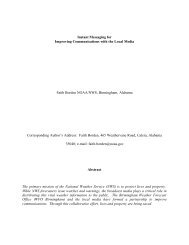
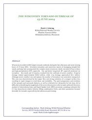
Fig. 6. a) RUC 300-mb streamlines<br />
<strong>and</strong> isotachs for 1800 UTC<br />
30 January 1998 over southern<br />
California. b) RUC 300-mb<br />
streamlines <strong>and</strong> inertial advective<br />
wind. (See Table 1 for definition.)<br />
c) Same as Fig. 2 except<br />
a profile of the inertial advective<br />
wind. d) Same as Fig. 2 except<br />
a profile of the divergence tendency.<br />
The dark circle in a) <strong>and</strong><br />
b) locates the <strong><strong>air</strong>craft</strong> position at<br />
1806 UTC 30 January 1998.<br />
500 - -<br />
-10<br />
o 10 20 30 40 50 60 70 80 90<br />
980130/1800VOOO 34.5;-117.6 RUC INERTIAL ADVECTIVE WIND (knt)<br />
200<br />
250<br />
\<br />
1\<br />
300<br />
350<br />
400<br />
450<br />
/<br />
V<br />
/<br />
500<br />
-50<br />
-40 -30 -20 -10 o 10 20 30 40 50<br />
980130/1800VOOO 34.5;-117.6 RUC DIVERGENCE TENDENCY (*10**-9 /sec**2)
12<br />
National Weather Digest<br />
What about the pilot report in Section 3? Figure 6<br />
shows selected synoptic aspects of this case. The vertical<br />
profile of the inertial advective wind in Fig. 6c showed<br />
that it exceeded 50 knots (26 m S·l) from about 29,000 ft<br />
to 32,000 ft, precisely the layer in which the <strong><strong>air</strong>craft</strong> experienced<br />
the <strong>turbulence</strong>. The vertical profile of divergence<br />
tendency in Fig. 6d showed the highest values in this<br />
layer <strong>and</strong> slightly below this layer but the absolute values<br />
were low compared with Table 3 values. The <strong>flow</strong> in<br />
all layers was not anticyclonic enough to be unstable<br />
according to the formula for anticyclonic instability.<br />
Gravity <strong>waves</strong> from other sources were unlikely since<br />
there was no convection in the area <strong>and</strong> the <strong>flow</strong> profile<br />
was not favorable with the underlying terrain for mountain<br />
<strong>waves</strong>. Therefore, given all the data from this case,<br />
the <strong>turbulence</strong> event was probably caused by a <strong>gravity</strong><br />
wave which probably resulted from <strong>unbalanced</strong> <strong>flow</strong>.<br />
5. Conclusions<br />
There is ample theory showing that <strong>gravity</strong> <strong>waves</strong> can<br />
cause <strong>turbulence</strong> through the modification of the environmental<br />
Richardson number to a local Richardson<br />
number less than the critical Richardson number for <strong>turbulence</strong>.<br />
The theory allows for a Pr<strong>and</strong>tl number in the<br />
TKE equation to approach or equal the critical<br />
Richardson number, thereby reducing the uncertainty of<br />
<strong>turbulence</strong> occurrence. The theory supports observations<br />
by Beckman (1981) <strong>and</strong> others who have connected wave<br />
clouds on satellite images with CAT reports.<br />
The respective theoretical roles of environmental wind<br />
shear, Richardson number, <strong>and</strong> <strong>unbalanced</strong> <strong>flow</strong> suggest<br />
an ingredients-based CAT forecast technique similar to<br />
thunderstorm forecasting (Doswell et aI, 1996).<br />
Environmental layers favorably setup with high wind<br />
shear <strong>and</strong> low Richardson number should be given first<br />
consideration. In these layers only minimal <strong>gravity</strong> wave<br />
forcing is necessary to trigger CAT. Regions of highly<br />
<strong>unbalanced</strong> <strong>flow</strong> may produce high amplitude <strong>gravity</strong><br />
<strong>waves</strong> sufficient by themselves to produce CAT.<br />
The governing TKE equations to quantifY this technique<br />
are (2) combined with (4) <strong>and</strong> (5) or (3) combined<br />
with (6). The problem is to find the non-dimensional<br />
amplitudes (a) of <strong>unbalanced</strong> <strong>flow</strong> <strong>waves</strong>. Knowing a, one<br />
can compute the maximum TKE production from the<br />
local modifications to the wind shear <strong>and</strong> stability.<br />
Section 3 defined a in terms of two environmental variables,<br />
stability <strong>and</strong> wind speed, <strong>and</strong> two wave variables,<br />
the actual wave amplitude <strong>and</strong> the wave phase velocity.<br />
Theoretically <strong>and</strong> observationally, two questions<br />
remain. 1) What are the amplitudes <strong>and</strong> phase velocities<br />
of <strong>unbalanced</strong> <strong>flow</strong> <strong>waves</strong>? In the case of the B767 ascent<br />
out of Los Angeles, there was <strong>unbalanced</strong> <strong>flow</strong> diagnosed,<br />
<strong>and</strong> the <strong><strong>air</strong>craft</strong> winds reported were sufficient to estimate<br />
a. This was a rare pilot report. A successful <strong>turbulence</strong><br />
diagnostic for everyday use by AWC forecasters will<br />
have to make good estimates of a.<br />
2) What are the best diagnostics for <strong>unbalanced</strong> <strong>flow</strong>?<br />
The <strong>unbalanced</strong> <strong>flow</strong> diagnostics presented in Section 3<br />
are not statistically correlated with each other in the<br />
AWC <strong>turbulence</strong> pilot report database, implying more<br />
than one process can cause <strong>unbalanced</strong> <strong>flow</strong>. Ongoing<br />
research at the AWC is aimed at developing better diagnostics.<br />
illtimately, since the horizontal forces on <strong>air</strong><br />
parcels in these cases are <strong>unbalanced</strong> by definition, there<br />
may very well be a single universal diagnostic that will<br />
work well.<br />
While this paper emphasized <strong>unbalanced</strong> <strong>flow</strong> as a<br />
cause of <strong>gravity</strong> <strong>waves</strong>, it is not the only one. Because of<br />
numerous other causes, the analysis of <strong>gravity</strong> wave<br />
sources in an operational environment is going to be very<br />
complex. Furthermore, wave-mean <strong>flow</strong> <strong>and</strong> wave-wave<br />
interactio.ns (Franke <strong>and</strong> Robinson 1999) add more levels<br />
of complexity.<br />
Finally, although it appears that <strong>gravity</strong> <strong>waves</strong> are significant<br />
triggers of CAT, it is much too premature to conclude<br />
that they are an exclusive cause of CAT. There may<br />
be other mechanisms that locally modifY wind shears <strong>and</strong><br />
stabilities so that CAT may form.<br />
Acknowledgments<br />
Many thanks go to John Knox whose feedback on this<br />
paper <strong>and</strong> my work in general has been the basis for any<br />
success I can claim. Roy Darrah <strong>and</strong> Robert Sharman<br />
also gave me valuable reviews.<br />
References<br />
Alaka, M.A., 1961: The occurrence of anomalous winds<br />
<strong>and</strong> their significance. Mon. Wea. Rev., 89, 482-494.<br />
Beckman, S.K, 1981: Wave clouds <strong>and</strong> severe <strong>turbulence</strong>.<br />
Natl. Wea. Dig., 6:3, 30-37.<br />
Blumen, w., 1972: Geostrophic adjustment. Rev. Geophys.<br />
Space Phys., 10,485-528.<br />
Browning, KA., T.w. Harrold, <strong>and</strong> J.R Starr, 1970:<br />
Richardson number limited shear zones in the free<br />
atmosphere. Quart. J. Roy. Met. Soc., 96,40-49.<br />
Cahn,A., 1945: An investigation of the free oscillations of<br />
a simple current system. J. Meteor., 2,113-119.<br />
Charney, J., 1955: The use of the primitive equations of<br />
motion in numerical prediction. Tellus, 7, 22-26.<br />
Cundy, RG., 1999: Use of numerical guidance aids in<br />
forecasting a <strong>turbulence</strong> superoutbreak over the eastern<br />
United States. Proc. Eighth Conf on Aviation, Range, <strong>and</strong><br />
Aerospace Meteorology, Dallas TX, Amer. Meteor. Soc.,<br />
382-386.<br />
Doswell, C.A. III, H.E. Brooks, <strong>and</strong> RA. Maddox, 1996:<br />
Flash flood forecasting: An ingredients based methodology.<br />
Wea. Forecasting, 11,560-581.<br />
Duffy, D.G., 1990: Geostrophic adjustment in a baroclinic<br />
atmosphere. J. Atmos. Sci., 47, 457-473.<br />
Dunkerton, T.J., 1997: Shear instability of inertia-<strong>gravity</strong><br />
<strong>waves</strong>. J. Atmos. Sci., 54, 1628-1641.
Volume 25 Numbers 1,2 June 2001<br />
13<br />
Dutton, JA, <strong>and</strong> HA Panofsky, 1970: Clear <strong>air</strong> <strong>turbulence</strong>:<br />
A mystery may be unfolding. Science, 167,937-944.<br />
Dutton, M.J.O., 1980: Probability forecasts of <strong>clear</strong>-<strong>air</strong><br />
<strong>turbulence</strong> based on numerical model output.<br />
Meteorological Magazine, 109,293-309.<br />
Ellrod, G.P., <strong>and</strong> D.I. Knapp, 1992: An objective <strong>clear</strong>-<strong>air</strong><br />
<strong>turbulence</strong> forecasting technique: Verification <strong>and</strong> operational<br />
use. Wea. Forecasting, 7,150-165.<br />
Franke, P.M. <strong>and</strong> WA Robinson, 1999: Nonlinear behavior<br />
in the propagation of atmospheric <strong>gravity</strong> <strong>waves</strong>. J<br />
Atmos. Sci., 56, 3010-3027.<br />
Fritts, D.C., <strong>and</strong> Z. Luo, 1992: Gravity wave excitation by<br />
geostrophic adjustment of the jet stream. Part 1: Twodimensional<br />
forcing. J Atmos. Sci., 49, 681-697.<br />
Garratt, J.R, 1992: The Atmospheric Boundary Layer.<br />
Cambridge University Press, 316 pp.<br />
Kaplan, M.L., S.E. Koch, Y.L. Lin, RP. Weglarz, <strong>and</strong> RA<br />
Rozumalski, 1997: Numerical simulations of a <strong>gravity</strong><br />
wave event over CCOPE. Part 1: The role of geostrophic<br />
adjustment in mesoscale jetlet formation. Mon. Wea. Rev.,<br />
125,1185-1211.<br />
Kennedy, P.J., <strong>and</strong> MA Shapiro, 1980: Further encounters<br />
with <strong>clear</strong> <strong>air</strong> <strong>turbulence</strong> in research <strong><strong>air</strong>craft</strong>. J<br />
Atmos. Sci., 37, 986-993.<br />
Knox, JA, 1997a: Generalized nonlinear balance criteria<br />
<strong>and</strong> inertial stability. J Atmos. Sci., 54, 967-985.<br />
____ , 1997b: Possible mechanisms of <strong>clear</strong>-<strong>air</strong> <strong>turbulence</strong><br />
in strongly anticyclonic <strong>flow</strong>s. Mon. Wea. Rev.,<br />
125, 1251-1259.<br />
Koch, S.E., <strong>and</strong> P.B. Dorian, 1988: A mesoscale <strong>gravity</strong><br />
wave event observed during CCOPE. Part III: Wave environment<br />
<strong>and</strong> probable source mechanism. Mon. Wea.<br />
Rev., 116, 2570-2592.<br />
Kondo, J., O. Kanechika, <strong>and</strong> N. Yasuda, 1978: Heat <strong>and</strong><br />
momentum transfers under strong stability in the atmospheric<br />
surface layer. J Atmos. Sci., 35,1012-1021.<br />
Lester, P.F. <strong>and</strong> WA Fingerhut, 1974: Lower turbulent<br />
zones associated with mountain lee <strong>waves</strong>. J Appl.<br />
Meteor., 13,54-61.<br />
MacCready, P.B., 1964: St<strong>and</strong>ardization of gustiness values<br />
from <strong><strong>air</strong>craft</strong>, J Appl. Meteor., 3, 439-449 .<br />
McCann, D.W, 1999: A simple turbulent kinetic energy<br />
equation <strong>and</strong> <strong><strong>air</strong>craft</strong> boundary layer <strong>turbulence</strong>. Natl.<br />
Wea. Dig., 23:1-2,13-19.<br />
Mellor, G.L., <strong>and</strong> T. Yamada, 1982: Development of a turbulent<br />
closure model for geophysical fluid problems. Rev.<br />
Geophys. Space Phys., 20, 851-875.<br />
Miles, J. W, <strong>and</strong> L.N. Howard, 1964: Note on a heterogeneous<br />
<strong>flow</strong>. J Fluid Mech., 20, 331-336.<br />
Murphy, EA, RB. D'Agostino, <strong>and</strong> J.P. Noonan, 1982:<br />
Patterns in the occurrences of Richardson numbers less<br />
than unity in the lower atmosphere. J Appl. Meteor., 21,<br />
321-333.<br />
O'Sullivan, D. <strong>and</strong> T.J. Dunkerton, 1995: Generation of<br />
inertia-<strong>gravity</strong> <strong>waves</strong> in a simulated life cycle ofbaroclinic<br />
instability. J Atmos. Sci., 52, 3695-3716.<br />
Palmer, T.N., G.J. Shutts, <strong>and</strong> R Swinbank, 1986:<br />
Alleviation of a systematic westerly bias in general circulation<br />
<strong>and</strong> numerical weather prediction models through<br />
an orographic <strong>gravity</strong> wave drag parameterization.<br />
Quart. J Roy. Met. Soc., 112, 1001-1039.<br />
Reed, RJ. <strong>and</strong> KR Hardy, 1972: A case study of persistent,<br />
intense, <strong>clear</strong> <strong>air</strong> <strong>turbulence</strong> in an upper level<br />
frontal zone. J Appl. Meteor., 11, 541-549.<br />
Roach, WT., 1970: On the influence of synoptic development<br />
on the production of high level <strong>turbulence</strong>. Quart. J<br />
Roy. Met. Soc., 96, 413-429.<br />
Rockey, c., <strong>and</strong> D.W McCann, 1995: Turbulent kinetic<br />
energy production in significant <strong>turbulence</strong> events. Proc.<br />
Sixth Conf on Aviation Weather Systems, Dallas TX,<br />
Amer. Meteor. Soc., 166-169.<br />
Rossby, C.G., 1938: On the mutual adjustment of pressure<br />
<strong>and</strong> velocity distributions in simple current systems, Part<br />
II. J Mar. Res., 1,239-263.<br />
Schwartz, B., 1996: The quantitative use of PIREPs in<br />
developing aviation weather guidance products. Wea.<br />
Forecasting, 11, 372-384.<br />
____ , <strong>and</strong> S.G. Benjamin, 1995: A comparison of<br />
temperature <strong>and</strong> wind measurements from ACARSequipped<br />
<strong><strong>air</strong>craft</strong> <strong>and</strong> rawinsondes. Wea. Forecasting, 10,<br />
528-544.<br />
Thorpe, SA, 1969: Experiments on the stability of stratified<br />
shear <strong>flow</strong>s. Radio Sci., 4,1327-1331.<br />
Uccellini, L.W, P.J. Kocin, RA Petersen, C.H. Wash, <strong>and</strong><br />
KF. Brill, 1984: The President's Day cyclone of 18-19<br />
February 1979: Synoptic overview <strong>and</strong> analysis of the<br />
subtropical jet streak influencing the pre-cyclogenetic<br />
period. Mon. Wea. Rev., 112,31-55.<br />
____:, <strong>and</strong> S.E. Koch, 1987: The synoptic setting <strong>and</strong><br />
possible energy sources for mesoscale wave disturbances.<br />
Mon. Wea. Rev., 115, 721-729.<br />
van Tuyl, AH., <strong>and</strong> JA Young, 1982: Numerical simulation<br />
of nonlinear jet streak adjustment. Mon. Wea. Rev.,<br />
110,2038-2054.
14<br />
National Weather Digest<br />
Vinnichenko, N.K., N.Z. Pinus, S.M. Shmeter, <strong>and</strong> G.N.<br />
Shur, 1980: Turbulence in the Free Atmosphere,<br />
Consultants Bureau, 310 pp.<br />
Weglarz, RP., <strong>and</strong> Y-L Lin, 1997: A linear theory for jet<br />
streak formation due to zonal momentum forcing in a<br />
stably stratified atmosphere. J. Atmos. Sci., 54, 908-932.<br />
Zack, J.W, <strong>and</strong> M.L. Kaplan, 1987: Numerical simulations<br />
of the subsynoptic features associated with the<br />
AVE-SESAME I case. Part 1. The preconvective environment.<br />
Mon. Wea. Rev., 115,2367-2394.<br />
a<br />
a<br />
c<br />
o<br />
f<br />
Appendix<br />
List of Symbols<br />
<strong>gravity</strong> wave amplitude<br />
non-dimensional <strong>gravity</strong> wave amplitude<br />
<strong>gravity</strong> wave phase velocity<br />
horizontal divergence of the wind<br />
Coriolis parameter<br />
9 acceleration due to <strong>gravity</strong><br />
J<br />
Kh<br />
Km<br />
N<br />
Jacobian operator<br />
eddy thermal diffusivity<br />
eddy viscosity<br />
stability<br />
Pr Pr<strong>and</strong>tl number (Krr/ K h )<br />
Ri<br />
Ro<br />
Richardson number<br />
Rossby number<br />
time<br />
u<br />
V<br />
v<br />
Vag<br />
Vg<br />
Vinad<br />
Vuage<br />
z<br />
x-component of the wind<br />
mean horizontal wind<br />
y-component of the wind<br />
ageostrophic wind<br />
geostrophic wind<br />
inertial advective wind<br />
<strong>unbalanced</strong> ageostrophic wind<br />
vertical coordinate<br />
13 change in Coriolis parameter with latitude<br />
E<br />
rate of turbulent kinetic energy dissipation<br />