A Program for Calculating the Montgomery Stream Function

Volume 20 Number 3 March, 1996
55
(4) Determine T from the average of To and Tb
T = Tb + To
2
(19)
(5) Substitute results from steps (1)-(4) into (17) to find M.
These steps can be translated into common computer languages,
or encoded as a macro in upper-air and gridded-data
processing packages which allow the user to find the nearest
isobaric sUlfaces above and below an isentropic suiface of
interest. A simple FORTRAN program which computes M is
shown in the Appendix. If the comments are removed, the
program is very short and easily typed with a text editor or
word processor. The program assumes that the user has information
from isobaric surfaces above and below the isentropic
surface of interest. In practice this information would likely be
contained in arrays so that the user would reference array elements
instead of READ statements (or other language-specific
input statements). Input isobaric data and M for two analyses
along the 319.5 K isentropic surface are given in Tables 1
and 2 in the Appendix. The data are taken from 3-h CLASS
radiosonde observations at 2100 UTC 8 March 1992 - 0000
UTC 9 March 1992 during STORM-FEST (STormscale Operational
and Research Meteorology-Fronts Experiment Systems
Test) (Cunning and Williams 1993). As part of STORM-FEST,
flow along the 319.5 K isentropic surface was followed by
an instrumented aircraft (Prater 1994) during lee cyclogenesis
(Mahoney et al. 1995).
3. Results
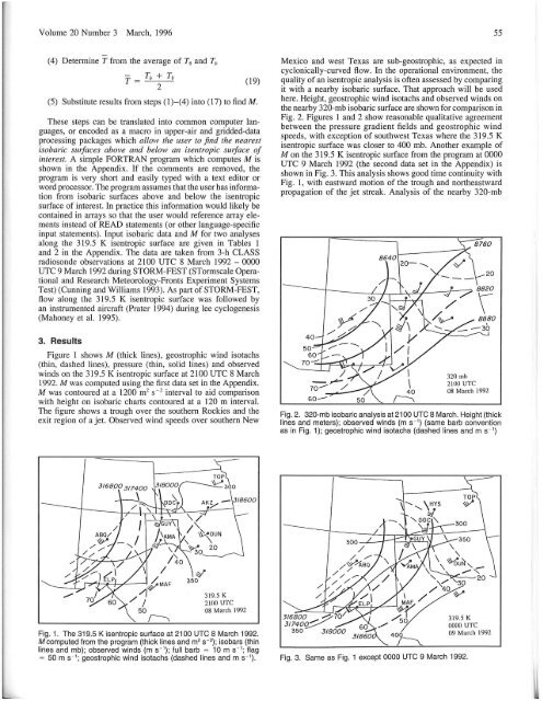
Figure 1 shows M (thick lines), geostrophic wind isotachs
(thin, dashed lines), pressure (thin, solid lines) and observed
winds on the 319.5 K isentropic surface at 2100 UTC 8 March
1992. M was computed using the first data set in the Appendix.
M was contoured at a 1200 m 2 S - 2 interval to aid comparison
with height on isobaric charts contoured at a 120 m interval.
The figure shows a trough over the southern Rockies and the
exit region of a jet. Observed wind speeds over southern New
Mexico and west Texas are sub-geostrophic, as expected in
cyclonically-curved flow. In the operational environment, the
quality of an isentropic analysis is often assessed by comparing
it with a nearby isobaric surface. That approach will be used
here. Height, geostrophic wind isotachs and observed winds on
the nearby 320-mb isobaric surface are shown for comparison in
Fig. 2. Figures 1 and 2 show reasonable qualitative agreement
between the pressure gradient fields and geostrophic wind
speeds, with exception of southwest Texas where the 319.5 K
isentropic surface was closer to 400 mb. Another example of
M on the 319.5 K isentropic surface from the program at 0000
UTC 9 March 1992 (the second data set in the Appendix) is
shown in Fig. 3. This analysis shows good time continuity with
Fig. 1, with eastward motion of the trough and northeastward
propagation of the jet streak. Analysis of the nearby 320-mb
8640 20----.
320 mh
2100 UTe
08 March 1992
Fig. 2. 320-mb isobaric analysis at 21 00 UTe 8 March . Height (thick
lines and meters); observed winds (m s- ') (same barb convention
as in Fig. 1); geostrophic wind isotachs (dashed lines and m s- ')
319.5 K
2100 UTe
08 March 1992
Fig. 1. The 319.5 K isentropic surface at 2100 UTe 8 March 1992.
M computed from the program (thick lines and m 2 s -2); isobars (thin
lines and mb); observed winds (m s- '); full barb = 10 m s- '; flag
= 50 m s-'; geostrophic wind isotachs (dashed lines and m s- ').
'-..40~
319.5 K
0000 UTe
09 March 1992
Fig. 3. Same as Fig. 1 except 0000 UTe 9 March 1992.