Identification of Grape Varieties via Digital Leaf Image ... - Oiv2010.ge

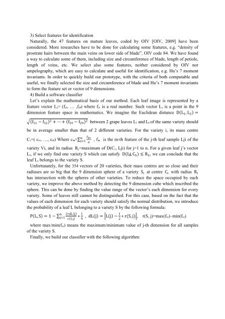
3) Select features for identification
Naturally, the 47 features on mature leaves, coded by OIV [OIV, 2009] have been
considered. More researches have to be done for calculating some features, e.g. “density of
prostrate hairs between the main veins on lower side of blade”, OIV code 84. We have found
a way to calculate some of them, including size and circumference of blade, length of petiole,
length of veins, etc. We select also some features, neither considered by OIV nor
ampelography, which are easy to calculate and useful for identification, e.g. Hu‟s 7 moment
invariants. In order to quickly build our prototype, with the criteria of both computable and
useful, we finally selected the size and circumference of blade and Hu‟s 7 moment invariants
to form the feature set or vector of 9 dimensions.
4) Build a software classifier
Let‟s explain the mathematical basis of our method. Each leaf image is represented by a
feature vector Lj= (fj1, … ,fj9) where fji is a real number. Such vector Lj is a point in the 9
dimension feature space in mathematics. We imagine the Euclidean distance D L 1 , L 2 =
f 11 − f 12 2 + ⋯ + f 19 − f 29 2 between 2 grape leaves L1 and L2 of the same variety should
be in average smaller than that of 2 different varieties. For the variety i, its mass centre
Ci=( ci1, …, ci9) Where cim=
n
f jm
j=1 , fjm is the m-th feature of the j-th leaf sample Lji of the
n
variety Vi, and its radius R i =maximum of D(Ci, Lji) for j=1 to n. For a given leaf j‟s vector
Lj, if we only find one variety S which can satisfy D(Lj, C S ) ≤ R S , we can conclude that the
leaf Lj belongs to the variety S.
Unfortunately, for the 354 vectors of 20 varieties, their mass centres are so close and their
radiuses are so big that the 9 dimension sphere of a variety S i at centre C i with radius R i
has intersection with the spheres of other varieties. To reduce the space occupied by each
variety, we improve the above method by detecting the 9 dimension cube which inscribed the
sphere. This can be done by finding the value range of the vector‟s each dimension for every
variety. Some of leaves still cannot be distinguished. For this case, based on the fact that the
values of each dimension for each variety should satisfy the normal distribution, we introduce
the probability of a leaf L belonging to a variety S by the following formula:
P L, S = 1 −
9 2∗dL j
j=1 ∗ 1 , dL j = L j − 1 r S,j 9 2
∗ r(S, j) , r(S, j)=max(fsj)–min(fsj)
where max/min(fsj) means the maximum/minimum value of j-th dimension for all samples
of the variety S.
Finally, we build our classifier with the following algorithm: