A Method for Gradient Enhancement of Continuum Damage Models

TECHNISCHE MECHANIK, Band 28, Heft 1, (2008), 43 – 52
Manuskripteingang: 31. August 2007
A Method for Gradient Enhancement of Continuum Damage Models
B. J. Dimitrijevic, K. Hackl
A method for the regularization of continuum damage material models based on gradient-type enhancement of the
free-energy functional is presented. Direct introduction of the gradient of the damage variable would require C 1
interpolation of the displacements, which is a complicated task to achieve with quadrilateral elements. Therefore
a new variable field is introduced, which makes the model non-local in nature, while preserving C 0 interpolation
order of the variables at the same time. The strategy is formulated as a pure minimization problem, therefore
the LBB-condition does not apply in this case. However, we still take the interpolation of the displacement field
one order higher than the interpolation of the field of additional (non-local) variables. That leads to increased
accuracy and removes the post-processing step necessary to obtain consistent results in the case of equal interpolation
order. Several numerical examples which show the performance of the proposed gradient enhancement
are presented. The pathological mesh dependence of the damage model is efficiently removed, together with the
difficulties of numerical calculations in the softening range. Calculations predict a development of the damage
variable which is mesh-objective for fixed internal material length.
1 Introduction
When utilizing conventional inelastic material models with softening effects, the presence of softening leads to
ill-posed boundary value problems due to the loss of ellipticity of the governing field equations. Ill-posedness
manifests itself by the fact that the resulting algebraic system has no unique solution or by a strong mesh dependence
of the obtained results. For softening material behavior the deformation tends to localize in a narrow band,
the band width only restricted by the mesh resolution. To overcome this problem there are several strategies proposed
that take into consideration an internal material length scale. The most effective ones introduce non-local
terms in the model. That task can be accomplished following two approaches: integral-type and gradient-type.
The integral strategy introduces non-local variables as weighted averages of the local internal variables of the
points near the point under consideration, see Bažant and Jirásek (2002). The application of nonlocal integral
models together with inelastic materials is not very efficient from the computational point of view, since a global
averaging procedure is required and consequently the resulting equations cannot be linearized easily.
The gradient strategy introduces higher order gradient terms (mostly Laplacian) of the non-local variable into the
differential equation governing the evolution of control variables. There are several choices for the variable to
be represented non-localy. In the works of Peerlings et al. (1998), (Peerlings, 1999), Simone et al. (2003) this is
the equivalent strain measure, whose non-local counterpart is used in the calculation of the damage value. The
corresponding differential equation involving the Laplacian of the non-local variable is further integrated using
a generalized principle of virtual work. An alternative approach can be found in works by Nedjar (2001) and
Makowski et al. (2006). The Laplacian term is there directly introduced into the differential equation governing
the damage evolution, and the governing system of equations is then integrated using a generalized principle of
virtual power. There is also an approach, similar to the one used in the present paper, presented in the work of
Peerlings et al. (2004). The variable to be represented non-locally is the equivalent strain measure and the gradient
enhancement is achieved by introduction of additional terms in the free energy functional (norm of the non-local
variable’s gradient and the penalized difference between the equivalent strain and its non-local counterpart). Such
approach leads, however, to the evolution of non-locality even in the purely elastic case.
In the present contribution a method is presented that is based on the enhancement of free energy function using the
gradients of the damage variable, as in (Dimitrijevic and Hackl, 2006). Direct introduction of the gradient of the
inelastic variables would require C 1 interpolation of the displacements, which is a complicated task to achieve with
quadrilateral elements, see i.e. de Borst and Pamin (1996). Therefore is a new variable introduced, which serves
43

to transport the values of the inelastic variables across the element boundaries. That makes the model non-local
in nature, while preserving C 0 interpolation order of the variables at the same time, see (Peerlings, 1999). The
price to pay is an additional set of equations which has to be satisfied on the structural level, involving non-local
variables and their derivatives.
The paper is organized as follows. Section 2 introduces the enhancement in the form of a pure minimization
problem and presents the resulting global system of equations. Section 3 explains the constitutive model and
Section 4 focuses on the finite element implementation. In Section 5 we show some representative simulation
results. Conclusions are finally gathered in Section 6.
2 Gradient Enhancement of a Continuum Damage Model
In order to perform the gradient enhancement, the starting point is a free energy function commonly used in
continuum modeling of isotropic scalar damage:
ψ = 1 f(d) (ɛ : C : ɛ) (1)
2
In (1) d represents a scalar variable that measures the degree of the material stiffness loss, and f(d) some appropriate
function that is at least twice differentiable and satisfies the conditions:
f(d) : R + → (0, 1] |
{
f(0) = 1,
}
lim f(d) = 0
d→∞
These conditions assure pure elastic behavior of the undamaged material and the complete material stiffness loss in
the limiting case d → ∞. The guiding idea was to enhance the free energy function introducing a term involving
the squared norm of the damage parameter gradient:
¯ψ = 1 2 f(d) (ɛ : C : ɛ) + c d
2 ‖∇d‖2 (3)
Direct utilization of the form (3) poses a very strong requirement on the displacement interpolation field: it is
required that the displacement becomes C 1 continuous. An alternative simplified, but still relatively complicated
approach can be to follow the super-element strategy of Abu Al-Rub and Voyiadjis (2005). In the present work,
the modification of the enhanced free energy function is performed introducing an additional variable field ϕ, as
in (Dimitrijevic and Hackl, 2006), that should transfer the values of the damage parameter across the element
boundaries thus making it non-local in nature. Besides the gradient term in the non-local variable ϕ, the modified
free energy function includes a term which penalizes the difference between the non-local and local field:
˜ψ = 1 2 f(d) (ɛ : C : ɛ) + c d
2 ‖∇ϕ‖2 + β d
2 [ϕ − γ 1d] 2 (4)
In (4) parameter β d represents the energy penalizing the difference between non-local and local field, c d represents
the gradient parameter that defines the degree of gradient regularization and the internal length scale. Finally a
parameter γ 1 is used as a switch between the local and enhanced model: setting γ 1 = 0 and c d = 0 one obtains
a local model, while setting γ 1 = 1 and c d ≠ 0 leads to the regularized model. Its introduction is motivated
entirely by numerical reasons, so that we are able to obtain a non-singular tangent matrix in the limiting local case.
Having the enhanced free energy function defined, the potential functional can be written in a standard manner:
Π =
∫
Ω
∫
˜ψ dV − u · (ρb) dV −
Ω
∫
∂Ω σ
u · t dA (5)
In (5) ρb stands for the force per unit volume of the body Ω and t for the external loading per unit surface of the
boundary of the body ∂Ω σ . Minimization of the potential (5) with respect to the primal variables u and ϕ results
in a system of equations that has to be solved globally:
∫
Ω
δɛ : ∂ ˜ψ
∂ɛ dV − ∫
Ω
δu · (ρb) dV −
∫
∂Ω σ
δu · t dA = 0 ∀ δu (6)
(2)
44

∫
Ω
(δϕ {β d [ϕ − γ 1 d]} + c d [∇δϕ · ∇ϕ]) dV = 0 ∀ δϕ (7)
The first equation (6) is the common principle of virtual work and therefore does not require special consideration.
Attention should be paid to the second equation (7): minimization with respect to the non-local variable ϕ. In
particular its second term should be analyzed. This volume integral can be transformed using the theorem of
Gauß-Ostrogradski into one integral over boundary of the body and one volume integral involving a Laplacian
term:
∫
∫
∫
c d [∇δϕ · ∇ϕ] dV = c d δϕ∇ϕ · n dA − c d δϕ ∇ 2 ϕ dV ∀ δϕ (8)
Ω
∂Ω
Introducing a so-called natural boundary conditions of vanishing flux of the non-local variable across the boundary,
as in de Borst and Pamin (1996), Peerlings et al. (1998), (Peerlings, 1999), Simone et al. (2003), Lorentz and
Benallal (2005), the boundary term in (8) reduces to zero, leaving only the Laplacian volume term:
∫
∂Ω
δϕ∇ϕ · n dA = 0
⇒
∫
Ω
c d [∇δϕ · ∇ϕ] dV
Ω
= −c d
∫
Therefore the equation (7) can be expressed in an equivalent alternative form:
∫
Ω
Ω
δϕ ∇ 2 ϕ dV ∀ δϕ (9)
δϕ { β d [ϕ − γ 1 d] − c d ∇ 2 ϕ } dV = 0 (10)
which leads to the second order differential equation governing the evolution of the variable ϕ :
β d [ϕ − γ 1 d] − c d ∇ 2 ϕ = 0 (11)
3 Local Constitutive Model
The starting point in the consideration of the local constitutive model that results as a consequence of the proposed
method for a gradient enhancement is the enhanced free energy function (4). Following standard thermodynamic
consideration, driving forces (stress tensor σ and damage conjugate q) are found:
σ := ∂ ˜ψ
∂ɛ
= f(d) C : ɛ (12)
q := − ∂ ˜ψ
∂d = −1 2 f ′ (d) (ɛ : C : ɛ) + β d γ 1 [ϕ − γ 1 d]
(13)
} {{ }
} {{ }
q
q NL
L
It is obvious that the stress tensor σ (12) maintains the form as in the standard (unenhanced) damage model.
Focusing on the damage conjugate variable q, on the other hand, shows that it contains the contributions from two
parts. The first one (q L ) comes from the common (local) damage considerations. The second one (q NL ) comes
from the gradient treatment and is in fact the one that regularizes the model introducing the non-local influence into
the evolution of damage. Recalling the relation (11), it follows that the non-local contribution can be expressed in
an (after convergence) equivalent form that involves the Laplacian term in the non-local variable ϕ:
q = − 1 2 f ′ (d) (ɛ : C : ɛ)
} {{ }
q L
+ γ 1 c d ∇ 2 ϕ
} {{ }
q NL
(14)
The evolution of the damage variable is described following the concept of generalized standard media (Hackl
(1997), Lorentz and Benallal (2005)) through a dissipation potential D( d) ˙ which depends on the rate of the internal
variables and retains its common form (Dimitrijevic and Hackl, 2006):
D( d) ˙
[
= sup qd ˙
]
− I K
q
with I K (x) =
{ 0 if q ∈ K
+∞ if q /∈ K
45
(15)

The set K is defined through a convex inelastic constraint (damage threshold condition):
K = {q | φ d (q) ≤ 0} (16)
The dissipation potential (15), (16) can be transformed into a more common form:
D( d) ˙ = sup qd ˙
(17)
q;φ d (q)≤0
leading to the differential equation for the evolution of the damage variable subjected to Kuhn-Tucker optimality
conditions:
˙ d = ˙κ ∂φ d
∂q ; ˙κ ≥ 0, φ d ≤ 0, ˙κφ d = 0 (18)
It has to be discretized and solved, and for this purpose a Backward Euler integration scheme is employed. Analyzing
the relations (18), (13) and (14), it can be seen that the Laplacian term in the non-local variable ϕ implicitly
enters the damage threshold condition and consequently the evolution equation for the damage variable. That confirms
the influence of the non-local field on the local field evolution. A closer look at the relations (13) and (14)
reveals that beside the always positive local part (q L ) there exists a non-local contribution (q NL ), generally negative
in the localisation zone. This can lead to situations where the total driving force q becomes negative. However, due
to the threshold condition imposed in (16) there is no evolution of d in those cases. For the numerical examples
in the rest of the paper, two distinct damage models are selected. The first one is based on an energy-release rate
threshold condition and corresponds to the model of Simo and Ju (1987):
φ d := q − r 1 ≤ 0 (19)
d ˙ = ˙κ (20)
and the second one is based on the energy-release rate of the positive strains and distinguishes between the material
response in tension and compression, corresponding to the model of Nedjar (2001):
φ d := q + L + q NL − r 1 ≤ 0 (21)
q + L
:= −1/2 f ′ (d) ( ɛ + : C : ɛ +) (22)
d ˙ = ˙κ (23)
In the equations (19) and (20) r 1 represents threshold value which triggers the damage evolution, q and q NL
represent the conjugate driving force and its non-local part, respectively, and q L represents the contribution of the
positive part of the strain tensor ɛ + to the conjugate driving force (22). The positive part of the strain tensor is
calculated as:
ɛ + = 1 2
∑i=1
(ɛ i + |ɛ i |) n i ⊗ n i (24)
i=3
where ɛ i stands for the eigenvalues of the strain tensor and n i for the corresponding eigenvectors.
4 Finite Element Implementation
In the present contribution the attention is restricted to two-dimensional problems. Due to the presence of the
gradient of the non-local variable, its interpolation has to be C 0 continuous and at least bilinear. Following the
works of de Borst and Pamin (1996), Peerlings et al. (1998), (Peerlings, 1999) and the discussion in Simone
et al. (2003), a combination between a quadratic serendipity interpolation of the displacement field and a bilinear
interpolation of the non-local field is selected:
X =
8∑
Nu I X I , u =
I=1
8∑
Nu I u I , ϕ =
I=1
4∑
Nϕ I ϕ I , ∇ϕ =
I=1
4∑
∇Nϕ I ϕ I (25)
I=1
46

The interpolation relations (25) can be expressed in matrix-vector form using nodal vectors and matrices of shape
functions as:
X = N u · ˆX, u = N u · û, ϕ = N ϕ · ˆϕ, ∇ϕ = ∇N ϕ · ˆϕ (26)
Consequently, the variation of the primal variables can be obtained using the same notation in the following form:
δu = N u · δû, δϕ = N ϕ · δ ˆϕ, ∇δϕ = ∇N ϕ · δ ˆϕ (27)
The strain and its variation are connected to the displacement and its variation, respectively, via the discrete straindisplacement
operator B (here and further in the text (A) ˜ stands for the Voigt notation of the tensor (A)):
˜ɛ = B · û, δ˜ɛ = B · δû (28)
Introduction of the Finite Element interpolations (26), (27) and (28) into the global equations (6) and (7) results in
a system of nonlinear algebraic equations which has to be solved on the structural level:
⎡ ∫
B T · ˜σ dV − ∫ N u · (ρb) dV −
∫
⎤
N u · t dA
⎣ Ω ∫
Ω
∂Ω σ ⎦ =
(N ϕ {β d [ϕ − γ 1 d]} + c d [∇N ϕ · ∇ϕ]) dV
Ω
[
Ru
R ϕ
]
The solution of (29), due to its nonlinearity, has to be obtained using an incremental-iterative scheme based on
Newton’s method:
[ ] i [ ] i [
Ru Kuu K
+
uϕ
∆û
·
R ϕ K ϕu K ϕϕ + K ∇ϕ∇ϕ ∆ˆϕ
] i+1
=
The tangent terms in (30), necessary for the implementation of the scheme, are derived in the following form:
∫
K ϕu =
∫
∫
K uu = B T · ĈALG · B dV K uϕ =
Ω
K ∇ϕ∇ϕ =
Ω
( )
N T ∂d
ϕ · β d −γ 1
∂˜ɛ
∫
Ω
Ω
∫
B dV K ϕϕ =
Ω
[ 0
0
]
=
[ 0
0
]
(29)
(30)
B T · ∂ ˜σ
∂ϕ · N ϕ dV (31)
( )
N T ∂d
ϕ · β d 1 − γ 1 N ϕ dV
∂ϕ
(32)
c d ∇N T ϕ · ∇N ϕ dV (33)
All integrals in (29), (31), (32) and (33) are calculated numerically, utilizing Gaussian quadrature. In that purpose
two options are tested: reduced (2x2 points) Gaussian rule which is often employed in conjunction with the gradient
models (see i.e. Peerlings et al. (1998), de Borst and Pamin (1996), (Peerlings, 1999)) and full (3x3 points)
integration. It turns out that the reduced scheme leads to significant reduction of computing time without noticeable
change in the resulting force-displacement diagrams, but on the other hand full integration leads to more stable
behavior of the resulting global iteration and, of course, more precise post-processing results. Higher stability of
the full scheme makes it the scheme of choice for the following analyses.
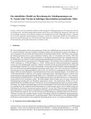
5 Numerical Examples
In order to illustrate the behavior of the proposed method, a few numerical examples are selected. In all of them
a simple softening function f(d) = e −d is used, which results in a semi-ductile behaviour. It is also possible to
include other forms of the softening functions, in order to describe more brittle behaviour.
5.1 Infinitely Long Pre-Cracked Brick Subjected to Tension
The first example is an infinitely long pre-cracked brick subjected to tension, applied as uniform displacement at
the ends of the specimen. Due to existing symmetries only one fourth of the system is analyzed. The geometry of
the problem together with the parameters utilized is given in the Figure 1.
47

material data
E [GPa] 18.0
ν 0.2
c d [MPa·mm 2 ] 1.0
β d [MPa] 1.0
r 1 [MPa] 0.01
γ 1 1.0
h [mm] 100
b [mm] 40
a [mm] 16
Figure 1. Geometry and material parameters of the pre-cracked brick test
Calculations are performed using the damage model given in (19) and (20). In the first part of the test, the behavior
of the local material model is investigated (presented in the Figure 2, left). Soon after the damage process starts,
the resulting system of equations becomes instable and can not be solved. Another typical characteristic of the
unregularized models involving softening phase is noticeable: strong mesh dependence of the obtained results,
since the inelastic processes tend to localize in a single element next to the crack tip. Therefore a failure occurs
significantly earlier in a refined mesh. In contrast to that, the gradient enhanced model can be used to perform the
calculation even very far in the softening range without large difficulties (Figure 2, right). Analyses performed
with 350, 1170 and 6240 elements result in almost identical curves. Hence the mesh dependence is removed as
well.
300
250
350 elements, local
1170 elements, local
6240 elements, local
600
500
350 elements
1170 elements
6240 elements
Resultant reaction Force [N]
200
150
100
Resultant reaction Force [N]
400
300
200
50
100
0
0
0 0.005 0.01 0.015 0.02 0.025 0.03 0.035 0.04
0 0.02 0.04 0.06 0.08 0.1 0.12 0.14 0.16
Displacement [mm]
Displacement [mm]
Figure 2. Load-displacement diagrams for the cracked brick problem using non-local and local damage model
The distribution of damage shows mesh-objectivity as well (taking into consideration that on a finer mesh a more
precise post-processing can be performed). That can be seen in Figure 3., where the distribution on the 350-element
mesh (Figure 3. left) and on the 1170-element mesh (Figure 3. right) is presented.
_________________
Damage Parameter
_________________
Damage Parameter
0.00E+00
0.00E+00
5.00E-01
1.00E+00
1.50E+00
2.00E+00
2.50E+00
3.00E+00
3.50E+00
4.00E+00
4.50E+00
5.00E+00
4.21E+00
0.00E+00
0.00E+00
5.00E-01
1.00E+00
1.50E+00
2.00E+00
2.50E+00
3.00E+00
3.50E+00
4.00E+00
4.50E+00
5.00E+00
4.27E+00
Time = 1.60E+02
Time = 1.60E+02
Figure 3. Distribution of the damage parameter d on 350 and 1170 element mesh at the end of the test
5.2 Infinitely Long Brick With a Circular Hole Subjected to Tension
The second example is an infinitely long brick with a circular hole subjected to tension, applied as in the previous
case in the form of uniform displacement at the ends of the specimen. The geometry of the problem together with
the utilized parameters is given in the Figure 4. Due to existing symmetries only one fourth of the system was
analyzed.
48

material data
E [GPa] 18.0
ν 0.2
c d [MPa·mm 2 ] 1.0
β d [MPa] 1.0
r 1 [MPa] 0.01
γ 1 1.0
Figure 4. Geometry and material parameters of the brick with a hole test
Calculations are performed using the damage model given in (19) and (20). The purpose of this calculation is to
show that the results obtained in the analyses are mesh objective, and to investigate the influence of the gradient
parameter c d on the structural behavior. In order to test the mesh objectivity, three simulations with increasingly
finer meshes (with 200, 800 and 1800 elements) are performed using the parameters given in the Figure 4. The
resulting force-displacement diagrams are presented in the Figure 5. It is obvious that the difference between the
three calculations is insignificant .
Resultant reaction Force [N]
800
700
600
500
400
300
200
100
200 elements
800 elements
1800 elements
0
0 0.05 0.1 0.15 0.2 0.25
Displacement [mm]
Figure 5. Load-displacement diagrams for the brick with a hole problem using non-local damage model
The value of the parameter c d signifies the degree of the regularization. Utilizing the gradient strategy the distribution
of the damage parameter is smoothed over some localization zone rather than allowing a localization to
take place at a single surface (line, point). Therefore, higher values of c d lead to the smoother solution for the
damage variable, and as a consequence wider activated zone around the onset of localization. A series of tests on
the 800-element mesh is performed in order to investigate the influence of the gradient parameter on the structural
behaviour and the results are presented in the Figures 6. and 7.
Figure 6. Influence of the gradient parameter c d on the load-displacement diagrams
49

For small values (0.01-0.1) of the gradient parameter the calculations cannot be advanced far into the softening
range due to numerical instabilities of the system of equations. But for values c d ≥ 0.5 the regularization is
successful, and we are able to complete the calculations without significant difficulties (Figure 6). It is obvious
that system response in the form of force-displacement diagram strongly depends on the value of c d . The difference
in the value of the limit loads obtained for the different gradient parameters is due to the width of the activated
zone. For higher c d the activated zone is wider (as it can be seen in the Figure 7., where the plots of the damage
distribution across the specimen for several values of the gradient parameter and for the denoted displacement are
given), leading to smoother distribution and consequently decreased value of damage, which finally causes lower
load-bearing capacity loss.
C d = 0.2
C d = 0.5
____________________
Material Damage [%]
____________________
Material Damage [%]
0.00E+00
0.00E+00
1.00E+01
2.00E+01
3.00E+01
4.00E+01
5.00E+01
6.00E+01
7.00E+01
8.00E+01
9.00E+01
1.00E+02
9.79E+01
0.00E+00
0.00E+00
1.00E+01
2.00E+01
3.00E+01
4.00E+01
5.00E+01
6.00E+01
7.00E+01
8.00E+01
9.00E+01
1.00E+02
8.90E+01
Time = 7.70E+01
7.80E+01
C d = 1.0
Time = 7.70E+01
7.80E+01
C d = 5.0
____________________
Material Damage [%]
____________________
Material Damage [%]
0.00E+00
0.00E+00
1.00E+01
2.00E+01
3.00E+01
4.00E+01
5.00E+01
6.00E+01
7.00E+01
8.00E+01
9.00E+01
1.00E+02
6.74E+01
0.00E+00
0.00E+00
1.00E+01
2.00E+01
3.00E+01
4.00E+01
5.00E+01
6.00E+01
7.00E+01
8.00E+01
9.00E+01
1.00E+02
2.36E+01
Time = 7.60E+01
7.80E+01
Time = 8.00E+01
7.80E+01
Figure 7. Influence of the gradient parameter c d on the damage distribution
5.3 Brazil Cylinder Test
The final example is a so-called Brazil cylinder test. This test is often used for the identification of the uniaxial
tensile strength of rock-like materials (especially concrete). As in the previous examples, existing symmetries
allow to analyze on only one fourth of the system. The geometry and the parameters are given in the Figure 8.
concrete cylinder
press plates
P
P d=12.7 mm
R= 0.1524 m
d= 0.0127 m
E= 26170 MPa
= 0.18
d
= 10 . MPa
2
C= d 0. 1MPamm
4
r1=
1. 7210
MPa
R
d
P
Figure 8. Geometry and material parameters of the Brazil cylinder test
h
R=152.4 mm
Since this test is normally used for tension-sensitive materials, a damage model sensitive to tension (given in
equations (21), (22) and (23)) is used in the calculations. Three calculations on increasingly finer meshes (675,
1200 and 2300 elements) are performed in order to investigate the stability of the numerical system and meshobjectivity.
The resulting force-displacement diagrams, together with the damage distribution obtained on a 2300-
element mesh in the post-peak regime, can be seen in Figure 9.
50

1 6 0 0 0 0
A p lie d re s u lta n t fo rc e [N ]
1 4 0 0 0 0
1 2 0 0 0 0
1 0 0 0 0 0
8 0 0 0 0
6 0 0 0 0
4 0 0 0 0
2 0 0 0 0
6 7 5 E le m e n ts
1 2 0 0 E le m e n ts
2 3 0 0 E le m e n ts
Material _________________________
Damage [%]
6.28E+01
1.00E+02
9.00E+01
8.00E+01
7.00E+01
6.00E+01
5.00E+01
4.00E+01
3.00E+01
2.00E+01
1.00E+01
0.00E+00
0.00E+00
0
0 ,0 0 0 ,0 1 0 ,0 2 0 ,0 3 0 ,0 4 0 ,0 5 0 ,0 6 0 ,0 7
D is p la c e m e n t [m m ]
Figure 9. Load-displacement diagrams and damage distribution for the Brazil test
Time = 5.10E-02
5.13E-02
The difference between the obtained results is obviously very small and the calculations in the softening range are
performed without significant difficulties. This implies that within the proposed method for gradient enhancement
a range of different damage models can be efficiently regularized.
6 Conclusions
In the present paper a method for the gradient enhancement of continuum damage models based on a two-field minimisation
of the enhanced free energy is presented. Several numerical examples involving different damage models
show that the method efficiently removes pathological mesh dependence together with the numerical difficulties
connected with the calculation in the softening range of the materials. In addition, the influence of the gradient
material parameter on the global response of the system, distribution of damage and the calculation procedure is
discussed.
Acknowledgments
The present study is supported by the German National Science Foundation (DFG) within the joint research project
SFB 526 ”Reology of Earth”, subproject B7: ”Rheological Response of Continental Crust to Thermal Pulses
Related to Magmatism and Volcanism”. This support is gratefully acknowledged.
References
Abu Al-Rub, R.; Voyiadjis, G.: A direct finite element implementation of the gradient-dependent theory. International
Journal for Numerical Methods in Engineering, 63, (2005), 603 – 629.
Bažant, Z.; Jirásek, M.: Nonlocal integral formulations of plasticity and damage: Survey of progress. Journal of
Engineering Mechanics, 128, (2002), 1119–1149.
de Borst, R.; Pamin, J.: Some novel developments in finite element procedures for gradient-dependent plasticity.
International Journal for Numerical Methods in Engineering, 39, (1996), 2477–2505.
Dimitrijevic, B.; Hackl, K.: A method for gradient enhancement of inelastic material models. In: M. Kojic; M. Papadrakakis,
eds., Procceedings of First South-East European Conference on Computational Mechanics, pages
191–197 (2006).
Hackl, K.: Generalized standard media and variational principles in classical and finite strain. Journal of the
Mechanics and Physics of Solids, 45, (1997), 667–688.
Lorentz, E.; Benallal, A.: Gradient constitutive relations: numerical aspects and application to gradient damage.
Computer Methods in Applied Mechanics and Engineering, 194, (2005), 5191–5220.
Makowski, J.; Hackl, K.; Stumpf, H.: The fundamental role of nonlocal and local balance laws of material forces
in finite elastoplasticity and damage mechanics. International Journal of Solids and Structures, 43, (2006), 3940
– 3959.
51

Nedjar, B.: Elastoplastic-damage modelling including the gradient of damage: formulation and computational
aspects. International Journal of Solids and Structures, 38, (2001), 5421 – 5451.
Peerlings, R.: Enhanced damage modeling for fracture and fatigue. Techische Universiteit Eindhoven, Eindhoven
(1999).
Peerlings, R.; de Borst, R.; Brekelmans, W.; Geers, M.: Gradient-enhanced damage modeling of concrete fracture.
Mechanics of Cohesive-Frictional Materials, 3, (1998), 323 – 342.
Peerlings, R.; Masart, T.; Geers, M.: A thermodynamically motivated implicit gradient damage framework and its
application to brick masonry cracking. Computer Methods in Applied Mechanics and Engineering, 193, (2004),
3403 – 3417.
Simo, J.; Ju, J.: Strain and stress based continuum damage models-i. formulation. International Journal of Solids
and Structures, 23, (1987), 821 – 840.
Simone, A.; Askes, H.; Peerlings, R.; Sluys, L.: Interpolation requirements for implicit gradient-enhanced continuum
damage models. Communications in Numerical Methods in Engineering, 19, (2003), 563 – 572.
Address: M. Sc. Bojan J. Dimitrijevic and Prof. Dr. rer. nat. Klaus Hackl, Institut für Mechanik, Ruhr Universität
Bochum, Universitätsstr. 150, D-44801 Bochum
email: Bojan.Dimitrijevic@rub.de; Klaus.Hackl@rub.de
52