Quasi-static Response of a Timoshenko Beam Loaded by an ...

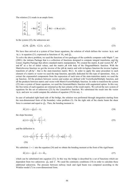
The relation (21) reads in an ample form:
⎡ )
⎢ )
⎢
⎢
)
⎢ )
⎣ ⎢
w b
l
ϕ b
l
⎤
⎥
⎥
⎥
M 0
⎥
Q 0 ⎦ ⎥ )
x = ) s
⎡ 0 ⎤
=Φ( s ) ⎢ ) l
ϕ
⎥
) ⎢ b ⎥
⎢ 0 ⎥
⎢ )
l
⎣ Q b ⎦
⎥
)
x = 0
In the system (22), the unknowns are:
)
ϕ b l (0),
)
s
+ ∫ Φ( ) s −τ ) b u(τ )dτ , (22)
0
)
Q b l (0), ) w b l ( ) s ), ϕ b l ( ) s ) . (23)
We have thus arrived at a system of four linear equations, the solution of which defines the vectors X(0) and
X( ) s ) in equation (21), expressed as functions of M )
0 and Q )
0 .
To solve the above problem, we used the functions of two packages of the symbolic computer code Maple 7, see
(2001): the inttrans Package that is a collection of functions designed to compute integral transforms, and the
Linear Algebra Package that allows standard matrix manipulation. We created the matrix A and vectors X T , X ’T
and b T as a list of initial values, and the matrix pI with help of the DiagonalMatrix function. With the
MatrixInverse function we got the inverse of the (pI-A) matrix and with invlaplace function the inverse Laplace
transform of (pI-A) -1 , that is the state-transition matrix Φ( x ) ) . In order to apply the same procedure to each
element of a matrix or vector we used the map function, specially dedicated for this type of operations. Also, to
extract the exponential components from the expression of each term of the state-transition matrix we used the
op function. All the products between vectors and scalars are defined with VectorScalarMultiply function, and
all the products between matrix and vector with MatrixVectorMultiply function. In order to transform the system
(22) into a system of linear equations, we used the GenerateMatrix function with augmented option. In this way
the free terms of each equation are returned as the last column of the result matrix. We solved the new system of
equations for the set of unknowns (23) by the LinearSolve function. We substituted the result into the vector
X(0) and now we could compute the solution of equation (19) for any ) x .
In case of unloaded right hand side of the bridge, the solution was performed through integration starting from
the non-dimensional form of the boundary value problem (3). On the right side of the elastic beam the shear
force is constant and equal to Q )
0 . Then, the bending moment is:
)
M b r ( ) x ) =− )
Q 0 ( )
L − ) x ), (24)
the slope becomes:
)
ϕ r b ( x ) ) = Q ) ⎛ )
0 L x ) )
x 2 ⎞
−
⎜ 2 ⎟ − C )
, (25)
⎝ ⎠
and the deflection is:
)
w r b ( ) x ) = ) ⎛
⎜
⎝
(26)
)
Q 0 L
)
x 2
2 − )
x 3
)
6 − L 3 ⎞
3 ⎟ − C ) ⎛
⎜
) x − L
) ⎞
⎟ + α Q ) ⎛ )
⎝ ⎠ 0
⎜ x − L
) ⎞
⎟ .
⎝ ⎠
⎠
We substitute ) x = ) s into the equation (24) and we obtain the bending moment at the front of the rigid beam:
)
M r b ( ) s ) =− Q )
0 ( L )
− s ) ) = M )
0 , (27)
which can be substituted into equation (21). In this way the bridge is described by a set of functions which are
dependent from two unknowns: Q )
0 and C )
. We used the continuity conditions (14) in order to calculate these
additional unknowns. The pressure between railway track and rigid beam was computed according to the
Winkler model (7) in a non-dimensional form.
84