Novel Three-Phase CM/DM Conducted Emissions Separator
Novel Three-Phase CM/DM Conducted Emissions Separator
Novel Three-Phase CM/DM Conducted Emissions Separator

Create successful ePaper yourself
Turn your PDF publications into a flip-book with our unique Google optimized e-Paper software.
<strong>Novel</strong> <strong>Three</strong>-<strong>Phase</strong> <strong>CM</strong>/<strong>DM</strong> <strong>Conducted</strong> <strong>Emissions</strong> <strong>Separator</strong><br />
M. L. Heldwein 1 , T. Nussbaumer 1 , F. Beck 2 and J. W. Kolar 1<br />
1<br />
Swiss Federal Institute of Technology (ETH) Zurich<br />
Power Electronic Systems Laboratory<br />
ETH Zentrum / ETL H23, Physikstrasse 3<br />
CH-8092 Zurich / SWITZERLAND / Europe<br />
heldwein@lem.ee.ethz.ch<br />
2<br />
Schaffner EMV AG<br />
Research and Technology<br />
Nordstrasse 11<br />
CH-4542 Luterbach / SWITZERLAND / Europe<br />
FBeck@schaffner.com<br />
Abstract — This paper presents two novel three-phase common<br />
mode/differential mode noise separation networks, a passive and an<br />
active network, to be used in EMC conducted emission measurements<br />
of three-phase equipment. The passive network is analyzed theoretically<br />
and a prototype is constructed. Its evaluation is presented<br />
through frequency response measurements and conducted emission<br />
tests performed on a three-phase motor drive and verifies that the<br />
network is capable of separating the common and differential mode<br />
information in a CE measurement condition.<br />
I. INTRODUCTION<br />
<strong>Three</strong>-phase conducted emission (CE) measurements are a major<br />
issue for developing high power electronic equipment that is connected<br />
to a commercial electric grid due to EMC concerns which are<br />
reflected in international and regional regulation. <strong>Three</strong>-phase power<br />
electronic systems, such as motor drives and high power rectifiers,<br />
must comply with these regulations. To achieve compliance the<br />
equipment must include filtering and other electromagnetic emission<br />
control strategies. The conceptualization and the dimensioning of<br />
these emission control techniques are being increasingly researched<br />
and as a result analytical and experimental tools are being developed<br />
to aid the design engineers. There, the qualitative and quantitative<br />
assessment of the noise modes, common (<strong>CM</strong>) and differential (<strong>DM</strong>)<br />
modes, is of great importance. The main objective of this work is to<br />
propose a device that can be integrated in a three-phase CE standard<br />
measurement system that allows the separate evaluation of <strong>CM</strong> and<br />
<strong>DM</strong> emission levels. This device is named the three-phase <strong>CM</strong>/<strong>DM</strong><br />
noise separator.<br />
Circuits that provide the discrimination of noise modes for singlephase<br />
systems have been presented in [1]-[6] and their operating<br />
principle is based on the fact that the summing and subtracting of<br />
two sensed voltages leads to the measurement of the distinct emission<br />
values for <strong>CM</strong> and <strong>DM</strong>. Other methods that use mathematical<br />
analysis through Fast Fourier Transformation [8] are used, provided<br />
that sampling rates are adequate and phase information is correctly<br />
computed.<br />
A three-phase measurement system capable of separately measuring<br />
both noise modes is proposed in [7] and it employs current<br />
transducers and hybrid junctions. However, the drawbacks of this<br />
system are that it does not fulfill all the specifications of CISPR 16<br />
and it requires a complex assembly for the test setup. In [8] another<br />
measurement technique is presented, which is suitable for high<br />
power levels, but it does not use a LISN and needs numerical treatment<br />
for the acquired data. Numerical models are presented in [9]<br />
which also allow for the <strong>CM</strong> and <strong>DM</strong> emission levels estimation but<br />
only if detailed model of the system is available. Another method is<br />
given in [10], which uses post mathematical processing in order to<br />
calculate the <strong>CM</strong>/<strong>DM</strong> emission values based on the noise propagation<br />
characteristics for the converter under consideration.<br />
In this paper, a novel hardware interface between a three-lines<br />
LISN and an EMC test receiver is proposed, thus allowing a realtime<br />
direct measurement of <strong>DM</strong> and <strong>CM</strong> emission levels in a typical<br />
CISPR 16 specified setup [11], [12].<br />
A<br />
B<br />
C<br />
4 µF<br />
250 µH 50 µH<br />
8 µF<br />
Mains frequency<br />
decoupling paths<br />
250 nF<br />
High frequency<br />
coupling paths<br />
a<br />
b<br />
c<br />
EUT<br />
High frequency<br />
simplified equivalent<br />
EUT<br />
(HF noise source)<br />
i a<br />
i b<br />
i c<br />
a<br />
b<br />
c<br />
u <strong>DM</strong>,a<br />
u <strong>DM</strong>,b<br />
u <strong>DM</strong>,c<br />
PE<br />
10 Ω<br />
3 lines LISN<br />
5 Ω<br />
a'<br />
b'<br />
c'<br />
PE<br />
50 Ω<br />
u a<br />
u b<br />
u c<br />
i <strong>CM</strong><br />
PE<br />
u <strong>CM</strong><br />
Test receiver input and<br />
LISN terminations<br />
50 Ω<br />
Test receiver input and<br />
50 Ω terminations<br />
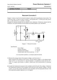
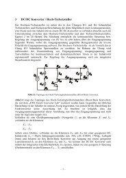
Fig.1: Typical three-phase CE measurement setup schematic and high frequency simplified circuit.
In Section II a short discussion on CE measurements in threephase<br />
systems and the relationships between measured voltages and<br />
noise modes are presented, and this provides the analytical basis for<br />
the <strong>CM</strong>/<strong>DM</strong> separation in three-phase systems. Two basic circuit topologies<br />
– a passive and an active one – for three-phase <strong>CM</strong>/<strong>DM</strong><br />
separation networks are proposed in Section III and the passive one<br />
is analyzed. A hardware realization of the passive circuit is discussed<br />
in Section IV and experimental results, illustrating the<br />
performance of the hardware prototype, are given in Section V.<br />
II. THREE-PHASE CONDUCTED EMISSION MEASUREMENTS<br />
AND NOISE COMPONENTS<br />
In order to evaluate equipment for compliance to CE noise limits a<br />
Line Impedance Stabilization Network (LISN) is usually utilized.<br />
Basically, the LISN has to fulfill the following three functions: defining<br />
the mains impedance in order to standardize the measurement;<br />
decoupling the low frequency AC power supply voltage from the<br />
measurement equipment and; providing a high frequency coupling<br />
path between the equipment under test (EUT) and a measurement<br />
test receiver.<br />
The impedance curve of a LISN is defined by EMC standards, for<br />
instance as in CISPR 16 [13]. A typical realization of a three-phase<br />
LISN circuit is depicted in Fig.1. For the CE measurement process a<br />
test receiver with 50Ω input impedance is connected to one of the<br />
LISN channels while the remaining two LISN ports are terminated<br />
with 50Ω creating symmetric measurement conditions.<br />
Assuming, at high frequencies, an ideal decoupling from the EUT<br />
to the mains and a perfect coupling with the test receiver, which is<br />
the case for the circuit of Fig.1 in a simplified consideration, the<br />
equivalent high frequency circuit (Fig.1) is obtained and used in the<br />
following analysis. There, the input ports a, b and c of the EUT are<br />
directly connected to the input ports of the test receiver what means<br />
that all high frequency noise from the EUT is coupled to the test receiver,<br />
while the mains ports A, B and C are separated from the EUT.<br />
The measured voltages u i (with i = a, b, c) at the test receiver 50 Ω<br />
sensing resistors comprise both a differential mode and a common<br />
mode component<br />
u = u + u . (1)<br />
i <strong>DM</strong>,<br />
i <strong>CM</strong><br />
These two components are caused by the three differential mode<br />
currents i <strong>DM</strong>,i and a common mode current i <strong>CM</strong> circulating between<br />
the EUT and the test receiver. For a symmetric distribution of i <strong>CM</strong><br />
between the three phases the currents i i flowing to the test receiver<br />
input ports are<br />
i<strong>CM</strong><br />
ii<br />
= i<strong>DM</strong>,<br />
i + . (2)<br />
3<br />
Due to the fact that the sum of the differential mode currents is,<br />
per definition, equal to zero<br />
i + i + i = , (3)<br />
<strong>DM</strong> , a <strong>DM</strong> , b <strong>DM</strong> , c 0<br />
the sum of the currents to the test receiver equals the common mode<br />
current<br />
ia + ib + ic = i<strong>CM</strong><br />
. (4)<br />
Therefore, the common mode voltage can be evaluated by the<br />
summation of the measured voltages<br />
u + u + u = R⋅ i + i + i = R⋅ i = ⋅ u . (5)<br />
u <strong>DM</strong>,a<br />
u <strong>DM</strong>,b<br />
u <strong>DM</strong>,a<br />
u <strong>DM</strong>,b<br />
u <strong>DM</strong>,c<br />
u <strong>CM</strong><br />
R<br />
R<br />
( ) 3<br />
a b c a b c <strong>CM</strong> <strong>CM</strong><br />
For evaluating the differential mode components the common<br />
mode part has to be eliminated. This can be achieved directly by the<br />
subtraction of two test receiver voltages<br />
u − u = u − u . (6)<br />
a b <strong>DM</strong>, a <strong>DM</strong>,<br />
b<br />
With (5) and (6) one can realize that a separated evaluation of the<br />
common and differential mode components in a three-phase system<br />
is achievable through proper mathematical formulation. This results<br />
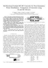
in the development of electrical networks as presented in Fig.2.<br />
III. THREE-PHASE <strong>CM</strong>/<strong>DM</strong> NOISE SEPARATION NETWORKS<br />
In order to practically implement the mathematical formulation<br />
given in the previous section and properly separate both noise<br />
modes using an electrical network two circuit topologies are proposed<br />
in Fig.2 [14]. Fig.2(a) shows a passive solution which is<br />
R 3<br />
Tr a<br />
Tr b<br />
Tr c<br />
u <strong>CM</strong>,out<br />
u <strong>DM</strong>,c<br />
R 3 . R 1<br />
u <strong>CM</strong><br />
R 1<br />
R<br />
R<br />
R<br />
R 2<br />
R 2<br />
R 2<br />
R 2<br />
u <strong>DM</strong>,out,a<br />
u <strong>DM</strong>,out,a<br />
u <strong>DM</strong>,out,a<br />
_<br />
+<br />
_<br />
+<br />
R 2<br />
R 2<br />
_<br />
+<br />
u <strong>CM</strong><br />
2<br />
-u <strong>DM</strong>,a<br />
-u <strong>DM</strong>,b<br />
-u <strong>DM</strong>,c<br />
(b)<br />
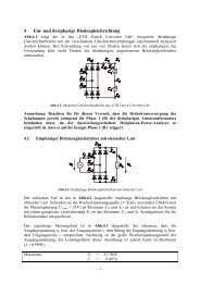
Fig.2: <strong>Three</strong>-phase <strong>CM</strong>/<strong>DM</strong> noise separator proposals [14]. (a) Passive solution.<br />
(b) Active solution.<br />
(a)
analyzed in detail in this paper. The circuit of Fig.2(b) uses active<br />
elements and will be analyzed in a further publication. In the figures<br />
the high frequency noise components are depicted by a common<br />
mode voltage source u <strong>CM</strong> and three differential mode voltage<br />
sources u <strong>DM</strong>,a , u <strong>DM</strong>,b and u <strong>DM</strong>,c .<br />
A network that makes use of active circuits would require amplifiers<br />
with very large bandwidths and high power supply rejection<br />
ratios, and the design of a suitable amplifier power supply. However,<br />
the active solution would provide well defined input impedances<br />
and a good control of the insertion loss allowing required adjustments<br />
to be done easily.<br />
The passive solution comprises of three transformers Tr a , Tr b and<br />
Tr c with star-connected primaries, delta-connected secondaries and<br />
one-to-one turns ratio. The primary side star-point is connected to<br />
the ground via a resistor R/3 while the secondaries are terminated by<br />
resistors R.<br />
The mathematical analysis of the circuit helps to clarify the noise<br />
separation effect. Equations (7) and (8) are obtained from the circuit.<br />
u + u − u = u<br />
(7)<br />
<strong>CM</strong> <strong>DM</strong>i , <strong>DM</strong>outi , , <strong>CM</strong>out ,<br />
3<br />
u<strong>DM</strong> , out,<br />
i = 0<br />
i=<br />
1<br />
∑ (8)<br />
According to the definition of the differential mode voltage<br />
sources and based on the fact that the termination impedances R a , R b<br />
and R c are balanced it follows that:<br />
3<br />
∑ u<strong>DM</strong> , i = 0<br />
(9)<br />
i=<br />
1<br />
The summing of the three equations included in (7) leads to equation<br />
(10).<br />
u<br />
<strong>CM</strong><br />
= u<br />
(10)<br />
<strong>CM</strong> , out<br />
u<br />
= u<br />
(11)<br />
<strong>DM</strong>, i <strong>DM</strong>outi , ,<br />
Based on (10) and (11) it is clear that the proposed network provides<br />
in its output ports the values for the differential and common<br />
mode voltages.<br />
Another relevant issue for the measurement setup is the value of<br />
the input impedances of the network since the CE measurements<br />
with a LISN usually demand 50 Ω balanced sensing resistors. Since<br />
the network is symmetric the analysis of the input impedances is<br />
done with the help of Fig.3 for only one of the inputs.<br />
By solving the circuit equations one gets to equation (12).<br />
u a R<br />
9<br />
a ⋅R b ⋅R c ⋅R<br />
= ⋅<br />
<strong>CM</strong><br />
(12)<br />
ia Ra ⋅Rb⋅ Rc + R<strong>CM</strong> ⋅⎡⎣4<br />
⋅Rb⋅ Rc + Ra ⋅ ( Rb + Rc)<br />
⎤⎦<br />
In order to have a balanced circuit the resistors R i have to be made<br />
equal:<br />
Ra = Rb = Rc<br />
= R<br />
(13)<br />
Replacing (13) in (12) results in (14).<br />
ua<br />
9<br />
Rin,<br />
a = =<br />
(14)<br />
i 6 1<br />
a +<br />
R R<br />
Since the <strong>DM</strong> output ports will be sensed with the resistance R<br />
and this will be done in a test receiver with an input resistance of 50<br />
Ω it is desirable that the input resistance present the same value, i.e.<br />
R in = R. Solving (14) gives (15):<br />
R<br />
R <strong>CM</strong> = (15)<br />
3<br />
Based on the presented analytical equations it is certain that the<br />
proposed network is able to perform the separation of <strong>CM</strong> and <strong>DM</strong><br />
conducted emission levels in a standard measurement setup.<br />
<strong>CM</strong><br />
By replacing (10) in (7) gives (11):<br />
u <strong>DM</strong> , a<br />
Tr a<br />
L a<br />
i S<br />
R<br />
u <strong>DM</strong>,<br />
out,a<br />
i a<br />
1:1<br />
u <strong>DM</strong> , b<br />
Tr b<br />
L b<br />
R in,a<br />
u a<br />
R a<br />
u <strong>DM</strong>,out,a<br />
R<br />
u <strong>DM</strong>,<br />
out,b<br />
i b<br />
1:1<br />
i c 1:1<br />
R cm<br />
u <strong>CM</strong>,out<br />
R b<br />
R c<br />
u <strong>DM</strong>,out,a<br />
u <strong>DM</strong>,out,a<br />
u <strong>CM</strong><br />
u <strong>DM</strong> , c<br />
Noise source<br />
( LISN / AMN )<br />
1<br />
3<br />
R<br />
Tr c<br />
u <strong>CM</strong>,out<br />
Common mode<br />
measurement<br />
L c<br />
R = 50 Ω<br />
R<br />
u <strong>DM</strong>,<br />
out,c<br />
Differential mode<br />
measurements<br />
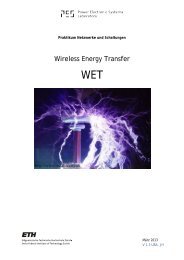
Fig.3: Circuit used for the calculation of the input impedances to ground.<br />
Fig.4: Circuit schematic of the three-phase <strong>CM</strong>/<strong>DM</strong> noise separator.
LISN output voltage [V]<br />
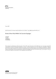
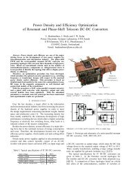
Fig.5: <strong>Three</strong>-phase <strong>CM</strong>/<strong>DM</strong> separator prototype photograph. Overall dimensions:<br />
12.0x9.5x5.7 cm (4.75x3.75x2.25 in.).<br />
IV. THREE-PHASE <strong>CM</strong>/<strong>DM</strong> NOISE SEPARATOR REALIZATION<br />
In order to implement the three-phase <strong>CM</strong>/<strong>DM</strong> noise separator<br />
presented in the previous section the schematic in Fig.4 is used. The<br />
separator is specified to be used in a standard CISPR 16 CE test<br />
setup using a typical (50 µH + 5 Ω) // 50 Ω V-network LISN and applying<br />
input line-to-line voltages of 400 V / 50 Hz.<br />
The noise separator is built with the network formed by the transformers<br />
Tr a , Tr b and Tr c and the inductors L a , L b and L c . Employing<br />
R = 50 Ω ensures an equivalent resistance of the noise separator inputs<br />
to ground of 50 Ω and allows the measurement of the <strong>CM</strong> and<br />
<strong>DM</strong> noise voltages directly from the respective output ports. For<br />
measuring a differential mode noise voltage the corresponding output<br />
is connected to the input of the test receiver (input impedance of<br />
50 Ω) after removing the explicit resistive termination. Considering<br />
parasitic coupling capacitances of the transformers the measurement<br />
with reference to ground causes an asymmetry of the circuit which<br />
could result in a transformation of <strong>CM</strong> into <strong>DM</strong> noise. In order to<br />
achieve a higher common mode rejection ratio (<strong>CM</strong>RR), therefore<br />
common mode inductors L a , L b and L c , ensuring equal impedances<br />
of the transformer output terminals against ground for high frequencies,<br />
are inserted into the differential mode outputs. A photo of a<br />
first practical realization of the three-phase <strong>CM</strong>/<strong>DM</strong> noise separator<br />
is shown in Fig.5.<br />
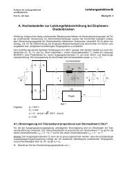
Flux density [T]<br />
0.3<br />
0.2<br />
0.1<br />
0.0<br />
-0.1<br />
-0.2<br />
-0.3<br />
1.0<br />
0.5<br />
0.0<br />
-0.5<br />
-1.0<br />
0 4 8 12 16 20<br />
Time [ms]<br />
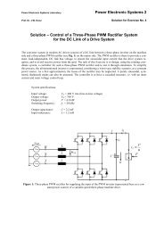
Fig.6: Calculated flux density in the designed transformers Tr a , Tr b and Tr c , for a<br />
simulated LISN output voltage when feeding a three-phase 5 kW rectifier.<br />
In order to construct the transformers in the separator some requirements<br />
must be fulfilled, namely: the 50 Hz component present<br />
in the LISN output and the maximum <strong>CM</strong> signal levels should not<br />
cause the saturation of the core; leakage inductance must be small in<br />
order not to influence the gains; primary to secondary capacitance<br />
values should also be as small as possible in order to prevent <strong>CM</strong><br />
paths to the secondary; good coupling should be guaranteed for low<br />
and high frequencies. Aiming for these characteristics the material<br />
VITROPERM 500F from Vacuumschmelze GmbH (VAC) was chosen,<br />
presenting a high maximum saturation flux density (B max ≅1.2 T)<br />
and good high frequency characteristics. The transformer is built<br />
with a VAC 25x16x10–T6000-6-L2025-W380 core with 10:10 turns<br />
of twisted insulated wires. Fig.6 shows a calculation result for the<br />
flux density in the core for the designed transformers Tr a , Tr b and<br />
Tr c when the LISN is feeding a three-phase rectifier supplying 5 kW<br />
and switching at 20 kHz. The <strong>CM</strong> chokes in the separator prototype<br />
are built with the same core material as the transformers using a<br />
smaller core (VAC 12.5x10x5–T6000-6-L2012-W498), and presenting<br />
a <strong>CM</strong> inductance around 1 mH.<br />
For applying the separator, a three or four line LISN must allow<br />
simultaneous access to all three-phase output ports. In case this is<br />
not possible, three individual single-phase LISNs could be employed.<br />
All asymmetries presented in the test circuit composed of<br />
the LISN and the noise separator will influence the measurements,<br />
especially in the higher frequency range and should be avoided.<br />
V. EXPERIMENTAL EVALUATION<br />
Some of the frequency response characteristics of the prototype<br />
were measured with a impedance and network analyzer in order to<br />
evaluate the design. These measurements were performed with 50 Ω<br />
input and output impedances. The most significant results of these<br />
measurements are shown in Fig.7. The insertion loss (calculated<br />
from the measured attenuation using the 50 Ω source/sense setups<br />
shown in Fig.7) curves for the three <strong>DM</strong> channels are quite similar<br />
and only one is presented in Fig.7(a) where the presented -3 dB cutoff<br />
frequency is higher than 20 MHz and good symmetry amongst<br />
the channels is observed. In Fig.7(b) the gain between a measured<br />
<strong>CM</strong> output voltage and a <strong>CM</strong> input signal is plotted and again a flat<br />
band up to more than 20 MHz is observed. As the noise separator is<br />
intended to discriminate common and differential modes it is important<br />
to check how good the attenuation of the other noise<br />
components is, for instance, when measuring a <strong>CM</strong> signal the influence<br />
of the <strong>DM</strong> channels is needed to be known. This can be<br />
evaluated through the measurement of the differential mode rejection<br />
ratio (<strong>DM</strong>RR) of all channels and of the common mode<br />
rejection ratio (<strong>CM</strong>RR) for the <strong>DM</strong> channels. As the <strong>DM</strong>RRs of the<br />
<strong>DM</strong> channels is very similar it is presented in Fig.7(c) using only<br />
one measurement that was performed for the <strong>DM</strong> output port C with<br />
the input signal applied between input ports A and B. The <strong>DM</strong>RRs<br />
of the <strong>CM</strong> port are shown in Fig.7(d)(e)(f) and for all cases is higher<br />
than 70 dB at 150 kHz and higher than 25 dB up to 30 MHz. The<br />
<strong>CM</strong>RR of the <strong>DM</strong> output ports is presented in Fig.7(g)(h)(i) show-
Source Measurement<br />
V 50 Ω<br />
50 Ω<br />
~<br />
<strong>CM</strong>,out<br />
a <strong>DM</strong>,out,a<br />
b <strong>DM</strong>,out,b<br />
c<br />
<strong>DM</strong>,out,c<br />
Network analyzer<br />
Noise separator<br />
Source Measurement<br />
V 50 Ω<br />
50 Ω<br />
~<br />
a<br />
b<br />
<strong>CM</strong>,out<br />
25 Ω<br />
<strong>DM</strong>,out,a<br />
<strong>DM</strong>,out,b<br />
Source Measurement<br />
V 50 Ω<br />
50 Ω<br />
~<br />
<strong>CM</strong>,out<br />
a <strong>DM</strong>,out,a<br />
b <strong>DM</strong>,out,b<br />
c<br />
<strong>DM</strong>,out,c<br />
c<br />
<strong>DM</strong>,out,c<br />
Network analyzer<br />
Noise separator<br />
Network analyzer<br />
Noise separator<br />
(a) <strong>DM</strong> insertion loss for channel a (b) <strong>CM</strong> insertion loss (c) <strong>DM</strong>RR for <strong>DM</strong> output port c<br />
(input signal: ports a and b)<br />
Source Measurement<br />
V 50 Ω<br />
50 Ω<br />
~<br />
a<br />
b<br />
<strong>CM</strong>,out<br />
<strong>DM</strong>,out,a<br />
<strong>DM</strong>,out,b<br />
Source Measurement<br />
V 50 Ω<br />
50 Ω<br />
~<br />
a<br />
b<br />
<strong>CM</strong>,out<br />
<strong>DM</strong>,out,a<br />
<strong>DM</strong>,out,b<br />
Source Measurement<br />
V 50 Ω<br />
50 Ω<br />
~<br />
<strong>CM</strong>,out<br />
a <strong>DM</strong>,out,a<br />
b <strong>DM</strong>,out,b<br />
Network analyzer<br />
c <strong>DM</strong>,out,c<br />
Noise separator<br />
Network analyzer<br />
c <strong>DM</strong>,out,c<br />
Noise separator<br />
Network analyzer<br />
c <strong>DM</strong>,out,c<br />
Noise separator<br />
(d) <strong>DM</strong>RR for <strong>CM</strong> output port<br />
(input signal: ports a and b)<br />
(e) <strong>DM</strong>RR for <strong>CM</strong> output port<br />
(input signal: ports b and c)<br />
(f) <strong>DM</strong>RR for <strong>CM</strong> output port<br />
(input signal: ports a and c)<br />
Source Measurement<br />
V 50 Ω<br />
50 Ω<br />
~<br />
a<br />
b<br />
<strong>CM</strong>,out<br />
<strong>DM</strong>,out,a<br />
<strong>DM</strong>,out,b<br />
Source Measurement<br />
V 50 Ω<br />
50 Ω<br />
~<br />
a<br />
b<br />
<strong>CM</strong>,out<br />
<strong>DM</strong>,out,a<br />
<strong>DM</strong>,out,b<br />
Source Measurement<br />
V 50 Ω<br />
50 Ω<br />
~<br />
a<br />
b<br />
<strong>CM</strong>,out<br />
<strong>DM</strong>,out,a<br />
<strong>DM</strong>,out,b<br />
c<br />
<strong>DM</strong>,out,c<br />
c<br />
<strong>DM</strong>,out,c<br />
c<br />
<strong>DM</strong>,out,c<br />
Network analyzer<br />
Noise separator<br />
Network analyzer<br />
Noise separator<br />
Network analyzer<br />
Noise separator<br />
(g) <strong>CM</strong>RR for <strong>DM</strong> output port <strong>DM</strong>,out,a (h) <strong>CM</strong>RR for <strong>DM</strong> output port <strong>DM</strong>,out,b (i) <strong>CM</strong>RR for <strong>DM</strong> output port <strong>DM</strong>,out,c<br />
Fig.7: Measured frequency characteristics for the <strong>CM</strong>/<strong>DM</strong> noise separator. All ordinate axes present 10 dB per division. Frequency range: 150 kHz to 30 MHz.<br />
ing around 50 dB in the lower frequency range and being around 20<br />
dB at 10 MHz. The measured frequency characteristics show that<br />
the noise separation network performs its task mainly in the frequency<br />
range up to 10 MHz. However, a better performance for<br />
higher frequencies is desirable so that rejection ratios in the order of<br />
30 dB at 30 MHz guarantee a clear separation of the noise modes.<br />
This could be achieved with a more symmetrical layout and components<br />
with improved HF performance.<br />
<strong>Conducted</strong> emission measurements as specified in CISPR 16 were<br />
performed utilizing a setup as shown in Fig.9 in order to give an example<br />
for the use of the three-phase <strong>CM</strong>/<strong>DM</strong> separator. The EUT<br />
was a regenerative drive feeding a 10 kW motor. The test conditions<br />
were as follows: input voltages U in =400V / 50Hz; output power P out =<br />
5 kW. The LISN conforms with CISPR 16, is constructed to operate<br />
from 2 kHz to 30 MHz and is presented in [15]. The access to all<br />
output ports is available, thus guaranteeing that the three-phase<br />
<strong>CM</strong>/<strong>DM</strong> noise separator can be used.<br />
Fig.8 shows the acquired data for three measurements done within<br />
the same operating conditions, one without the noise separator<br />
Fig.8(a), the second showing the measured emission levels sensed in<br />
one of the <strong>DM</strong> channels with the presented network Fig.8(b) and the<br />
last one depicts the measurement performed in the <strong>CM</strong> output port.<br />
From the measurements one can see that there is a large difference<br />
between the levels of <strong>DM</strong> and <strong>CM</strong> emissions in the lower frequency<br />
range with the <strong>DM</strong> emissions being much higher than the <strong>CM</strong> ones<br />
up to5 MHz. This indicates the necessity of higher <strong>DM</strong> attenuation<br />
at this frequency range. It also shows how much attenuation is required<br />
and this allows an appropriate filter to be designed. With this<br />
example the main purpose of the separator network, which is
SGL<br />
Det<br />
AV Trd<br />
30DB<br />
Det<br />
AV Trd<br />
30DB_<strong>DM</strong><br />
Det<br />
AV Trd<br />
30DB_<strong>CM</strong><br />
Att 10 dB AUTO<br />
ResBW 9 kHz<br />
Att 10 dB AUTO<br />
ResBW 9 kHz<br />
Att 10 dB AUTO<br />
ResBW 9 kHz<br />
INPUT 2<br />
Meas T 100 ms Unit<br />
dBV<br />
INPUT 2<br />
Meas T 100 ms Unit<br />
dBV<br />
INPUT 2<br />
Meas T 100 ms Unit<br />
dBV<br />
100<br />
100_QP<br />
1 MHz 10 MHz<br />
100<br />
100_QP<br />
1 MHz 10 MHz<br />
100<br />
100_QP<br />
1 MHz 10 MHz<br />
90 100_AV<br />
90 100_AV<br />
90 100_AV<br />
SGL<br />
SGL<br />
80<br />
80<br />
80<br />
70<br />
1MA<br />
70<br />
1MA<br />
70<br />
1MA<br />
60<br />
3AV<br />
60<br />
3AV<br />
60<br />
3AV<br />
50<br />
50<br />
50<br />
40<br />
40<br />
40<br />
30<br />
30<br />
30<br />
20<br />
20<br />
20<br />
10<br />
10<br />
10<br />
07.Sep 2004 07:04 Schaffner EMV AG<br />
0<br />
150 kHz 30 MHz<br />
07.Sep 2004 06:42 Schaffner EMV AG<br />
0<br />
150 kHz 30 MHz<br />
07.Sep 2004 07:01 Schaffner EMV AG<br />
0<br />
150 kHz 30 MHz<br />
Date: 7.SEP.2004 07:04:13<br />
Date: 7.SEP.2004 06:42:45<br />
Date: 7.SEP.2004 07:01:32<br />
(a) Direct LISN measurement (phase A) (b) <strong>DM</strong> separator output (phase A) (c) <strong>CM</strong> separator output<br />
Fig.8: Measurements performed with and without the noise separator. Axes: 0 to 100 dBmV and 150 kHz to 30 MHz. Upper curves: quasi-peak measurement as specified<br />
in CSIPR 16. Lower curves: average detection measurement. (a) Measurements applying directly a LISN; (b) Measurements performed in one noise separator <strong>DM</strong><br />
output port;(c) Measurements from the noise separator <strong>CM</strong> output port.<br />
acquiring information for filter designs and troubleshooting of<br />
power converters, is proved through experimental results.<br />
Test receiver<br />
3-φ <strong>CM</strong>/<strong>DM</strong> separator<br />
Mains<br />
a<br />
b<br />
c<br />
LISN<br />
EUT<br />
(three-phase motor drive)<br />
Fig.9: Test setup for the conducted emission measurements using the proposed<br />
three-phase <strong>CM</strong>/<strong>DM</strong> noise separation passive network.<br />
VI. CONCLUSIONS<br />
This paper has presented two novel three-phase <strong>DM</strong>/<strong>CM</strong> separation<br />
networks that are intended to be used in the evaluation of noise<br />
sources, which will help in the design and troubleshooting of electromagnetic<br />
emission control systems for electronic equipment. One<br />
network is an arrangement of passive components while the other is<br />
based on the use of active circuits. The operating principle and characteristics<br />
of the passive network were discussed and experimentally<br />
verified. <strong>Conducted</strong> emission measurements were successfully performed<br />
in a three-phase electric motor drive using the separator<br />
indicating the noise levels and dominating modes. This information<br />
could be employed to design the <strong>CM</strong> and <strong>DM</strong> stages of an EMC filter.<br />
REFERENCES<br />
[1] Paul, C.R.; Hardin, K.B.: Diagnosis and reduction of conducted noise<br />
emissions. IEEE Transactions on Electromagnetic Compatibility, Vol. 30,<br />
No. 4, pp. 553-560 (1988).<br />
[2] Nave, M.J.: A <strong>Novel</strong> Differential Mode Rejection Network fo <strong>Conducted</strong><br />
<strong>Emissions</strong> Diagnostics. IEEE 1989 National Symposium on Electromagnetic<br />
Compatibility, Denver, USA, 23-25 May, pp. 223-227 (1989).<br />
[3] Nave, M. J.: Power Line Filter Design for Switched-Mode Power Supplies.<br />
New York (NY), USA: Van Nostrand Reinhold; 1991.<br />
[4] Guo, T., Chen, D.Y., and Lee, F.C.: Separation of the Common-Modeand<br />
Differential-Mode-<strong>Conducted</strong> EMI Noise. IEEE Transactions on Power<br />
Electronics, Vol. 11, No. 3, pp. 480-488 (1996).<br />
[5] See, K.Y.: Network for <strong>Conducted</strong> EMI Diagnosis. Electronics Letters, Vol.<br />
35, Issue: 17, 19 Aug, pp. 1446-1447 (1999).<br />
[6] Mardiguian, M. and Raimbourg, J.: An Alternate, Complementary<br />
Method for Characterizing EMI Filters. . IEEE International Symposium on<br />
Electromagnetic Compatibility, Vol. 2, 2-6 Aug, pp. 882-886 (1999).<br />
[7] De Bonitatibus, A.; De Capua, C.; Landi, C.: A New Method for <strong>Conducted</strong><br />
EMI Measurements on <strong>Three</strong> <strong>Phase</strong> Systems. Proceedings of the 17th<br />
IEEE Instrumentation and Measurement Technology Conference IMTC<br />
2000, Baltimore, Maryland, USA, 1-4 May, Vol. 1, pp. 461-464 (2000).<br />
[8] Ran, L., Clare, J.C., Bradley, K.J. and Christopoulos, C.: Measurement<br />
of <strong>Conducted</strong> Electromagnetic <strong>Emissions</strong> in PWM Motor Drive Systems<br />
Without the Need for a LISN. IEEE Transactions on Electromagnetic Compatibility,<br />
Vol. 41, No. 1, pp. 50-55 (1999).<br />
[9] Ran, L., Gokani, S., Clare, J.C., Bradley, K.J. and Christopoulos, C.:<br />
<strong>Conducted</strong> Electromagnetic <strong>Emissions</strong> in Induction Motor Drive Systems<br />
Part I: Time Domain Analysis and Identification of Dominant Modes. IEEE<br />
Transactions on Power Electronics, Vol. 13, No. 4, pp. 757-767 (1998).<br />
[10] Shen, W., Wang, F. and Boroyevich, D.: Definition and Acquisition of <strong>CM</strong><br />
and <strong>DM</strong> EMI Noise for General-Purpose Adjustable Speed Motor Drives.<br />
Proceedings of the 2004 Annual Power Electronics Seminar at Virginia<br />
Tech, Blacksburg (VA), USA, 18-20 April, pp. 16-20 (2004).<br />
[11] Nussbaumer, T., Heldwein, M.L., and Kolar J.W., Differential Mode<br />
EMC Input Filter Design for a <strong>Three</strong>-<strong>Phase</strong> Buck-Type Unity Power Factor<br />
PWM Rectifier. Proceedings of the 4th International Power Electronics and<br />
Mo-tion Control Conference, Xian, China, Aug. 14 – 16, 2004, pp. 1521-<br />
1526.<br />
[12] Heldwein, M.L. , Nussbaumer, T. , and Kolar, J.W.: Differential Mode<br />
EMC Input Filter Design for <strong>Three</strong>-<strong>Phase</strong> AC-DC-AC Sparse Matrix PWM<br />
Converters. Proceedings of the 35th IEEE Power Electronics Specialists<br />
Conference, Aachen, Germany, June 20 - 25, CD-ROM, ISBN: 07803-<br />
8400-8 (2004).<br />
[13] IEC International Special Committee on Radio Interference –<br />
C.I.S.P.R. (1977): C.I.S.P.R Specification for Radio Interference Measuring<br />
Apparatus and Measurement Methods – Publication 16. Geneve, Switzerland:<br />
C.I.S.P.R.<br />
[14] Kolar, J.W., and Ertl, H.: Vorrichtung zur Trennung der<br />
Funkstörspannungen dreiphasiger Stromrichtersysteme in eine Gleich- und<br />
eine Gegentaktkomponente (in German). Swiss Patent Application, March<br />
2004.<br />
[15] Beck, F., Measurements of <strong>Conducted</strong> Voltage in the Low-Frequency Range<br />
from 2 kHz to 30 MHz for High-Current I ndustrial applications with regeneration<br />
drives, IEEE EMC 2004 Santa Clara, August 2004.