Ab_init stress perturbation theory - Department of Physics and ...

Implementation of the Strain
Perturbation in ABINIT
D. R. Hamann, 1,2,3 Xifan Wu 1
David Vanderbilt, 1 Karin Rabe, 1
1
Department of Physics and Astronomy, Rutgers University, Piscataway, NJ
2
Bell Laboratories, Lucent Technologies, Murray Hill, NJ
3
Mat-Sim Research LLC, Murray Hill, NJ
Supported by The Center for Piezoelectrics by Design, ONR grant N00014-01-1-0365
and Mat-Sim Research, www.mat-simresearch.com
Mat-Sim
Research

Overview
• Goal: Direct calculation of the elastic and piezoelectric tensors and
related quantities
• Strain and the Abinit reduced-coordinate formulation
• Brief review of density functional perturbation theory
• Response function (RF) code organization
• Development process design
• Special issues: nonlocal pseudopotentials, symmetry, non-linear core
corrections, cutoff smoothing, metals
• Using: new input and output
• Atom coordinate relaxation and anaddb post processing
• Future development issues
• (Appendix)

Strain tensor h ab as a perturbation
• Strain really only changes the positions of the atomic (pseudo)potentials,
cell
V () r = V ( r-τ -R) ⎯⎯→ V () r = V [ r-( 1+ η) ⋅τ- ( 1 + η) ⋅R].
ext
∑∑
τ
η ext
R τ R τ
cell
∑∑
• However, this causes unique problems for perturbations expansions:
– Viewed in terms of the infinite lattice, the strain perturbation can never be
small.
– From the point of view of a single unit cell, strain changes the periodic
boundary conditions, so wave functions of the strained lattice cannot be
expanded in terms of those of the unstrained lattice.
• Strain appears to be qualitatively different from other perturbations such
as periodicity-preserving atomic displacements
τ

Strain tensor h ab as a perturbation, continued
• Existing formulation (1)
– Introduce fictitious strained self-consistent Hamiltonian obtained by a scale
transformation of the unstrained Hamiltonian,
H!
!
∇= ⎡
⎣ + ⋅ + ⋅∇⎤
⎦
η
−1
SCF
(, r ) HSCF
(1 η) r,(1 η)
H η
SCF
H!
η
– obeys the same boundary conditions as the strained Hamiltonian
– has the same spectrum unstrained Hamiltonian, and a simply related
SCF
electron density n!
η () r
– Energy difference between unstrained crystal and fictitious strained crystal
described by ! is easily obtained
H η
SCF
• Problem: Hartree and XC potentials of H!
η are not those generated by
SCF
! so ! is not a genuine Kohn-Sham Hamiltonian
n η () r
H η
SCF
– Must introduce modified external potential
ext
to compensate
η
– Then use DFPT treating ! η
as the perturbation
V
ext
−V
ext
• Complex two-step process apparently changes the structure of DPFT from
that for other perturbations
(1) S. Baroni, P. Giannozzzi, and A. Testa, Phys. Rev. Lett. 59, 2662 (1987).
!
V η

Abinit reduced coordinate (~) formulation
• Every lattice, unstrained or strained, is a unit cube in reduced coordinates.
– Primitive real and reciprocal lattice vectors define the transformations:
∑ ∑ ∑
X = R
i
X! , K ≡ ( k + G ) = G K!
, R G = 2πδ
P P P P
α α i α α α αi i αi α j ij
i
i
α
α, β ," = 1,3
i, j ,"
= 1,3
– Cartesian indices and reduced indices
• Every term in the DFT functional can be expressed in terms of dot
products and the unit cell volume W.
– Dot products and W in reduced coordinates are computed with metric tensors,
∑
X′ ⋅ X= X! ′ Ξ X! , K′ ⋅ K = K! ′ ϒ K!
, Ω= (det[ Ξ ])
ij
i
ij j
i ij j
ij
ij
• Strain is now a “simple” parameter of a density functional whose wave
functions have invariant boundary conditions.
∑
1/2

Abinit reduced coordinate (~) formulation
• Strain derivatives act only on the metric tensors,
Ω
∂Ξ
∂ϒ
Ξ ≡ = R R + R R , ϒ ≡ =−G G −G G
( αβ ) ij P P P P ( αβ ) ij
P P P P
ij αi β j βi α j ij αi β j βi
α j
∂ηαβ
∂ηαβ
∂ Ξ
Ξ ≡ = ( + ) + ( + )
2
( αβγδ ) ij
P P P P P P P P
ij
δαγ Rβ iRδ j
Rδ iRβ j
δβγ Rα iRδ j
Rδ iRα
j
∂ηγδ
∂ηαβ
P P P P P P P P
αδ
( Rβ iRγ j
Rγ iRβ j) + δβδ ( Rα iRγ j
Rγ iRα
j),
+ δ + +
• has uniquely simple derivatives for Cartesian Strains
2
∂Ω
∂ Ω
= δ Ω,
= δ δ
∂η ∂η ∂η
αβ αβ γδ
αβ αβ γδ
• Key decision: strain will be Cartesian throughout the code
– Existing perturbations will remain in reduced-coordinates
Ω

Stress and strain notation
Cartesian xx yy zz yz xz xy
Cartesian 1 1 2 2 3 3 2 3 1 3 1 2
Voigt 1 2 3 4 5 6
ipert, idir natom+3, 1 natom+3, 2 natom+3, 3 natom+4, 1 natom+4, 2 natom+4, 3
• All forms used at various places internally and in output

Density Functional Perturbation Theory
• All quantities are expanded in power series in a DF energy parameter l,
(0) (1) 2 (2)
X( λ) = X + λX + λ X +" , X = E , T, V , ψ ( r), n( r), ε , H
• Solutions y (0) of Kohn-Sham equation minimize the usual DFT functional E (0)
(0) (0) (0) (0)
H ψα = εα ψα
• The variational functional for E (2) is minimized by solutions y (1) of the selfconsistent
Sternheimer equation
P H P PH
(0) (0) (1) (1) (0)
c( − εα )
c
ψα =−
c
ψα
,
– where P c is the projector on unoccupied states (conduction bands) and
∂ δE
δ E
H T V V , V n ( ′) d ′,
∂
∫ r r
2
(1) (1) (1) (1) (1) Hxc
Hxc (1)
= +
ext
+
Hxc Hxc
= +
λδn() r (0) δn() r δn( r′
)
n
occ
(1) *(1) (0) *(0) (1)
n = ∑ ψα ψα + ψα ψα
α
() r [ () r () r () r ()]. r
el
.
ext
α
α

DFPT for elastic and piezoelectric tensors
• Mixed 2 nd derivatives of the energy with respect to two perturbations are
needed.
– By the “2n+1” theorem, these only require one set of 1 st order wave functions,
occ
( λλ 1 2) ( λ 2) ( λ1) ( λ1) ( λ1) (0)
el
= ∑ ψα
( +
ext
+
Hxc0)
ψα
α
E T V H
occ
2
+ (0) (0)
∑ ψ + + α
α
2 ∂ ∂ 1 2
• Including atomic relaxation, we need
( λλ 1 2) ( λλ 1 2)
Hxc
( T Vext
) ψα
,
(0)
1
∂ E
λ λ
n
– Clamped-atom elastic tensor ------------
– Internal strain tensor -----------------------
– Interatomic force constants --------------
– Clamped-atom piezoelectric tensor ----
– Born effective charges ---------------------
2
∂ Eel
∂ηαβ∂
2
∂ Eel
∂ηαβ∂
∂
2
2
∂ Eel
∂ηαβ∂
∂
2
E
E
∂! τ′
∂!
τ
el i j
η
! τ
!
γδ
el
∂! τ
i∂E
j !
j
E!
j
Available
Available

Response function code organization
abinit
driver
respfn
*.in
*_WFK
eltfr*
dyfr*
ipert1,idir1
ipert2,idir2
loper3
ipert1,idir1
(2)
0 H 0
Sternheimer Eq.,
(1)
K H 0
scfcv3
istep
vtorho3
vtowfk3
cgwf3
ikpt
iband
*_1WF
converged?
′
(1)
1 H 0
nstwf*, nselt3, nstdy3
ipert2, idir2
done?
d2sym3,gath3,dyout3
*_DDB
end

Design of development process
• Four stages based on RF code organization and degree of complexity
(1)
(2)
(1)
– First K H 0 , second Sternheimer, third 0 H 0 , and fourth 1′
H 0
• Stage-by-stage and term-by- term validation based on existing GS first
derivatives of the total energy (1DTE’s)
• First stage
– Re-compute stress as 0
(1)
H 0 = ∑ 0 K
(1)
K H 0
K
– Compare term-by term to stress breakdown available in GS calculation:
stress: component 1 of hartree stress is -8.625241635590E-04
stress: component 2 of hartree stress is -7.368896556922E-04
stress: component 1 of loc psp stress is 2.656792257661E-03
stress: component 2 of loc psp stress is 2.166978270656E-03
stress: component 1 of xc stress is 4.902613744139E-03
stress: component 2 of xc stress is 4.902613744139E-03
stress: ii (diagonal) part is -7.753477394392E-03
stress: component 1 of kinetic stress is -5.477053634248E-03
stress: component 2 of kinetic stress is -5.272489903492E-03
stress: component 1 of nonlocal ps stress is 2.396391029219E-03
stress: component 2 of nonlocal ps stress is 1.907769135572E-03
stress: component 1 of Ewald energ stress is 5.707853334522E-03
stress: component 2 of Ewald energ stress is 6.846039389167E-03
stress: component 1 of core xc stress is -1.789801472019E-03
stress: component 2 of core xc stress is -1.911589314962E-03

Design of development process (continued)
• Second through fourth stage – numerical derivatives of GS quantities
– “Five-point” strain first derivatives of GS quantities (symmetric shear strains)
– Strain increments small enough to keep complete {K} set invariant
– Second derivatives of total energy (2DTE’s) from numerical derivatives of
1DTE’s (eg., stress)
– Extreme convergence of self-consistency required, but not of k’s or cutoffs
• Second stage – Sternheimer
– Convergence of self-consistency loop
– Ensure variational part of RF 2DTE’s decreases with convergence
– First-order density n (1) validated by comparison with numerical n (0) derivatives
• Second stage – validation of variational RF 2DTE’s
(2)
– Non-variational part 0 H 0 not yet available
– Compute numerical 2DTE’s as above with converged GS wave functions for
strained lattices
– Subtract numerical 2DTE’s with strained lattices but unstrained (“frozen”) GS
wave functions
• So far, we are only dealing with “diagonal” 2DTE’s

Design of development process (continued)
(2)
• Third stage – 0 H 0 :
2
1 ∂ EHxc
E = T + V +
2 ∂ λ ∂ λ
occ
( λ1λ
2) (0) ( λ1λ2)
( λ1λ
2)
(0)
non-var ∑ ψα
(
ext
) ψα
α
– Validate term-by-term with “frozen wave function” numerical strain
derivatives of stress components
– Diagonal and off-diagonal 2DTE’s
1 2
– Numerical strain derivatives of forces for internal strain mixed 2DTE’s
– Frozen wf strain derivatives of the electric polarization are zero, so there is
no contribution to piezoelectric tensor from these terms
• Note that the numerical derivatives of stress need factor for
2DTE comparison
2
∂ E el
∂
= Ω
∂η ∂η ∂η
αβ γδ αβ
σ
( σ
γδ )
Ω
n
(0)

Design of development process (continued)
• Fourth stage –
2
– Use strain-perturbation wave functions
– is Cartesian strain or reduced atomic displacement
λ 1
• Electric field is special case –
occ
( λ 1 λ 2) ( 2) ( 1) ( 1) ( 1) (0)
non-stat
= ∑ ψ
λ ( λ λ λ
α
+
ext
+
Hxc0)
ψα
α
( λ )
ψ α
E T V H
∂ E 2Ω
∑
∂E ! !
∂
2 occ
( k!
el
j ) ( η )
=
iψ
3
m
ψ
αβ
m
d
j
ηαβ
(2 π )
∫ k k
k
BZ m
– Field and d/dk first-order wave function in reduced coordinates
Non-selfconsistent
• Validate using numerical strain derivatives of GS stresses, forces, and
polarization
– Use converged strained wave functions
– No subtractions since non-variational contributions are already validated
– For polarization, numerical derivatives have to be corrected to give “proper”
piezoelectric tensor (see Infos/theory/lr.pdf)
– Need to use finite-difference d/dk wf’s in RF calculation for accurate
comparison

Subroutines for strain perturbation (53)
Modified routines
K10 1'10 020 Utl
cart29.f
•
cgwf3.f •
chkinp.f
•
dyout3.f
•
eneres3.f •
gath3.f
•
insy3.f • •
loper3.f • •
mkcor3.f • • •
mkffkg3.f • • •
mkffkg.f • • •
mkffnl.f • • •
nonlop.f • • •
nstdy3.f
•
opernl2.f • • •
opernl3.f • • •
opernl4a.f • • •
opernl4b.f • • •
prtene3.f •
prtxf.f
•
respfn.f • • •
scfcv3.f •
vtorho3.f •
vtowfk3.f •
contistr01.f
contistr03.f
contistr10.f
contistr12.f
contistr21.f
contistr30.f
contstr21.f
contstr22.f
contstr23.f
contstr24.f
contstr25a.f
contstr25.f
contstr26.f
K
H
(1)
K10 1'10 020 Utl
0
New routines
•
•
•
•
•
•
•
•
•
•
•
•
•
K10 1’10 020
K10 1'10 020 Utl
d2kindstr2.f
•
eltfrhar3.f
•
eltfrkin3.f
•
eltfrloc3.f
•
eltfrnl3.f
•
eltfrxc3.f
•
ewald4.f
•
hartrestr.f • •
kpgstr.f • •
metstr.f • •
newfermie1.f •
nselt3.f
•
nstwf4.f
•
splfit2.f
•
symkchk.f
•
vlocalstr.f • •
(1)
(2)
′ H 0 H 0 Utility
1 0
Mnemonics
str – strain, eltfr – elastic tensor frozen
istr – internal strain, cont – contraction
Utl

Nonlocal pseudopotentials in Abinit 1
• Most mathematically complex object for strain derivatives
• Reduced wave vector matrix elements have the form
1
〈 K! ′ !〉= !′!′
×
2πiK! ′⋅τ!
κ
| VNL | K e fκ#
( ϒijKiK
j
)
Ω κ#
ij
℘
∑
∑
∑ ∑ ∑ ∑
! ! ! ! ! ! ! !
−2πiK! ⋅τ!
κ
( ϒijK′ iK′ j, ϒijK′
# iK j, ϒi
jKiK j) e fκ#
( ϒijKiK
j)
ij ij ij ij
℘ # f κ#
τ!
κ
– modified Legendre polynomials, psp form factors, reduced atom
coordinates
– All arguments are dot products expressed with metric tensors
• Psp’s act on wave functions (in opernl*.f) by summing wave function
coefficients times a set of tensor products of reduced K ! components,
T T T T
T ( K! ) = K! K! K!
− −
# m
c αK !
I (1,#, m) I (2,#, m) # I (1,#, m) I (2,#, m)
1 2 3
– I are index arrays
T
(, i #, m)
– T m( K!
) (created in mkffkg.f) are analogous to spherical harmonics
#
(1) D. C. Allan (unpublished, ~ 1987)

Nonlocal pseudopotential strain derivatives
• Mathematica programs created to do symbolic differentiation and extract
coefficients coupling pairs of “input” ( K ! ) and “output” ( K ! ′) tensors
( αβ) ( γδ) ( αβγδ )
• Coefficients are polynomials in ϒij, ϒij , ϒij , ϒij
• SED and C programs turn Mathematica results into useful Fortran 90
– Example from contstr24.f
cm(6,10)=(gm(1,3)**2*(270*dgm01(2,3)*dgm10(1,1)+540*dgm01(1,3)&
& *dgm10(1,2)+540*dgm01(1,2)*dgm10(1,3)+270*dgm01(1,1)*dgm10(2,3))&
& +gm(3,3)*(-108*gm(1,2)*(dgm01(1,3)*dgm10(1,1)+dgm01(1,1)*dgm10(1,3))&
& +gm(1,1)*(-54*dgm01(2,3)*dgm10(1,1)-108*dgm01(1,3)*dgm10(1,2)&
& -108*dgm01(1,2)*dgm10(1,3)-54*dgm01(1,1)*dgm10(2,3)))+gm(2,3)&
& *(540*gm(1,3)*(dgm01(1,3)*dgm10(1,1)+dgm01(1,1)*dgm10(1,3))-54*gm(1,1)&
& *(dgm01(3,3)*dgm10(1,1)+dgm01(1,1)*dgm10(3,3))+270*gm(1,3)**2*d2gm(1,1)&
& +gm(3,3)*(-108*dgm01(1,1)*dgm10(1,1)-54*gm(1,1)*d2gm(1,1)))+180*gm(1,3)&
& **3*d2gm(1,2)+gm(1,3)*(-108*(gm(1,2)*(dgm01(3,3)*dgm10(1,1)+dgm01(1,1)&
& *dgm10(3,3))+gm(1,1)*(dgm01(3,3)*dgm10(1,2)+dgm01(1,2)*dgm10(3,3)))&
& +gm(3,3)*(-216*dgm01(1,2)*dgm10(1,1)-216*dgm01(1,1)*dgm10(1,2)&
& -108*gm(1,2)*d2gm(1,1)-108*gm(1,1)*d2gm(1,2))))/36.d0
– Here gm(i,j), dgm*(i,j), d2gm(i,j) are , etc.
– Many 1000’s of lines of infrequently executed code in cont*str*.f and metstr.f
– Evaluation of cm’s is not a major factor in execution time
ϒ ij

Symmetry with the strain perturbation
• The reduced-zone k sample determined for (space group / strain) is
(1)
(1)
used for K H 0 , Sternheimer, and 1′
H 0
– The full-zone sample specified in input data must have the full space group
symmetry (enforced by test).
• Loop on (ipert1, idir1) for 1 st -order wave functions restricted by input
variables (rfstrs, rfdir) but not by symmetry
– This could be improved, but would have limited impact on performance
(1)
• Inner loop on (ipert2, idir2) in 1′
H 0 calculations is carried over all
strain and atomic displacement terms
– piezoelectric contribution is computed if d/dk wf’s are avaialble
(2)
0 H 0
• All strain and internal-strain tensor elements are computed,
using the full zone k sample
– It is more efficient here to keep loops on strains and displacements inside
routines like nonlop.f
– The reduced zone for pairs of perturbations would seldom be reduced much
anyway

XC non-linear core correction
• On the reduced real-space grid, electron charge depends only on
−1
Ω
• Model core charge has a detailed dependence on
– Resulting analysis is rather complex
Ξ ij
• Core charges must be extremely smooth functions to avoid significant
convergence errors
– Reason: Strain and atomic position derivatives of the xc self-interaction of a
single core don’t cancel point-by-point on the grid, but only in the integral
– Inconsistencies in the treatment of the core charges and their derivatives in
some Src_2psp/psp*cc.f routines makes matters worse

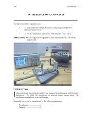
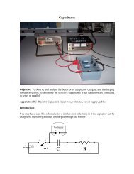
Kinetic energy cutoff “smoothing”
• Existing Abinit strategy to smooth
energy dependence on lattice
parameters in GS calculations
• RF strain derivative calculations
do accurately reproduce GS
numerical derivatives with nonzero
ecutsm
• Divergence can produce large
shifts in elastic tensor if calculation
is not very well converged with
respect to ecut
– Remember, we take two
derivatives
– Perhaps the cutoff function could
be improved
Kinetic energy (Hartree)
100
80
60
40
20
0
ecut = 25
ecutsm = 5
With ecutsm
Without
0 1 2 3 4 5 6 7 8
K (a B -1 )
∞

Strain perturbation for metals
• Thermal smearing of the Fermi surface must be introduced for stability
• In RF calculations, a band of partially-occupied states around ε F is
treated by finite-temperature perturbation theory in the Sternheimer
solution, and only the completely unoccupied states are found by the
conjugate-gradient method (1)
(1)
• For strain, a first-order Fermi energy ε must be introduced (2)
F
(1)
• ε F
enters into the Sternheimer self-consistency process
• Convergence can be rather slow
(1)
ε F
– Only simple mixing is presently used to iterate
– Coupling to the first-order potential iteration through Anderson or CG mixing
may help
(1)
ε F
• Is needed for the Q = 0 interatomic force constant calculations
needed to get the relaxed-atom elastic tensor for metals?
(1) S. de Gironcoli, Phys. Rev. B 51, 6773 (1995)
(2) S. Baroni, S. de Gironcoli, and A. Dal Corso, Rev. Mod. Phys. 73, 515 (2001)

Input file for RF run with strain
# First dataset : Self-consistent run
# Second dataset : Non-self-consistent run
# for full k point set
# Third dataset : d/dk response calculation
#this section is omitted if
getwfk3 2 #only the elastic tensor is
getden3 1 #wanted
iscf3 -3
rfelfd3 2
rfdir3 1 1 1
# Fourth dataset : phonon, strain,and homogeneous
# electric field response
diemix4 0.85
diemac4 1.0
getwfk4 2
getddk4 3 #omitted for ELT only
iscf4 3
rfelfd4 3 #omitted for ELT only
rfatpol4 1 2
rfdir4 1 1 1
rfphon4 1
rfstrs4 3 #only this is new for strain
# Common data #stresses and forces should
nqpt 1 #(in general) be relaxed
qpt 0 0 0 #beforehand

2DTE terms in output file
• Mix of reduced and Cartesian coordinates, also in _DDB output file
– With natom = 2, electric field pert = 4 and strain pert = 5, 6
– Only a sample of the complete matrix shown
2nd-order matrix (non-cartesian coordinates, masses not included,
asr not included )
cartesian coordinates for strain terms (1/ucvol factor
for elastic tensor components not included)
j1 j2 matrix element
dir pert dir pert real part imaginary part
1 1 2 2 -2.8200006186 0.0000000000
1 1 3 2 -2.8654826400 interatomic force constant (red-red)
1 1 1 4 -4.1367712586 Born effective charge (red-red)
1 1 2 5 -0.0238530938 internal strain (red-cart)
1 4 3 4 46.0269881204 dielectric tensor (red-red)
1 4 3 5 -0.2214090328 piezoelectric tensor (red-cart)
1 5 2 6 -0.0103809572 elastic tensor (cart-cart)
• Cartesian ELT, PZT, and internal strain are also included in the output
• Detailed breakdown of contributions is given for prtvol = 10

Incorporating atomic relaxation
• Implemented as post-processing procedure in anaddb
– New and modified routines: dielmore9.f, elast9.f, piezo9.f,
instr9.f, invars9.f, outvars9.f, diel9.f, anaddb.f,
defs_common.f, defs_basis.f
• Full theoretical discussion in Infos/Theory/lr.pdf
• Basic results:
natom 3
−1 −1
αβ, γδ αβγδ , ∑∑ mi, αβ( )
mi, nj nj,
γδ
mn= 1 ij=
1
C!
= C +Ω ΛK
Λ
natom 3
−1 −1
αβ, γ
=
αβ, γ
+Ω ∑∑Λmi, αβ( )
mi, nj nj,
γ
mn= 1 ij=
1
e!
e K Z
CC !,
– physical and clamped-atom elastic tensors
– ee !,
physical and clamped-atom piezoelectric tensors
– K −1 pseudo-inverse Q=0 interatomic force constant matrix
– Λ internal-strain “force response” tensor
– Z Born effective charge matrix
– All in Cartesian coordinates

Input file for anaddb run
dieflag 3
elaflag 3
piezoflag 3
instrflag 1
!flag for relaxed-ion dielectric tensor
!flag for the elastic tensor
!flag for the piezoelectric rensor
!flag for the internal strain tensor
!the effective charge part
asr 1
chneut 1
!Wavevector list number 1
nph1l 1
qph1l 0.0 0.0 0.0 1.0
!Wave vector list no. 2
nph2l 1
qph2l 0.0 0.0 1.0 0.0
New flags and/or values in violet
See Test_v4/t61-70 for more examples

New output from anaddb
Elastic Tensor(relaxed ion)(Unit:10^2GP,VOIGT notation):
1.2499151 0.6699976 0.6835944 0.0022847 -0.0113983 -0.0001512
0.6699976 1.6217899 0.5566207 0.0194005 -0.0055653 -0.0055915
0.6835944 0.5566207 1.5896839 -0.0207927 0.0107924 0.0080825
0.0022847 0.0194005 -0.0207927 0.6659339 0.0077398 -0.0056845
-0.0113983 -0.0055653 0.0107924 0.0077398 0.7283916 0.0014049
-0.0001512 -0.0055915 0.0080825 -0.0056845 0.0014049 0.7222881
proper piezoelectric constants(relaxed ion)(Unit:c/m^2)
0.01714694 0.05107080 -0.00883676
0.00828454 0.03716812 -0.00810176
0.01882065 0.05180658 -0.00576393
-0.03872154 -0.01245206 0.01902693
-0.01424058 0.00757132 -0.00294782
0.01566436 -0.00054740 0.00218470
• Also in output
– Clamped-ion versions of the above in standard units
– Clamped and relaxed compliance tensors
– “Force-response” and “displacement response” internal strain tensors
– More tensors corresponding to different boundary conditions to be added

Global comparison with numerical derivatives
• Zinc-blende AlP with random distortions so all tensor elements are non-zero.
– Ground state calculations of stress and polarization with exquisitely relaxed atomic
coordinates (but unrelaxed stress)
– Finite-difference d/dk ψ (1) α
's for best consistency with polarization calculations
– Sample of complete set of tensor elements
Elastic Tensor (GPa) Piezoelectric Tensor (C/m 2 x 10 -2 )
Numerical DFPT Diff
xx xx 124.991500 124.991500 -1.1E-05
yy xx 66.999750 66.999760 8.2E-06
zz xx 68.359440 68.359440 7.0E-07
yz xx 0.228447 0.228466 1.9E-05
xz xx -1.139838 -1.139828 9.6E-06
xy xx -0.015028 -0.015117 -9.0E-05
xx yz 0.228471 0.228466 -4.4E-06
yy yz 1.940050 1.940054 3.7E-06
zz yz -2.079264 -2.079275 -1.1E-05
yz yz 66.593340 66.593390 5.2E-05
xz yz 0.773972 0.773977 5.1E-06
xy yz -0.568446 -0.568449 -3.2E-06
Numerical DFPT Diff
x xx 1.714769 1.714694 -7.5E-05
y xx 5.107069 5.107080 1.1E-05
z xx -0.883962 -0.883676 2.9E-04
x yy 0.828569 0.828454 -1.2E-04
y yy 3.716843 3.716812 -3.2E-05
z yy -0.810201 -0.810176 2.5E-05
x yz -3.871980 -3.872154 -1.7E-04
y yz -1.245173 -1.245206 -3.3E-05
z yz 1.902687 1.902693 5.6E-06
• RMS Errors 4.0X10 -5 , ELT and 1.7X10 -6 , PZT
– One-two orders of magnitude smaller errors for clamped-atom quantities.

Present status, future development
• Examples of strain RF and anaddb calculations are Test_v4/t61-70
• RF strain is fully parallelized
– Parallel version was developed simultaneously with sequential
• Present limitations
– Norm-conserving psp’s
– Non-spin polarized (this is about to be relaxed, testing is nearly complete)
– LDA only
– No spin-orbit
• GGA prospects
– Probably straightforward but complicated by “two kinds of charge” problem
with model cores
– Model core smoothness problem is undoubtedly worse
• Spin-orbit coupling
– This has all the nonlocal psp complexity, probably significantly worse
judging by the existing spin-orbit code for stress
– Mathematica code will eventually be added to the documentation and may
help a future developer with this

Future development, continued
• PAW
– Far beyond norm-conserving psp non-local complexity
– Needs spherical harmonics with off-diagonal coupling which cannot be
turned into dot products with simple metric-tensor dependencies
– Has “two kinds of charge” problem like model core but much worse,
because augmentation charge has non-spherical components
On the upbeat side, however
• 3 rd -order response functions involving strain via “2n+1” theorem
– Require two y (1) and one H (1) , all available
– Eg., electrostriction, non-linear elastic constants, Grüneisen parameters
• It’s time for feedback – let’s see what the users want and what trouble
they get into
– If a user wants a strain feature badly enough we’ll have a new developer !
– Isn’t that the ABINIT philosophy?
Mat-Sim
Research

Appendix : Mathematica for nonlocal psp
1 i ′⋅ κ
−i
⋅ κ
〈 ′ | VNL
| 〉= ∑
K τ
K τ
K K e fκ
( ′ ⋅ ′) ( ′ ⋅ ′ ′
#
K K℘# K K,K ⋅K,K⋅K) e fκ#
( K⋅K).
Ω
κ#
m
• Define tensor products
T m( K! #
) and T
m( K!
′
#
)
– Follows D. C. Allan
tnk = {
{1}, (* 0, 1 *)
{k1, (* 1, 1 *)
k2, (* 1, 2 *)
k3}, (* 1, 3 *)
{k1 k1, (* 2, 1 *)
k2 k2, (* 2, 2 *)
k3 k3, (* 2, 3 *)
k3 k2, (* 2, 4 *)
etc. to rank 7
• Define K’s, metric tensor
functions, dot products,
and Legengre’s
• s1 and s2 are strain
variables
k = {k1, k2, k3}; kp = {kp1, kp2, kp3};
m = {{m11[s1,s2], m12[s1,s2], m13[s1,s2]},
{m12[s1,s2], m22[s1,s2], m23[s1,s2]},
{m13[s1,s2], m23[s1,s2], m33[s1,s2]}};
dt = kp.m.k; ks = k.m.k; kps = kp.m.kp;
Plegendre={1, dt, 1.5 dt^2 - 0.5 kps ks,
2.5 dt^3 - 1.5 kps dt ks};

Mathematica for nonlocal psp, , continued
• Strain derivatives of form factors “bring out” derivatives of dot products
• Define 6 combinations of dot product derivatives and Legendre
derivatives that have given offsets between “input” and “output” rank
poly = {D[kps,s2] D[kps,s1] Plegendre[[rank+1]],
D[ks, s2] D[ks, s1] Plegendre[[rank+1]],
(D[D[kps,s2],s1] Plegendre[[rank+1]]
+ D[kps,s1] D[Plegendre[[rank+1]],s2]
+ D[kps,s2] D[Plegendre[[rank+1]],s1]),
(D[D[ks, s2],s1] Plegendre[[rank+1]]
+ D[ks, s1] D[Plegendre[[rank+1]],s2]
+ D[ks, s2] D[Plegendre[[rank+1]],s1]),
(D[kps,s1] D[ks,s2] + D[kps,s2] D[ks,s1])
Plegendre[[rank+1]],
D[D[Plegendre[[rank+1]],s2],s1]};
– In Mathematica df/dx is D[f,x]
# → # + 4
# + 4→#
# → # + 2
# + 2→#
# + 2→ # + 2
# →#
• Now, do the work – extract the coefficients of each pair of input and
output tensors
f #
f , f ′′
# #
f ′′,
f
Do[term = Simplify[Coefficient[poly[[iterm]], (tnkp[[rankout+1]][[jj]] *
tnk[[rankin+1]][[ii]])]];
f
# #
,
f
# #
f ′,
f
# #
′
f ′,
f ′
# #
f , f
# #

Title
• X
• X
• X
• X