7. Interference of Sound Waves

2011 Interference - 1 

INTERFERENCE OF SOUND WAVES 

The objectives of this experiment are: 

• To measure the wavelength, frequency, and propagation speed of 

ultrasonic sound waves. 

• To observe interference phenomena with ultrasonic sound waves. 

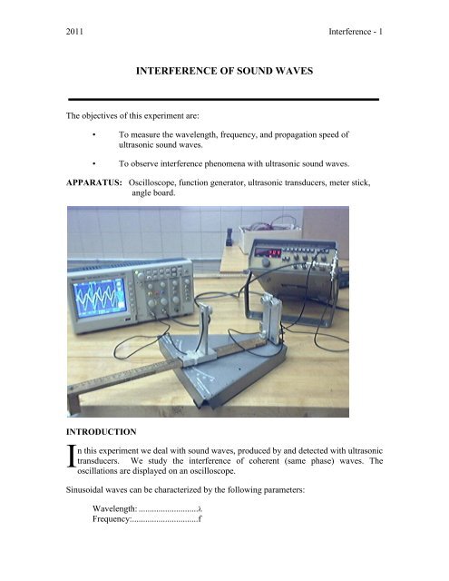
APPARATUS: Oscilloscope, function generator, ultrasonic transducers, meter stick, 

angle board. 

INTRODUCTION 

I 

n this experiment we deal with sound waves, produced by and detected with ultrasonic 

transducers. We study the interference of coherent (same phase) waves. The 

oscillations are displayed on an oscilloscope. 

Sinusoidal waves can be characterized by the following parameters: 

Wavelength: ........................... 

Frequency:..............................f


Period: ....................................T = 1/f 

Wave propagation speed: ......c = f = /T . 

The speed of sound through air (at 20 C) is approximately 344 m/s. 

Ultrasonic transducer 

A transducer is a device that transforms one form of energy into another, for example, a 

microphone (sound to electric) or loudspeaker (electric to sound). In this experiment the 

transducer is a "piezoelectric" crystal of barium titanate which converts electrical 

oscillations into mechanical vibrations that make sound. The oscillating frequency is near 

40 kHz which is beyond what can be heard by the human ear (about 20 kHz). 

Interference of Waves 

Below in Figure 1 is a drawing of the basic concept for interference of coherent waves 

from two point sources. Coherent means that the waves, even though they are from 

separate sources, have the same frequency and are in lock-step, namely in phase, as they 

are being emitted. The waves will get out of relative phase because they have to travel 

different path lengths to reach the same point in space. There, the waves can add 

constructively if they are in phase, or add destructively if they arrive out of phase. Look 

at the diagram. 

FIGURE 1 

S1 and S2 are sound wave sources oscillating in phase because they are driven by the 

same voltage signal generator; they are separated by distance d. The sources also emit 

waves of the same frequency. P is the place where we place a detector, fairly far (in terms


of d) from S1 and S2 . At point P the path difference to S1 and to S2, is the distance 

d sin . When the path difference, d sin is an integral multiple of the wavelength , 

waves arriving at P from S1 and S2 will be in phase and will interfere constructively. 

Note that constructive interference gives maximum intensity: 

d sin 

 

max 

n 

where n = 0, 1, 2,-- is referred to as the order of the particular maximum. 

The Oscilloscope 

We have used FFTscope, a virtual oscilloscope, in previous labs. If you're unfamiliar with 

the basic operation of a real oscilloscope the following should be helpful. Essentially, the 

amplitude of a quantity (usually Voltage) is plotted on the screen as a function of time, in 

real-time. It is possible to display one or two channels (quantities) at the same time; in 

this lab we monitor Driving Voltage from the transmitting transducer (via the function 

generator) and Induced Voltage in the receiving transducers. Here we will monitor the 

receiving transducer on Channel 1 (CH 1, yellow trace) and the transmitting transducers 

on Channel 2 (CH 2, blue trace). 

PROCEDURE: 

1. Learn to use the oscilloscope


1. Position the oscilloscope in front of you. If you wish you can gently flip out the front 

legs so that it is tilted upward for easier viewing. Make sure no cables are plugged into 

the front of the scope for now (T-connectors are okay though). Press the ON button on 

the top left of the scope and wait 35-40 seconds for the grid to show on the display 

(ignore the Language selection screen). If the scope is already on, press the DEFAULT 

SETUP button on the upper-right. 

2. You should see two baseline “noise” traces – Yellow for CH1 and Blue for CH2; this 

is merely background noise since nothing is yet plugged into the scope. 

a. Experiment with adjusting the vertical position of both traces by adjusting the Vertical 

Position knobs above the CH1 Menu and CH2 Menu buttons – this will allow you to 

arrange your plots so that they are not on top of one another. There is also a Horizontal 

Position knob above the SEC/DIV knob. This allows one to move the traces left or right. 

b. Now fiddle with the Sec/Div knob – this sets the size of your time window (horizontal 

axis). If you set the value (look at the “M” value at the bottom-center of the screen) to 

something like 500ms, it'll look like one of those patient monitoring displays at the 

hospital. The M value is the time interval per square. Note that this scope will let you 

examine a time window on the order of a few nanoseconds – an extremely short 

interval of time. 

c. Restore the Sec/Div knob to some intermediate value and now adjust the Volts/Div on 

each channel – this adjusts the gain, or sensitivity of the trace on the vertical axis (i.e. 

potential difference per square). At the highest setting the traces will fluctuate wildly (but 

randomly); at the lowest setting they'll be relatively calm. 

2. Measuring frequency


The setup is shown in Fig. 2 (note that Chnl B in the figure is Ch 2 on the oscilloscope, 

and Chnl A is Ch 1): a variable frequency signal generator drives one ultrasonic 

transducer; its output is also applied to channel 2 (blue trace) of the oscilloscope. (Later 

in the experiment two transmitting transducers will be connected to channel 2.) The 

output of a second receiving ultrasonic generator is applied to channel 1 (yellow trace) of 

the scope. Channel 2 trace (pattern of the oscilloscope) shows the sinusoidal voltage 

applied to the transmitting generator; channel 1 trace shows the sinusoidal voltage 

coming out of the receiving ultrasonic crystal. 

Dual Trace 

Oscilloscope 

Chnl B 

Chnl A 

Function 

Generator 

Receiv er 

Transmitter 

FIGURE 2 

Plug the cables into the appropriate channels as pictured in Figure 2 above. Make sure 

that initially only one of the transmitting transducers is connected to the T-connector. 

Turn on the function generator by pressing the green power button. 

Adjust the scope controls: vertical amplification (Volts/Div), horizontal sweep rate 

(Sec/Div), vertical position, and horizontal position so that trace 1 shows several, steady 

sine curves. Place the transmitting transducer facing the receiver at a distance of a few 

centimeters. If you think the transducers are not functioning (nothing on trace 1), it is 

most likely that the function generator is not at the exact resonance frequency. You 

should tune to resonance when the signal getting through to the receiving transducer 

(trace 1) reaches a maximum. Do this by varrying the frequency around 38 to 42 kHz. Be 

aware that a small red light on the display of the function generator will light up “kHz” if 

the reading is in kHz (as opposed to Hz). This is, of course, what you want. You can see 

that sound signal is being received by placing your hand in front of the transducers. By 

blocking the sound wave, you will disturb or eliminate the yellow trace from Ch 1.


Warning: Do not exchange your transducers with those from other tables; 

your three transducers are a matched set. 

Measure the period of oscillation directly from the oscilloscope's screen, taking into 

account the sweep rate (“M” value at bottom-center of screen). To make the period 

measurement as accurate as possible, measure the time interval corresponding to several 

complete oscillations. That is, measure the total time interval and divide by the total 

number of waves. Use the fine rulings of the square boxes to obtain a precise value. The 

reciprocal of T is f. Compare the frequency fo determined with the oscilloscope with both 

the frequency fsg of the signal generator and the frequency provide by the oscilloscope in 

blue in the lower right corner of the screen. The latter two values will likely be more 

accurate than your computed value, but the point is to gain an understanding of the 

information conveyed by the oscilloscope traces. 

A more precise way to measure the period, which exploits special features of the 

oscilloscope is as follows. Press the Cursor button near the middle of the dozen buttons 

at the top of the face of the scope – this will now change the on-screen Menu on the right 

of the scope screen. The Menu selections can be made by pressing on the buttons 

immediately to the right of the screen; press the button to the right of Type (twice) so that 

the Time cursors are activated. Beneath Type the word “TIME” will appear in a white 

box, and you should now see two vertical lines on the screen. If beneath Source you see 

“Ch 1” or “Ch 2” the vertical lines will be yellow or blue respectively. Either will do 

since both traces pertain to waves of the same frequency and period. However, if you see 

neither “Ch 1” nor “Ch 2” you will need to press the button to the right of Source until 

you are in one of these settings. Turn the knobs labeled VERTICAL Position CURSOR 1 

and CURSOR 2 (i.e. the knobs which usually move the traces the left and right) to move 

the vertical lines left and right. Align one with a wave crest (or trough) to the left of the 

screen and one with a wave crest (or trough) to the right of the screen. Then the read out 

on the right of the screen in blue or yellow will say DELTA beneath which will read the 

time interval between the vertical lines. This information can also be extracted from the 

difference in time values listed for Cursor 2 and Cursor 1 just below DELTA. You need 

only divide by the number of wave cycles in order to determine the period. 

3. Measuring wavelength 

The transmitting and receiving transducer stands fit over, and can slide along, a meter 

stick. With both transducers fixed in position, the two sinusoidal traces on the scope are 

steady. What happens to the scope trace from the receiving transducer when you move 

the receiving transducer away from the transmitting transducer? The traces are providing 

information about the relative phases of the transmitted and received sound wave (or the 

driving voltage and receiver voltage). 

Measure the wavelength by slowly shifting the receiving transducer a known distance 

away from the transmitter while noting on the oscilloscope screen by how many complete 

cycles of relative phase the wave pattern shifts. Don't choose just one cycle, but as many 

cycles as can conveniently be measured along the meter stick.


4. Calculating Speed of Sound 

Use the measured period of ultrasonic oscillations from Part 2 and the wavelength from 

Part 3 to compute the speed of sound through air. Then repeat the calculation using the 

frequency from the signal generator. The oscillation period measured with the scope 

sweep calibration may not be as accurate as the frequency readings on the signal 

generator or oscilloscope display. Compare your computed values with the standard 

value of 344 m/s for dry air at 20 C temperature. Then consider which is more accurate 

and why. 

5. Double Source Interference 

The setup is similar to Fig. 2, but another transmitting transducer is added. This is 

effected by plugging the cable of the second transmitter into the T-connector and 

centering the pair of transmitters on the board (they are attached by a magnet at their 

base, which can slide). The pair of transmitters are placed side-by-side and driven in 

phase by a signal generator; a third receiving transducer is at an angle which can be 

varied. See Fig. 3, which duplicates the arrangement shown in Fig. 1. 

FIGURE 3 

We are interested in observing the amplitude of the resultant ultrasonic wave reaching the 

receiving transducer. When you move the detector you are receiving the combined 

intensity of the two interfering waves. Sometimes you will see a strong signal while other 

times little or none. Move the receiving transducer along a circular arc, maintaining a 

constant distance from the two transmitting transducers. Record the transmitter 

separation d and the angular positions max for interference maxima. The separation 

between transmitters should be kept as small as possible, while the distance of the 

receiver should be as large as possible. However, you may have to compromise on the 

inter-transmitter distance you choose since fewer maxima will be observable for smaller 

distances. For this reason, it may not be possible to see the fourth order maximum. 

Suggestion: rather than plotting max readings directly from the protractor, try taking 

corresponding left-side and right-side values and average them, thus eliminating any error 

in judging where the center line is.


Confirm the constructive interference relation, n = d sinmax, by plotting sin max as a 

function of the integer n. (Take values for n and max on the right side as positive and 

those on the left as negative so your plot is a straight line (sin = -sin) rather than a 

"V"). The slope of your best straight line will enable you to calculate /d, and then the 

wavelength in terms of the measured distance, d, between the transmitters. Compare 

this with the value of measured in part 4. Obviously the slope will also give you d/. 

Thus you can find the separation d in terms of the theoretical wavelength = c/f. 

Compare this with the value of d directly measured.


INTERFERENCE OF SOUND WAVES 

LAB REPORT FORM 

Name:___________________________________________________ Section:________ 

Partner: _____________________________________________________Date: _______ 

2) Frequency Measurement 

Oscilloscope Time Base Per Div (TB): __________ 

Number of Waves Counted on Screen (NW):_________ 

Number (& fractional parts) of Divisions Covered by Waves (ND): ________ 

Period of One Wave = TB * ND / NW = _________ Frequency = _________ 

Frequency from signal generator, = __________ 

Frequency from oscilloscope display = __________ 

3) Wavelength Measurement 

Number of Waves Moved on Oscilloscope Nw: _________ 

Initial Position of Movable Sensor Pi: __________ 

Final Position of Movable Sensor Pf: ___________ 

Distance sensor moved, Pi - Pf = D: _____________ 

Length of One Wave, Wavelength = D/Nw : ___________ 

What happens to the scope trace from the receiving transducer when you move the 

receiving transducer away from the transmitting transducer? How does this allow you to 

calculate wavelength? Explain. 

4) Speed of Sound: Use your wavelength and frequency (as determined with 

oscilloscope) to calculate c. Do the same with the function generator frequency. 

c = = _____________ c = =_____________ 

Compare your computed values with the standard value of 344 m/s for dry air at 20 C 

temperature. Which is better?


5) Interference of Sound Separation of Sources, d: _________ 

max sin(max) n (maximum #) 

Graph sin(max) vs. n. Measure slope of line fitted to data. 

slope = /d = ______ (recall, n = d sinmax) 

use measured d to get _____ 

Compare wavelength measured on the oscilloscope (Part 3) with the value from 

interference (Part 5): 

R (ratio) = oscint = __________ 

The slope of your best straight line also enables you to calculate (d/), and thus the 

separation d in terms of the theoretical wavelength = c/f. Use the theoretical value of c 

and the value of frequency which gave the most accurate speed in part 4 to compute 

lambda. Compare this with the value of d directly measured.

7. Interference of Sound Waves

You also want an ePaper? Increase the reach of your titles

Delete template?

Save as template?