26. passage of particles through matter - Particle Data Group
26. passage of particles through matter - Particle Data Group
26. passage of particles through matter - Particle Data Group

You also want an ePaper? Increase the reach of your titles
YUMPU automatically turns print PDFs into web optimized ePapers that Google loves.
<strong>26.</strong> Passage <strong>of</strong> <strong>particles</strong> <strong>through</strong> <strong>matter</strong> 1<br />
<strong>26.</strong> PASSAGE OF PARTICLES THROUGH MATTER<br />
Revised April 2002 by H. Bichsel (University <strong>of</strong> Washington), D.E. Groom (LBNL), and<br />
S.R. Klein (LBNL).<br />
<strong>26.</strong>1. Notation<br />
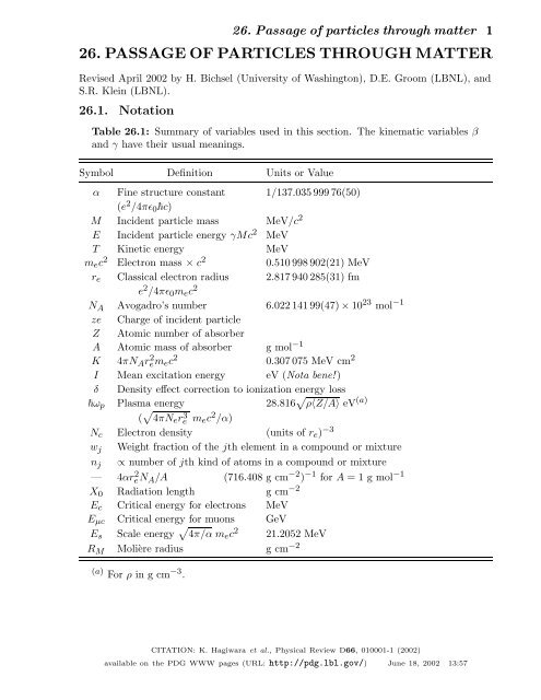
Table <strong>26.</strong>1: Summary <strong>of</strong> variables used in this section. The kinematic variables β<br />
and γ have their usual meanings.<br />
Symbol Definition Units or Value<br />
α Fine structure constant 1/137.035 999 76(50)<br />
(e 2 /4πɛ 0 ~c)<br />
M Incident particle mass MeV/c 2<br />
E Incident particle energy γMc 2 MeV<br />
T Kinetic energy MeV<br />
m e c 2 Electron mass × c 2 0.510 998 902(21) MeV<br />
r e Classical electron radius 2.817 940 285(31) fm<br />
e 2 /4πɛ 0 m e c 2<br />
N A Avogadro’s number 6.022 141 99(47) × 10 23 mol −1<br />
ze Charge <strong>of</strong> incident particle<br />
Z Atomic number <strong>of</strong> absorber<br />
A Atomic mass <strong>of</strong> absorber g mol −1<br />
K 4πN A rem 2 e c 2 0.307 075 MeV cm 2<br />
I Mean excitation energy eV (Nota bene! )<br />
δ Density effect correction to ionization energy loss<br />
~ω p Plasma energy 28.816 √ ρ〈Z/A〉 eV (a)<br />
( √ 4πN e re 3 m ec 2 /α)<br />
N c Electron density (units <strong>of</strong> r e ) −3<br />
w j Weight fraction <strong>of</strong> the jth element in a compound or mixture<br />
n j ∝ number <strong>of</strong> jth kind <strong>of</strong> atoms in a compound or mixture<br />
— 4αre 2N A/A (716.408 g cm −2 ) −1 for A =1gmol −1<br />
X 0 Radiation length g cm −2<br />
E c Critical energy for electrons MeV<br />
E µc Critical energy for muons GeV<br />
E s Scale energy √ 4π/α m e c 2 21.2052 MeV<br />
R M Molière radius g cm −2<br />
(a) For ρ in g cm −3 .<br />
CITATION: K. Hagiwara et al., Physical Review D66, 010001-1 (2002)<br />
available on the PDG WWW pages (URL: http://pdg.lbl.gov/) June 18, 2002 13:57
2 <strong>26.</strong> Passage <strong>of</strong> <strong>particles</strong> <strong>through</strong> <strong>matter</strong><br />
<strong>26.</strong>2. Electronic energy loss by heavy <strong>particles</strong> [1–5]<br />
Moderately relativistic charged <strong>particles</strong> other than electrons lose energy in <strong>matter</strong><br />
primarily by ionization and atomic excitation. The mean rate <strong>of</strong> energy loss (or stopping<br />
power) is given by the Bethe-Bloch equation,<br />
− dE<br />
[<br />
dx = Kz2Z 1 1<br />
A β 2 2 ln 2m ec 2 β 2 γ 2 T max<br />
I 2 − β 2 − δ ]<br />
. (<strong>26.</strong>1)<br />
2<br />
Here T max is the maximum kinetic energy which can be imparted to a free electron in a<br />
single collision, and the other variables are defined in Table <strong>26.</strong>1. With K as defined in<br />
Table <strong>26.</strong>1 and A in g mol −1 , the units are MeV g −1 cm 2 .<br />
In this form, the Bethe-Bloch equation describes the energy loss <strong>of</strong> pions in a material<br />
such as copper to about 1% accuracy for energies between about 6 MeV and 6 GeV<br />
Stopping power [MeV cm 2 /g]<br />
100<br />
10<br />
1<br />
Lindhard-<br />
Scharff<br />
Nuclear<br />
losses<br />
µ −<br />
Anderson-<br />
Ziegler<br />
Bethe-Bloch<br />
Minimum<br />
ionization<br />
µ + on Cu<br />
Radiative<br />
effects<br />
reach 1%<br />
Radiative<br />
Radiative<br />
losses<br />
Without δ<br />
0.001 0.01 0.1 1 10 100 1000 10 4 10 5 10 6<br />
βγ<br />
0.1 1 10 100 1 10 100 1 10 100<br />
[MeV/c]<br />
[GeV/c]<br />
[TeV/c]<br />
Muon momentum<br />
E µc<br />
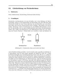
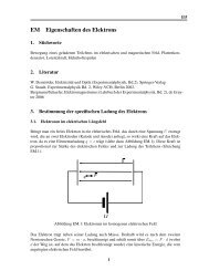
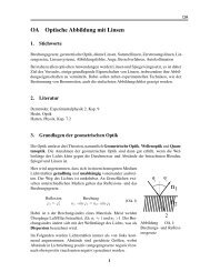
Fig. <strong>26.</strong>1: Stopping power (= 〈−dE/dx〉) for positive muons in copper<br />
as a function <strong>of</strong> βγ = p/Mc over nine orders <strong>of</strong> magnitude in momentum<br />
(12 orders <strong>of</strong> magnitude in kinetic energy). Solid curves indicate the<br />
total stopping power. <strong>Data</strong> below the break at βγ ≈ 0.1 are taken from<br />
ICRU 49 [2], and data at higher energies are from Ref. 1. Vertical bands<br />
indicate boundaries between different approximations discussed in the text.<br />
The short dotted lines labeled “µ − ” illustrate the “Barkas effect,” the<br />
dependence <strong>of</strong> stopping power on projectile charge at very low energies [6].<br />
June 18, 2002 13:57
<strong>26.</strong> Passage <strong>of</strong> <strong>particles</strong> <strong>through</strong> <strong>matter</strong> 3<br />
(momenta between about 40 MeV/c and 6 GeV/c). At lower energies various corrections<br />
discussed in Sec. <strong>26.</strong>2.1 must be made. At higher energies, radiative effects begin to be<br />
important. These limits <strong>of</strong> validity depend on both the effective atomic number <strong>of</strong> the<br />
absorber and the mass <strong>of</strong> the slowing particle.<br />
The function as computed for muons on copper is shown by the solid curve in Fig. <strong>26.</strong>1,<br />
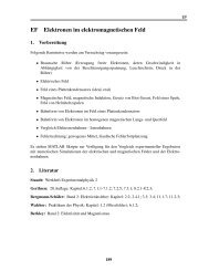
and for pions on other materials in Fig. <strong>26.</strong>3. A minor dependence on M at the highest<br />
energies is introduced <strong>through</strong> T max , but for all practical purposes in high-energy physics<br />
dE/dx in a given material is a function only <strong>of</strong> β. Except in hydrogen, <strong>particles</strong> <strong>of</strong><br />
the same velocity have similar rates <strong>of</strong> energy loss in different materials; there is a<br />
slow decrease in the rate <strong>of</strong> energy loss with increasing Z. The qualitative difference in<br />
stopping power behavior at high energies between a gas (He) and the other materials<br />
shown in Fig. <strong>26.</strong>3 is due to the density-effect correction, δ, discussed below. The stopping<br />
power functions are characterized by broad minima whose position drops from βγ =3.5<br />
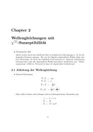
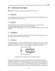
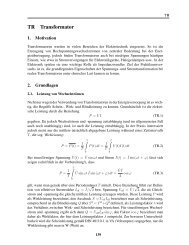
to 3.0 as Z goes from 7 to 100. The values <strong>of</strong> minimum ionization as a function <strong>of</strong> atomic<br />
number are shown in Fig. <strong>26.</strong>2.<br />
In practical cases, most relativistic <strong>particles</strong> (e.g., cosmic-ray muons) have mean energy<br />
loss rates close to the minimum, and are said to be minimum ionizing <strong>particles</strong>, or mip’s.<br />
As discussed below, the most probable energy loss in a detector is considerably below<br />
the mean given by the Bethe-Bloch equation.<br />
〈–dE/dx〉 min (MeV g –1 cm 2 )<br />
2.5<br />
2.0<br />
1.5<br />
1.0<br />
H 2 gas: 4.10<br />
H 2 liquid: 3.97<br />
Solids<br />
Gases<br />
2.35 – 1.47 ln(Z)<br />
0.5<br />
H He Li Be B CNONe Fe Sn<br />
1 2 5 10 20 50 100<br />
Z<br />
Figure <strong>26.</strong>2: Stopping power at minimum ionization for the chemical elements.<br />
ThestraightlineisfittedforZ>6. A simple functional dependence on Z is not to<br />
be expected, since 〈−dE/dx〉 also depends on other variables.<br />
Eq. (<strong>26.</strong>1) may be integrated to find the total (or partial) “continuous slowing-down<br />
approximation” (CSDA) range R for a particle which loses energy only <strong>through</strong> ionization<br />
June 18, 2002 13:57
4 <strong>26.</strong> Passage <strong>of</strong> <strong>particles</strong> <strong>through</strong> <strong>matter</strong><br />
10<br />
8<br />
− dE/dx (MeV g −1 cm 2 )<br />
6<br />
5<br />
4<br />
3<br />
2<br />
H 2 liquid<br />
He gas<br />
Fe<br />
Sn<br />
Pb<br />
Al<br />
C<br />
1<br />
0.1<br />
1.0 10 100 1000 10 000<br />
βγ = p/Mc<br />
0.1<br />
0.1<br />
1.0 10 100 1000<br />
Muon momentum (GeV/c)<br />
1.0 10 100 1000<br />
Pion momentum (GeV/c)<br />
0.1<br />
1.0 10 100 1000 10 000<br />
Proton momentum (GeV/c)<br />
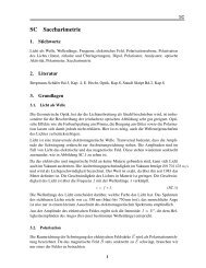
Figure <strong>26.</strong>3: Mean energy loss rate in liquid (bubble chamber) hydrogen, gaseous<br />
helium, carbon, aluminum, iron, tin, and lead. Radiative effects, relevant for<br />
muons and pions, are not included. These become significant for muons in iron for<br />
βγ > ∼ 1000, and at lower momenta for muons in higher-Z absorbers. See Fig. <strong>26.</strong>20.<br />
and atomic excitation. Since dE/dx depends only on β, R/M is a function <strong>of</strong> E/M or<br />
pc/M. In practice, range is a useful concept only for low-energy hadrons (R < ∼ λ I ,where<br />
λ I is the nuclear interaction length), and for muons below a few hundred GeV (above<br />
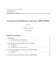
which radiative effects dominate). R/M as a function <strong>of</strong> βγ = p/Mc is shown for a<br />
variety <strong>of</strong> materials in Fig. <strong>26.</strong>4.<br />
The mass scaling <strong>of</strong> dE/dx and range is valid for the electronic losses described by the<br />
Bethe-Bloch equation, but not for radiative losses, relevant only for muons and pions.<br />
For a particle with mass M and momentum Mβγc, T max is given by<br />
T max =<br />
2m e c 2 β 2 γ 2<br />
1+2γm e /M +(m e /M ) 2 . (<strong>26.</strong>2)<br />
June 18, 2002 13:57
<strong>26.</strong> Passage <strong>of</strong> <strong>particles</strong> <strong>through</strong> <strong>matter</strong> 5<br />
50000<br />
20000<br />
10000<br />
5000<br />
Pb<br />
Fe<br />
C<br />
R/M (g cm −2 GeV −1 )<br />
2000<br />
1000<br />
500<br />
200<br />
100<br />
50<br />
20<br />
10<br />
5<br />
H 2 liquid<br />
He gas<br />
2<br />
1<br />
0.1 2 5 1.0 2 5 10.0 2 5 100.0<br />
βγ = p/Mc<br />
0.02 0.05 0.1 0.2 0.5 1.0 2.0 5.0 10.0<br />
Muon momentum (GeV/c)<br />
0.02 0.05 0.1 0.2 0.5 1.0 2.0 5.0 10.0<br />
Pion momentum (GeV/c)<br />
0.1 0.2 0.5 1.0 2.0 5.0 10.0 20.0 50.0<br />
Proton momentum (GeV/c)<br />
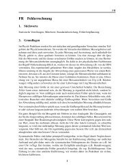
Figure <strong>26.</strong>4: Range <strong>of</strong> heavy charged <strong>particles</strong> in liquid (bubble chamber)<br />
hydrogen, helium gas, carbon, iron, and lead. For example: For a K + whose<br />
momentum is 700 MeV/c, βγ =1.42. For lead we read R/M ≈ 396, and so the<br />
rangeis195gcm −2 .<br />
In older references [3,4] the “low-energy” approximation<br />
T max =2m e c 2 β 2 γ 2 , valid for 2γm e /M ≪ 1, is <strong>of</strong>ten implicit. For a pion in copper, the<br />
error thus introduced into dE/dx is greater than 6% at 100 GeV. The correct expression<br />
should be used.<br />
At energies <strong>of</strong> order 100 GeV, the maximum 4-momentum transfer to the electron can<br />
exceed 1 GeV/c, where hadronic structure effects significantly modify the cross sections.<br />
This problem has been investigated by J.D. Jackson [7], who concluded that for hadrons<br />
(but not for large nuclei) corrections to dE/dx are negligible below energies where<br />
June 18, 2002 13:57
6 <strong>26.</strong> Passage <strong>of</strong> <strong>particles</strong> <strong>through</strong> <strong>matter</strong><br />
radiative effects dominate. While the cross section for rare hard collisions is modified, the<br />
average stopping power, dominated by many s<strong>of</strong>ter collisions, is almost unchanged.<br />
“The determination <strong>of</strong> the mean excitation energy is the principal non-trivial task in<br />
the evaluation <strong>of</strong> the Bethe stopping-power formula” [8]. Recommended values have varied<br />
substantially with time. Estimates based on experimental stopping-power measurements<br />
for protons, deuterons, and alpha <strong>particles</strong> and on oscillator-strength distributions and<br />
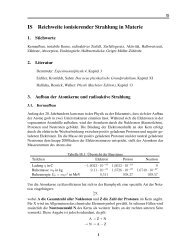
dielectric-response functions were given in ICRU 37 [9]. These values, shown in Fig. <strong>26.</strong>5,<br />
have since been widely used. Machine-readable versions can also be found [10]. These<br />
values are widely used.<br />
22<br />
20<br />
I adj /Z (eV)<br />
18<br />
16<br />
14<br />
12<br />
10<br />
ICRU 37 (1984)<br />
(interpolated values are<br />
not marked with points)<br />
Barkas & Berger 1964<br />
Bichsel 1992<br />
8<br />
0 10 20 30 40 50 60 70 80 90 100<br />
Z<br />
Figure <strong>26.</strong>5: Mean excitation energies (divided by Z) as adopted by the ICRU [9].<br />
Those based on experimental measurements are shown by symbols with error flags;<br />
the interpolated values are simply joined. The grey point is for liquid H 2 ; the black<br />
point at 19.2 eV is for H 2 gas. The open circles show more recent determinations by<br />
Bichsel [11]. The dotted curve is from the approximate formula <strong>of</strong> Barkas [12] used<br />
in early editions <strong>of</strong> this Review.<br />
<strong>26.</strong>2.1. Energy loss at low energies: Shell corrections C/Z must be included in the<br />
square brackets <strong>of</strong> <strong>of</strong> Eq. (<strong>26.</strong>1) [2,9,11,12] to correct for atomic binding having been<br />
neglected in calculating some <strong>of</strong> the contributions to Eq. (<strong>26.</strong>1). The Barkas form [12]<br />
was used in generating Fig. <strong>26.</strong>1. For copper it contributes about 1% at βγ =0.3 (kinetic<br />
energy 6 MeV for a pion), and the correction decreases very rapidly with energy.<br />
Eq. (<strong>26.</strong>1) is based on a first-order Born approximation. Higher-order corrections,<br />
again important only at lower energy, are normally included by adding a term z 2 L 2 (β)<br />
inside the square brackets.<br />
June 18, 2002 13:57
<strong>26.</strong> Passage <strong>of</strong> <strong>particles</strong> <strong>through</strong> <strong>matter</strong> 7<br />
An additional “Barkas correction” zL 1 (β) makes the stopping power for a negative<br />
particle somewhat larger than for a positive particle with the same mass and velocity. In<br />
a 1956 paper, Barkas et al. noted that negative pions had a longer range than positive<br />
pions [6]. The effect has been measured for a number <strong>of</strong> negative/positive particle pairs,<br />
most recently for antiprotons at the CERN LEAR facility [13].<br />
A detailed discussion <strong>of</strong> low-energy corrections to the Bethe formula is given in<br />
ICRU Report 49 [2]. When the corrections are properly included, the accuracy <strong>of</strong> the<br />
Bethe-Bloch treatment is accurate to about 1% down to β ≈ 0.05, or about 1 MeV for<br />
protons.<br />
For 0.01
8 <strong>26.</strong> Passage <strong>of</strong> <strong>particles</strong> <strong>through</strong> <strong>matter</strong><br />
mixtures <strong>of</strong> interest are published in a variety <strong>of</strong> places, notably in Ref. 21. A recipe for<br />
finding the coefficients for nontabulated materials is given by Sternheimer and Peierls [19],<br />
and is summarized in Ref. 1.<br />
The remaining relativistic rise comes from the β 2 γ 2 growth <strong>of</strong> T max , which in turn is<br />
due to (rare) large energy transfers to a few electrons, to be discussed below. When these<br />
events are excluded, the energy deposit in an absorbing layer approaches a constant value,<br />
the Fermi plateau (see Sec. <strong>26.</strong>2.4 below). At extreme energies (e.g., > 332 GeV for<br />
muons in iron, and at a considerably higher energy for protons in iron), radiative effects<br />
are more important than ionization losses. These are especially relevant for high-energy<br />
muons, as discussed in Sec. <strong>26.</strong>6.<br />
<strong>26.</strong>2.3. Energetic knock-on electrons (δ rays): The distribution <strong>of</strong> secondary<br />
electrons with kinetic energies T ≫ I is given by [3]<br />
d 2 N<br />
dT dx = 1 2 Kz2Z A<br />
1 F(T)<br />
β 2 T 2 (<strong>26.</strong>5)<br />
for I ≪ T ≤ T max ,whereT max is given by Eq. (<strong>26.</strong>2). Here β is the velocity <strong>of</strong> the<br />
primary particle. The factor F is spin-dependent, but is about unity for T ≪ T max . For<br />
spin-0 <strong>particles</strong> F (T )=(1−β 2 T/T max ); forms for spins 1/2 and 1 are also given by<br />
Rossi [3]. For incident electrons, the indistinguishability <strong>of</strong> projectile and target means<br />
that the range <strong>of</strong> T extends only to half the kinetic energy <strong>of</strong> the incident particle.<br />
Additional formulae are given in Ref. 22. Equation (<strong>26.</strong>5) is inaccurate for T close to<br />
I: for 2I < ∼ T < ∼ 10I, the1/T 2 dependence above becomes approximately T −η ,with<br />
3< ∼ η< ∼ 5 [23].<br />
δ rays <strong>of</strong> appreciable energy are rare. For example, for a 500 MeV pion incident on a<br />
silicon detector with thickness x = 300 µm, one may integrate Eq. (<strong>26.</strong>5) from T cut to<br />
T max to find that x(dN/dx) = 1, or an average <strong>of</strong> one δ ray per particle crossing, for T cut<br />
equal to only 12 keV. For T cut = 116 keV (the mean minimum energy loss in 300 µm <strong>of</strong><br />
silicon), x(dN/dx) =0.0475—less than one particle in 20 produces a δ ray with kinetic<br />
energy greater than T cut . ∗<br />
A δ ray with kinetic energy T e and corresponding momentum p e is produced at an<br />
angle θ given by<br />
cos θ =(T e /p e )(p max /T max ) , (<strong>26.</strong>6)<br />
where p max is the momentum <strong>of</strong> an electron with the maximum possible energy transfer<br />
T max .<br />
∗ These calculations assume a spin-0 incident particle and the validity <strong>of</strong> the Rutherford<br />
cross section used in Eq. (<strong>26.</strong>5).<br />
June 18, 2002 13:57
<strong>26.</strong> Passage <strong>of</strong> <strong>particles</strong> <strong>through</strong> <strong>matter</strong> 9<br />
<strong>26.</strong>2.4. Restricted energy loss rates for relativistic ionizing <strong>particles</strong>: Further<br />
insight can be obtained by examining the mean energy deposit by an ionizing particle<br />
when energy transfers are restricted to T ≤ T cut ≤ T max . The restricted energy loss rate<br />
is<br />
− dE<br />
dx ∣ = Kz 2Z [<br />
1 1<br />
T
10 <strong>26.</strong> Passage <strong>of</strong> <strong>particles</strong> <strong>through</strong> <strong>matter</strong><br />
∆/x (MeV g −1 cm 2 )<br />
0.50 1.00 1.50 2.00 2.50<br />
f (∆/x)<br />
1.0<br />
0.8<br />
0.6<br />
0.4<br />
0.2<br />
w<br />
500 MeV pion in silicon<br />
640 µm (149 mg/cm 2 )<br />
320 µm (74.7 mg/cm 2 )<br />
160 µm (37.4 mg/cm 2 )<br />
80 µm (18.7 mg/cm 2 )<br />
Mean energy<br />
loss rate<br />
0.0<br />
100 200 300 400 500 600<br />
∆/x (eV/µm)<br />
Figure <strong>26.</strong>6: Straggling functions in silicon for 500 MeV pions, normalized to unity<br />
at the most probable value ∆ p /x. The width w is the full width at half maximum.<br />
1.00<br />
0.95<br />
0.90<br />
(∆p/x) / dE/dxmin<br />
0.85<br />
0.80<br />
0.75<br />
0.70<br />
0.65<br />
0.60<br />
x = 640 µm (149 mg/cm 2 )<br />
320 µm (74.7 mg/cm 2 )<br />
160 µm (37.4 mg/cm 2 )<br />
80 µm (18.7 mg/cm 2 )<br />
0.55<br />
0.50<br />
0.3 1 3 10 30 100 300 1000<br />
βγ (= p/m)<br />
Figure <strong>26.</strong>7: Most probable energy loss in silicon, scaled to the mean loss <strong>of</strong> a<br />
minimum ionizing particle, 388 eV/µm (1.66 MeV g −1 cm 2 ).<br />
June 18, 2002 13:57
<strong>26.</strong> Passage <strong>of</strong> <strong>particles</strong> <strong>through</strong> <strong>matter</strong> 11<br />
<strong>26.</strong>2.6. Energy loss in mixtures and compounds: A mixture or compound can be<br />
thought <strong>of</strong> as made up <strong>of</strong> thin layers <strong>of</strong> pure elements in the right proportion (Bragg<br />
additivity). In this case,<br />
dE<br />
dx = ∑ w j<br />
dE<br />
dx<br />
∣ , (<strong>26.</strong>8)<br />
j<br />
where dE/dx| j isthemeanrate<strong>of</strong>energyloss(inMeVgcm −2 )inthejth element.<br />
Eq. (<strong>26.</strong>1) can be inserted into Eq. (<strong>26.</strong>8) to find expressions for 〈Z/A〉, 〈I 〉, and〈δ〉;<br />
for example, 〈Z/A〉 = ∑ w j Z j /A j = ∑ n j Z j / ∑ n j A j . However, 〈I 〉 as defined this way<br />
is an underestimate, because in a compound electrons are more tightly bound than in<br />
the free elements, and 〈δ〉 as calculated this way has little relevance, because it is the<br />
electron density which <strong>matter</strong>s. If possible, one uses the tables given in Refs. 21 and 28,<br />
which include effective excitation energies and interpolation coefficients for calculating<br />
the density effect correction for the chemical elements and nearly 200 mixtures and<br />
compounds. If a compound or mixture is not found, then one uses the recipe for δ given<br />
in Ref. 19 (repeated in Ref. 1), and calculates 〈I〉 according to the discussion in Ref. 8.<br />
(Note the “13%” rule!)<br />
<strong>26.</strong>2.7. Ionization yields: Physicists frequently relate total energy loss to the number<br />
<strong>of</strong> ion pairs produced near the particle’s track. This relation becomes complicated for<br />
relativistic <strong>particles</strong> due to the wandering <strong>of</strong> energetic knock-on electrons whose ranges<br />
exceed the dimensions <strong>of</strong> the fiducial volume. For a qualitative appraisal <strong>of</strong> the nonlocality<br />
<strong>of</strong> energy deposition in various media by such modestly energetic knock-on electrons,<br />
see Ref. 29. The mean local energy dissipation per local ion pair produced, W , while<br />
essentially constant for relativistic <strong>particles</strong>, increases at slow particle speeds [30]. For<br />
gases, W can be surprisingly sensitive to trace amounts <strong>of</strong> various contaminants [30].<br />
Furthermore, ionization yields in practical cases may be greatly influenced by such factors<br />
as subsequent recombination [31].<br />
<strong>26.</strong>3. Multiple scattering <strong>through</strong> small angles<br />
A charged particle traversing a medium is deflected by many small-angle scatters.<br />
Most <strong>of</strong> this deflection is due to Coulomb scattering from nuclei, and hence the effect<br />
is called multiple Coulomb scattering. (However, for hadronic projectiles, the strong<br />
interactions also contribute to multiple scattering.) The Coulomb scattering distribution<br />
is well represented by the theory <strong>of</strong> Molière [32]. It is roughly Gaussian for small<br />
deflection angles, but at larger angles (greater than a few θ 0 , defined below) it behaves<br />
like Rutherford scattering, having larger tails than does a Gaussian distribution.<br />
If we define<br />
θ 0 = θ rms<br />
plane =<br />
1 √<br />
2<br />
θ rms<br />
space . (<strong>26.</strong>9)<br />
then it is sufficient for many applications to use a Gaussian approximation for the central<br />
98% <strong>of</strong> the projected angular distribution, with a width given by [33,34]<br />
13.6 MeV<br />
θ 0 = z √ ]<br />
x/X 0<br />
[1+0.038 ln(x/X 0 ) . (<strong>26.</strong>10)<br />
βcp<br />
June 18, 2002 13:57
12 <strong>26.</strong> Passage <strong>of</strong> <strong>particles</strong> <strong>through</strong> <strong>matter</strong><br />
Here p, βc, andzare the momentum, velocity, and charge number <strong>of</strong> the incident particle,<br />
and x/X 0 is the thickness <strong>of</strong> the scattering medium in radiation lengths (defined below).<br />
This value <strong>of</strong> θ 0 isfromafittoMolière distribution [32] for singly charged <strong>particles</strong> with<br />
β =1forallZ, and is accurate to 11% or better for 10 −3
<strong>26.</strong> Passage <strong>of</strong> <strong>particles</strong> <strong>through</strong> <strong>matter</strong> 13<br />
Figure <strong>26.</strong>8 shows these and other quantities sometimes used to describe multiple<br />
Coulomb scattering. They are<br />
ψ rms<br />
plane = √ 1 θ rms<br />
3<br />
plane = √ 1 θ 0 , (<strong>26.</strong>13)<br />
3<br />
y rms<br />
plane =<br />
1 √<br />
3<br />
xθ rms<br />
plane = 1 √<br />
3<br />
xθ 0 , (<strong>26.</strong>14)<br />
s plane rms = 1<br />
4 √ 3 xθrms plane = 1<br />
4 √ 3 xθ 0 . (<strong>26.</strong>15)<br />
All the quantitative estimates in this section apply only in the limit <strong>of</strong> small θ rms<br />
plane<br />
and in the absence <strong>of</strong> large-angle scatters. The random variables s, ψ, y, andθin a<br />
given plane are distributed in a correlated fashion (see Sec. 30.1 <strong>of</strong> this Review for the<br />
definition <strong>of</strong> the correlation coefficient). Obviously, y ≈ xψ. In addition, y and θ have<br />
the correlation coefficient ρ yθ = √ 3/2 ≈ 0.87. For Monte Carlo generation <strong>of</strong> a joint<br />
(y plane ,θ plane ) distribution, or for other calculations, it may be most convenient to work<br />
with independent Gaussian random variables (z 1 ,z 2 ) with mean zero and variance one,<br />
andthenset<br />
y plane =z 1 xθ 0 (1 − ρ 2 yθ )1/2 / √ 3+z 2 ρ yθ xθ 0 / √ 3<br />
=z 1 xθ 0 / √ 12 + z 2 xθ 0 /2; (<strong>26.</strong>16)<br />
θ plane =z 2 θ 0 . (<strong>26.</strong>17)<br />
Note that the second term for y plane equals xθ plane /2 and represents the displacement<br />
that would have occurred had the deflection θ plane all occurred at the single point x/2.<br />
For heavy ions the multiple Coulomb scattering has been measured and compared with<br />
various theoretical distributions [35].<br />
<strong>26.</strong>4. Photon and electron interactions in <strong>matter</strong><br />
<strong>26.</strong>4.1. Radiation length: High-energy electrons predominantly lose energy in <strong>matter</strong><br />
by bremsstrahlung, and high-energy photons by e + e − pair production. The characteristic<br />
amount <strong>of</strong> <strong>matter</strong> traversed for these related interactions is called the radiation length X 0 ,<br />
usually measured in g cm −2 . It is both (a) the mean distance over which a high-energy<br />
electron loses all but 1/e <strong>of</strong> its energy by bremsstrahlung, and (b) 7 9<br />
<strong>of</strong> the mean free<br />
path for pair production by a high-energy photon [36]. It is also the appropriate scale<br />
length for describing high-energy electromagnetic cascades. X 0 has been calculated and<br />
tabulated by Y.S. Tsai [37]:<br />
1<br />
X 0<br />
=4αr 2 e<br />
N<br />
{ A<br />
Z 2[ L<br />
A rad − f(Z) ] }<br />
+ ZL ′ rad . (<strong>26.</strong>18)<br />
For A =1gmol −1 , 4αre 2N A/A = (716.408 g cm −2 ) −1 . L rad and L ′ rad<br />
are given in<br />
Table <strong>26.</strong>2. The function f(Z) is an infinite sum, but for elements up to uranium can be<br />
represented to 4-place accuracy by<br />
f(Z) =a 2[ (1 + a 2 ) −1 +0.20206<br />
−0.0369 a 2 +0.0083 a 4 − 0.002 a 6] , (<strong>26.</strong>19)<br />
June 18, 2002 13:57
14 <strong>26.</strong> Passage <strong>of</strong> <strong>particles</strong> <strong>through</strong> <strong>matter</strong><br />
where a = αZ [38].<br />
Table <strong>26.</strong>2: Tsai’s L rad and L ′ rad<br />
, for use in calculating the radiation length in an<br />
element using Eq. (<strong>26.</strong>18).<br />
Element Z L rad L ′ rad<br />
H 1 5.31 6.144<br />
He 2 4.79 5.621<br />
Li 3 4.74 5.805<br />
Be 4 4.71 5.924<br />
Others > 4 ln(184.15 Z −1/3 ) ln(1194 Z −2/3 )<br />
Although it is easy to use Eq. (<strong>26.</strong>18) to calculate X 0 , the functional dependence on Z<br />
is somewhat hidden. Dahl provides a compact fit to the data [39]:<br />
716.4 g cm −2 A<br />
X 0 =<br />
Z(Z + 1) ln(287/ √ (<strong>26.</strong>20)<br />
Z)<br />
Results obtained with this formula agree with Tsai’s values to better than 2.5% for all<br />
elements except helium, where the result is about 5% low.<br />
(X 0 N A /A) ydσ LPM /dy<br />
1.2<br />
0.8<br />
0.4<br />
0<br />
100 GeV<br />
10 GeV<br />
1 TeV<br />
10 TeV<br />
100 TeV<br />
Bremsstrahlung<br />
1 PeV<br />
10 PeV<br />
0 0.25 0.5 0.75 1<br />
y = k/E<br />
Figure <strong>26.</strong>10: The normalized bremsstrahlung cross section kdσ LP M /dk in lead<br />
versus the fractional photon energy y = k/E. The vertical axis has units <strong>of</strong> photons<br />
per radiation length.<br />
The radiation length in a mixture or compound may be approximated by<br />
1/X 0 = ∑ w j /X j , (<strong>26.</strong>21)<br />
where w j and X j are the fraction by weight and the radiation length for the jth element.<br />
June 18, 2002 13:57
<strong>26.</strong> Passage <strong>of</strong> <strong>particles</strong> <strong>through</strong> <strong>matter</strong> 15<br />
Positrons<br />
Lead (Z = 82)<br />
0.20<br />
− 1 dE (X −1<br />
E dx 0 )<br />
1.0<br />
0.5<br />
Electrons<br />
Ionization<br />
Møller (e − )<br />
Bhabha (e + )<br />
Bremsstrahlung<br />
0.15<br />
0.10<br />
(cm 2 g −1 )<br />
0.05<br />
0<br />
1<br />
Positron<br />
annihilation<br />
10 100 1000<br />
E (MeV)<br />
Figure <strong>26.</strong>9: Fractional energy loss per radiation length in lead as a function <strong>of</strong><br />
electron or positron energy. Electron (positron) scattering is considered as ionization<br />
when the energy loss per collision is below 0.255 MeV, and as Moller (Bhabha)<br />
scattering when it is above. Adapted from Fig. 3.2 from Messel and Crawford,<br />
Electron-Photon Shower Distribution Function Tables for Lead, Copper, and Air<br />
Absorbers, Pergamon Press, 1970. Messel and Crawford use X 0 (Pb) = 5.82 g/cm 2 ,<br />
but we have modified the figures to reflect the value given in the Table <strong>of</strong> Atomic<br />
and Nuclear Properties <strong>of</strong> Materials (X 0 (Pb) = 6.37 g/cm 2 ).<br />
<strong>26.</strong>4.2. Energy loss by electrons: At low energies electrons and positrons primarily<br />
lose energy by ionization, although other processes (Møller scattering, Bhabha scattering,<br />
e + annihilation) contribute, as shown in Fig. <strong>26.</strong>9. While ionization loss rates rise<br />
logarithmically with energy, bremsstrahlung losses rise nearly linearly (fractional loss is<br />
nearly independent <strong>of</strong> energy), and dominates above a few tens <strong>of</strong> MeV in most materials<br />
Ionization loss by electrons and positrons differs from loss by heavy <strong>particles</strong> because<br />
<strong>of</strong> the kinematics, spin, and the identity <strong>of</strong> the incident electron with the electrons which<br />
it ionizes. Complete discussions and tables can be found in Refs. 8, 9, and 28.<br />
At very high energies and except at the high-energy tip <strong>of</strong> the bremsstrahlung<br />
spectrum, the cross section can be approximated in the “complete screening case” as [37]<br />
dσ/dk =(1/k)4αre{ 2 (<br />
4<br />
3<br />
− 4 3 y + y2 )[Z 2 (L rad − f(Z)) + ZL ′ rad ]<br />
+ 1 9 (1 − y)(Z2 + Z) } (<strong>26.</strong>22)<br />
,<br />
where y = k/E is the fraction <strong>of</strong> the electron’s energy transfered to the radiated photon.<br />
At small y (the “infrared limit”) the term on the second line can reach 2.5%. If it is<br />
ignored and the first line simplified with the definition <strong>of</strong> X 0 giveninEq.(<strong>26.</strong>18), we have<br />
dσ<br />
dk =<br />
A<br />
X 0 N A k<br />
( 43<br />
− 4 3 y + y2) . (<strong>26.</strong>23)<br />
June 18, 2002 13:57
16 <strong>26.</strong> Passage <strong>of</strong> <strong>particles</strong> <strong>through</strong> <strong>matter</strong><br />
200<br />
dE/dx × X 0 (MeV)<br />
100<br />
70<br />
50<br />
40<br />
30<br />
20<br />
Copper<br />
X 0 = 12.86 g cm −2<br />
E c = 19.63 MeV<br />
Rossi:<br />
Ionization per X 0<br />
= electron energy<br />
Brems ≈ E<br />
Total<br />
Ionization<br />
Exact bremsstrahlung<br />
Brems = ionization<br />
10<br />
2 5 10 20 50 100 200<br />
Electron energy (MeV)<br />
Figure <strong>26.</strong>11: Two definitions <strong>of</strong> the critical energy E c .<br />
This cross section (times k) is shown by the top curve in Fig. <strong>26.</strong>10.<br />
This formula is accurate except in near y = 1, where screening may become incomplete,<br />
and near y = 0, where the infrared divergence is removed by the interference <strong>of</strong><br />
bremsstrahlung amplitudes from nearby scattering centers (the LPM effect) [40,41]<br />
and dielectric supression [42,43]. These and other supression effects in bulk media are<br />
discussed in Sec. <strong>26.</strong>4.5.<br />
With decreasing energy (E < ∼ 10 GeV) the high-y cross section drops and the curves<br />
become rounded as y → 1. Curves <strong>of</strong> this familar shape can be seen in Rossi [3]<br />
(Figs. 2.11.2,3); see also the review by Koch & Motz [44].<br />
Except at these extremes, and still in the complete-screening approximation, the the<br />
number <strong>of</strong> photons with energies between k min and k max emitted by an electron travelling<br />
adistanced≪X 0 is<br />
N γ =<br />
d [ ( )<br />
4<br />
X 0 3 ln kmax<br />
− 4(k max − k min )<br />
+ (k max − k min ) 2 ]<br />
k min 3E<br />
2E 2 . (<strong>26.</strong>24)<br />
<strong>26.</strong>4.3. Critical energy: An electron loses energy by bremsstrahlung at a rate nearly<br />
proportional to its energy, while the ionization loss rate varies only logarithmically with<br />
the electron energy. The critical energy E c is sometimes defined as the energy at which<br />
the two loss rates are equal [45]. Berger and Seltzer [45] also give the approximation<br />
E c = (800 MeV)/(Z +1.2). This formula has been widely quoted, and has been given in<br />
older editions <strong>of</strong> this Review [46]. Among alternate definitions is that <strong>of</strong> Rossi [3], who<br />
defines the critical energy as the energy at which the ionization loss per radiation length<br />
June 18, 2002 13:57
<strong>26.</strong> Passage <strong>of</strong> <strong>particles</strong> <strong>through</strong> <strong>matter</strong> 17<br />
400<br />
200<br />
E c (MeV)<br />
100<br />
50<br />
610 ________ MeV<br />
Z + 1.24<br />
710 MeV ________<br />
Z + 0.92<br />
20<br />
Solids<br />
Gases<br />
10<br />
5<br />
H He Li Be B CNONe Fe Sn<br />
1 2 5 10 20 50 100<br />
Z<br />
Figure <strong>26.</strong>12: Electron critical energy for the chemical elements, using Rossi’s<br />
definition [3]. The fits shown are for solids and liquids (solid line) and gases (dashed<br />
line). The rms deviation is 2.2% for the solids and 4.0% for the gases. (Computed<br />
with code supplied by A. Fassó.)<br />
is equal to the electron energy. Equivalently, it is the same as the first definition with<br />
the approximation |dE/dx| brems ≈ E/X 0 . This form has been found to describe more<br />
accurately transverse electromagnetic shower development (see below). These definitions<br />
are illustrated in the case <strong>of</strong> copper in Fig. <strong>26.</strong>11.<br />
The accuracy <strong>of</strong> approximate forms for E c has been limited by the failure to distinguish<br />
between gases and solid or liquids, where there is a substantial difference in ionization<br />
at the relevant energy because <strong>of</strong> the density effect. We distinguish these two cases in<br />
Fig. <strong>26.</strong>12. Fits were also made with functions <strong>of</strong> the form a/(Z + b) α , but α was found<br />
to be essentially unity. Since E c also depends on A, I, and other factors, such forms are<br />
at best approximate.<br />
<strong>26.</strong>4.4. Energy loss by photons: Contributions to the photon cross section in a light<br />
element (carbon) and a heavy element (lead) are shown in Fig. <strong>26.</strong>13. At low energies it<br />
is seen that the photoelectric effect dominates, although Compton scattering, Rayleigh<br />
scattering, and photonuclear absorption also contribute. The photoelectric cross section<br />
is characterized by discontinuities (absorption edges) as thresholds for photoionization <strong>of</strong><br />
various atomic levels are reached. Photon attenuation lengths for a variety <strong>of</strong> elements<br />
are shown in Fig. <strong>26.</strong>15, and data for 30 eV< k
18 <strong>26.</strong> Passage <strong>of</strong> <strong>particles</strong> <strong>through</strong> <strong>matter</strong><br />
1 Mb<br />
(a) Carbon (Z = 6)<br />
− experimental σ tot<br />
Cross section (barns/atom)<br />
1 kb<br />
1 b<br />
σ p.e.<br />
σ Rayleigh<br />
κ nuc<br />
10 mb<br />
σ Compton<br />
κ e<br />
1 Mb<br />
σ p.e.<br />
(b) Lead (Z = 82)<br />
− experimental σ tot<br />
Cross section (barns/atom)<br />
1 kb<br />
σ Rayleigh<br />
κ nuc<br />
1 b<br />
σ Compton<br />
κ e<br />
10 mb<br />
10 eV 1 keV 1 MeV 1 GeV 100 GeV<br />
Photon Energy<br />
Figure <strong>26.</strong>13: Photon total cross sections as a function <strong>of</strong> energy in carbon and<br />
lead, showing the contributions <strong>of</strong> different processes:<br />
σ p.e. = Atomic photoelectric effect (electron ejection, photon absorption)<br />
σ Rayleigh = Coherent scattering (Rayleigh scattering—atom neither ionized nor<br />
excited)<br />
σ Compton = Incoherent scattering (Compton scattering <strong>of</strong>f an electron)<br />
κ nuc = Pair production, nuclear field<br />
κ e = Pair production, electron field<br />
<strong>Data</strong> from Hubbell, Gimm, and Øverbø, J. Phys. Chem. Ref. <strong>Data</strong> 9, 1023 (1980).<br />
Curves for these and other elements, compounds, and mixtures may be obtained<br />
from<br />
http://physics.nist.gov/PhysRef<strong>Data</strong>. The photon total cross section is<br />
approximately flat for at least two decades beyond the energy range shown. Original<br />
figures courtesy J.H. Hubbell (NIST).<br />
June 18, 2002 13:57
<strong>26.</strong> Passage <strong>of</strong> <strong>particles</strong> <strong>through</strong> <strong>matter</strong> 19<br />
1.00<br />
Pair production<br />
(X 0 N A /A) dσ LPM /dx<br />
0.75<br />
0.50<br />
0.25<br />
1 TeV<br />
10 TeV<br />
100 TeV<br />
1 EeV<br />
1 PeV<br />
100 PeV<br />
10 PeV<br />
0<br />
0 0.25 0.5 0.75 1<br />
x = E/k<br />
Figure <strong>26.</strong>14: The normalized pair production cross section dσ LP M /dy, versus<br />
fractional electron energy x = E/k.<br />
formula for the differential cross section [37] reduces to<br />
dσ<br />
dE = A [<br />
1 −<br />
4<br />
X 0 N 3<br />
x(1 − x) ] (<strong>26.</strong>25)<br />
A<br />
in the complete-screening limit valid at high energies. Here x = E/k is the fractional<br />
energy transfer to the pair-produced electron (or positron), and k is the incident photon<br />
energy. The cross section is very closely related to that for bremsstrahlung, since the<br />
Feynman diagrams are variants <strong>of</strong> one another. The cross section is <strong>of</strong> necessity symmetric<br />
between x and 1 − x, as can be seen by the solid curve in Fig. <strong>26.</strong>14. See the review by<br />
Motz, Olsen, & Koch for a more detailed treatment [47].<br />
Eq. (<strong>26.</strong>25) may be integrated to find the high-energy limit for the total e + e −<br />
pair-production cross section:<br />
σ = 7 9 (A/X 0N A ) . (<strong>26.</strong>26)<br />
Equation Eq. (<strong>26.</strong>26) is accurate to within a few percent down to energies as low as<br />
1 GeV, particularly for high-Z materials.<br />
June 18, 2002 13:57
20 <strong>26.</strong> Passage <strong>of</strong> <strong>particles</strong> <strong>through</strong> <strong>matter</strong><br />
100<br />
Absorption length λ (g/cm 2 )<br />
10<br />
Sn<br />
1<br />
Fe Pb<br />
Si<br />
0.1<br />
H C<br />
0.01<br />
0.001<br />
10 –4<br />
10 –5<br />
10 –6 10 eV 100 eV 1 keV 10 keV 100 keV 1 MeV 10 MeV 100 MeV 1 GeV 10 GeV 100 GeV<br />
Photon energy<br />
Fig. <strong>26.</strong>15: The photon mass attenuation length (or mean free path)<br />
λ =1/(µ/ρ) for various elemental absorbers as a function <strong>of</strong> photon<br />
energy. The mass attenuation coefficient is µ/ρ, whereρis the density.<br />
The intensity I remaining after traversal <strong>of</strong> thickness t (in mass/unit<br />
area) is given by I = I 0 exp(−t/λ). The accuracy is a few percent.<br />
For a chemical compound or mixture, 1/λ eff ≈ ∑ elements w Z/λ Z ,where<br />
w Z is the proportion by weight <strong>of</strong> the element with atomic number Z.<br />
The processes responsible for attenuation are given in not Fig. <strong>26.</strong>9.<br />
Since coherent processes are included, not all these processes result<br />
in energy deposition. The data for 30 eV
<strong>26.</strong> Passage <strong>of</strong> <strong>particles</strong> <strong>through</strong> <strong>matter</strong> 21<br />
<strong>26.</strong>4.5. Bremsstrahlung and pair production at very high energies: Atultrahigh<br />
energies, Eqns. <strong>26.</strong>22–<strong>26.</strong>26 will fail because <strong>of</strong> quantum mechanical interference between<br />
amplitudes from different scattering centers. Since the longitudinal momentum transfer<br />
to a given center is small (∝ k/E 2 , in the case <strong>of</strong> bremsstrahlung), the interaction is<br />
spread over a comparatively long distance called the formation length (∝ E 2 /k) via<br />
the uncertainty principle. In alternate language, the formation length is the distance<br />
over which the highly relatistic electron and the photon “split apart.” The interference<br />
is usually destructive. Calculations <strong>of</strong> the “Landau-Pomeranchuk-Migdal” (LPM) effect<br />
may be made semi-classically based on the average multiple scattering, or more rigorously<br />
using a quantum transport approach [40,41].<br />
In amorphous media, bremsstrahlung is suppressed if the photon energy k is less than<br />
E 2 /E LP M [41], where*<br />
E LP M = (m ec 2 ) 2 αρX 0<br />
4π~c<br />
=(7.7 TeV/cm) × ρX 0 . (<strong>26.</strong>27)<br />
1.0<br />
0.9<br />
0.8<br />
NaI<br />
0.7<br />
0.6<br />
P 0.5<br />
Pb<br />
Fe<br />
Ar<br />
H 2 O<br />
C<br />
H<br />
0.4<br />
0.3<br />
0.2<br />
0.1<br />
0.0<br />
1 2 5 10 20 50 100 200 500 1000<br />
Photon energy (MeV)<br />
Figure <strong>26.</strong>16: Probability P that a photon interaction will result in conversion to<br />
an e + e − pair. Except for a few-percent contribution from photonuclear absorption<br />
around 10 or 20 MeV, essentially all other interactions in this energy range result<br />
in Compton scattering <strong>of</strong>f an atomic electron. For a photon attenuation length<br />
λ (Fig. <strong>26.</strong>15), the probability that a given photon will produce an electron pair<br />
(without first Compton scattering) in thickness t <strong>of</strong> absorber is P [1 − exp(−t/λ)].<br />
* This definition differs from that <strong>of</strong> Ref. 48 by a factor <strong>of</strong> two. It is also pointed<br />
out that E LP M scales as the 4th power <strong>of</strong> the mass <strong>of</strong> the incident particle, so that<br />
E LP M =(1.4×10 10 TeV/cm) × ρX 0 for a muon.<br />
June 18, 2002 13:57
22 <strong>26.</strong> Passage <strong>of</strong> <strong>particles</strong> <strong>through</strong> <strong>matter</strong><br />
Since physical distances are involved, ρX 0 , in cm, appears. The energy-weighted<br />
bremsstrahlung spectrum for lead, kdσ LP M /dk, is shown in Fig. <strong>26.</strong>10. With appropriate<br />
scaling by ρX 0 , other materials behave similarly.<br />
For photons, pair production is reduced for E(k − E) >kE LP M . The pair-production<br />
cross sections for different photon energies are shown in Fig. <strong>26.</strong>14.<br />
If k ≪ E, several additional mechanisms can also produce suppression. When the<br />
formation length is long, even weak factors can perturb the interaction. For example,<br />
the emitted photon can coherently forward scatter <strong>of</strong>f <strong>of</strong> the electrons in the media.<br />
Because <strong>of</strong> this, for k
<strong>26.</strong> Passage <strong>of</strong> <strong>particles</strong> <strong>through</strong> <strong>matter</strong> 23<br />
0.125<br />
100<br />
(1/E 0 ) dE/dt<br />
0.100<br />
0.075<br />
0.050<br />
0.025<br />
Energy<br />
Photons<br />
× 1/6.8<br />
Electrons<br />
30 GeV electron<br />
incident on iron<br />
80<br />
60<br />
40<br />
20<br />
Number crossing plane<br />
0.000<br />
0<br />
0 5 10 15 20<br />
t = depth in radiation lengths<br />
Figure <strong>26.</strong>17: An EGS4 simulation <strong>of</strong> a 30 GeV electron-induced cascade in iron.<br />
The histogram shows fractional energy deposition per radiation length, and the<br />
curve is a gamma-function fit to the distribution. Circles indicate the number <strong>of</strong><br />
electrons with total energy greater than 1.5 MeV crossing planes at X 0 /2intervals<br />
(scale on right) and the squares the number <strong>of</strong> photons with E ≥ 1.5 MeV crossing<br />
the planes (scaled down to have same area as the electron distribution).<br />
The mean longitudinal pr<strong>of</strong>ile <strong>of</strong> the energy deposition in an electromagnetic cascade<br />
is reasonably well described by a gamma distribution [52]:<br />
dE<br />
dt = E 0 b (bt)a−1 e −bt<br />
(<strong>26.</strong>29)<br />
Γ(a)<br />
The maximum t max occurs at (a − 1)/b. Wehavemadefitstoshowerpr<strong>of</strong>ilesinelements<br />
ranging from carbon to uranium, at energies from 1 GeV to 100 GeV. The energy<br />
deposition pr<strong>of</strong>iles are well described by Eq. (<strong>26.</strong>29) with<br />
t max =(a−1)/b =1.0×(ln y + C j ) , j = e, γ , (<strong>26.</strong>30)<br />
where C e = −0.5 for electron-induced cascades and C γ =+0.5 for photon-induced<br />
cascades. To use Eq. (<strong>26.</strong>29), one finds (a − 1)/b from Eq. (<strong>26.</strong>30) and Eq. (<strong>26.</strong>28), then<br />
finds a either by assuming b ≈ 0.5 or by finding a more accurate value from Fig. <strong>26.</strong>18.<br />
The results are very similar for the electron number pr<strong>of</strong>iles, but there is some dependence<br />
on the atomic number <strong>of</strong> the medium. A similar form for the electron number maximum<br />
was obtained by Rossi in the context <strong>of</strong> his “Approximation B,” [3] (see Fabjan’s review<br />
in Ref. 50), but with C e = −1.0 andC γ =−0.5; we regard this as superseded by the<br />
EGS4 result.<br />
The “shower length” X s = X 0 /b is less conveniently parameterized, since b depends<br />
upon both Z and incident energy, as shown in Fig. <strong>26.</strong>18. As a corollary <strong>of</strong> this<br />
Z dependence, the number <strong>of</strong> electrons crossing a plane near shower maximum is<br />
June 18, 2002 13:57
24 <strong>26.</strong> Passage <strong>of</strong> <strong>particles</strong> <strong>through</strong> <strong>matter</strong><br />
0.8<br />
0.7<br />
Carbon<br />
b<br />
0.6<br />
0.5<br />
0.4<br />
Aluminum<br />
Iron<br />
Uranium<br />
0.3<br />
10 100 1000 10 000<br />
y = E/E c<br />
Figure <strong>26.</strong>18: Fitted values <strong>of</strong> the scale factor b for energy deposition pr<strong>of</strong>iles<br />
obtained with EGS4 for a variety <strong>of</strong> elements for incident electrons with<br />
1 ≤ E 0 ≤ 100 GeV. Values obtained for incident photons are essentially the same.<br />
underestimated using Rossi’s approximation for carbon and seriously overestimated for<br />
uranium. Essentially the same b values are obtained for incident electrons and photons.<br />
For many purposes it is sufficient to take b ≈ 0.5.<br />
The gamma distribution is very flat near the origin, while the EGS4 cascade (or a real<br />
cascade) increases more rapidly. As a result Eq. (<strong>26.</strong>29) fails badly for about the first two<br />
radiation lengths; it was necessary to exclude this region in making fits.<br />
Because fluctuations are important, Eq. (<strong>26.</strong>29) should be used only in applications<br />
where average behavior is adequate. Grindhammer et al. have developed fast simulation<br />
algorithms in which the variance and correlation <strong>of</strong> a and b are obtained by fitting<br />
Eq. (<strong>26.</strong>29) to individually simulated cascades, then generating pr<strong>of</strong>iles for cascades using<br />
a and b chosen from the correlated distributions [53].<br />
The transverse development <strong>of</strong> electromagnetic showers in different materials scales<br />
fairly accurately with the Molière radius R M , given by [54,55]<br />
R M = X 0 E s /E c , (<strong>26.</strong>31)<br />
where E s ≈ 21 MeV (see Table <strong>26.</strong>1), and the Rossi definition <strong>of</strong> E c is used.<br />
In a material containing a weight fraction w j <strong>of</strong> the element with critical energy E cj<br />
and radiation length X j ,theMolièreradiusisgivenby<br />
1<br />
= 1 ∑w j E cj<br />
. (<strong>26.</strong>32)<br />
R M E s X j<br />
June 18, 2002 13:57
<strong>26.</strong> Passage <strong>of</strong> <strong>particles</strong> <strong>through</strong> <strong>matter</strong> 25<br />
Measurements <strong>of</strong> the lateral distribution in electromagnetic cascades are shown in<br />
Refs. 54 and 55. On the average, only 10% <strong>of</strong> the energy lies outside the cylinder with<br />
radius R M . About 99% is contained inside <strong>of</strong> 3.5R M , but at this radius and beyond<br />
composition effects become important and the scaling with R M fails. The distributions<br />
are characterized by a narrow core, and broaden as the shower develops. They are <strong>of</strong>ten<br />
represented as the sum <strong>of</strong> two Gaussians, and Grindhammer [53] describes them with the<br />
function<br />
f(r) =<br />
2rR2<br />
(r 2 +R 2 ) 2 , (<strong>26.</strong>33)<br />
where R is a phenomenological function <strong>of</strong> x/X 0 and ln E.<br />
At high enough energies, the LPM effect (Sec. <strong>26.</strong>4.5) reduces the cross sections for<br />
bremsstrahlung and pair production, and hence can cause significant enlongation <strong>of</strong><br />
electromagnetic cascades [41].<br />
<strong>26.</strong>6. Muon energy loss at high energy<br />
At sufficiently high energies, radiative processes become more important than ionization<br />
for all charged <strong>particles</strong>. For muons and pions in materials such as iron, this “critical<br />
energy” occurs at several hundred GeV. (There is no simple scaling with particle mass,<br />
but for protons the “critical energy” is much, much higher.) Radiative effects dominate<br />
the energy loss <strong>of</strong> energetic muons found in cosmic rays or produced at the newest<br />
accelerators. These processes are characterized by small cross sections, hard spectra,<br />
large energy fluctuations, and the associated generation <strong>of</strong> electromagnetic and (in the<br />
case <strong>of</strong> photonuclear interactions) hadronic showers [56–64]. As a consequence, at these<br />
energies the treatment <strong>of</strong> energy loss as a uniform and continuous process is for many<br />
purposes inadequate.<br />
It is convenient to write the average rate <strong>of</strong> muon energy loss as [65]<br />
−dE/dx = a(E)+b(E)E. (<strong>26.</strong>34)<br />
Here a(E) is the ionization energy loss given by Eq. (<strong>26.</strong>1), and b(E) isthesum<strong>of</strong>e + e −<br />
pair production, bremsstrahlung, and photonuclear contributions. To the approximation<br />
that these slowly-varying functions are constant, the mean range x 0 <strong>of</strong> a muon with initial<br />
energy E 0 is given by<br />
x 0 ≈ (1/b)ln(1+E 0 /E µc ) , (<strong>26.</strong>35)<br />
where E µc = a/b. Figure <strong>26.</strong>19 shows contributions to b(E) for iron. Since a(E) ≈ 0.002<br />
GeV g −1 cm 2 , b(E)E dominates the energy loss above several hundred GeV, where b(E)<br />
is nearly constant. The rates <strong>of</strong> energy loss for muons in hydrogen, uranium, and iron are<br />
shown in Fig. <strong>26.</strong>20 [1].<br />
The “muon critical energy” E µc can be defined more exactly as the energy<br />
at which radiative and ionization losses are equal, and can be found by solving<br />
E µc = a(E µc )/b(E µc ). This definition corresponds to the solid-line intersection in<br />
Fig. <strong>26.</strong>11, and is different from the Rossi definition we used for electrons. It serves the<br />
same function: below E µc ionization losses dominate, and above E µc radiative effects<br />
dominate. The dependence <strong>of</strong> E µc on atomic number Z is shown in Fig. <strong>26.</strong>21.<br />
June 18, 2002 13:57
26 <strong>26.</strong> Passage <strong>of</strong> <strong>particles</strong> <strong>through</strong> <strong>matter</strong><br />
9<br />
10 6 b(E) (g −1 cm 2 )<br />
8<br />
Iron<br />
7<br />
b total<br />
6<br />
5<br />
4<br />
b pair<br />
3<br />
2<br />
b bremsstrahlung<br />
1<br />
b nuclear<br />
0<br />
1 10 10 2 10 3 10 4 10 5<br />
Muon energy (GeV)<br />
Figure <strong>26.</strong>19: Contributions to the fractional energy loss by muons in iron due to<br />
e + e − pair production, bremsstrahlung, and photonuclear interactions, as obtained<br />
from Groom et al. [1] except for post-Born corrections to the cross section for direct<br />
pair production from atomic electrons.<br />
1000<br />
dE/dx (MeV g −1 cm 2 )<br />
/home/sierra1/deg/dedx/rpp_mu_E_loss.pro<br />
100 Thu Apr 4 13:55:40 2002<br />
10<br />
1<br />
H (gas) total<br />
Fe pair<br />
Fe radiative total<br />
Fe brems<br />
U total<br />
Fe total<br />
Fe nucl<br />
Fe ion<br />
0.1<br />
1 10 10 2 10 3 10 4 10 5<br />
Muon energy (GeV)<br />
Figure <strong>26.</strong>20: The average energy loss <strong>of</strong> a muon in hydrogen, iron, and uranium<br />
as a function <strong>of</strong> muon energy. Contributions to dE/dx in iron from ionization and<br />
the processes shown in Fig. <strong>26.</strong>19 are also shown.<br />
June 18, 2002 13:57
<strong>26.</strong> Passage <strong>of</strong> <strong>particles</strong> <strong>through</strong> <strong>matter</strong> 27<br />
4000<br />
2000<br />
___________<br />
7980 GeV<br />
(Z + 2.03) 0.879<br />
E µc (GeV)<br />
1000<br />
700<br />
400<br />
200<br />
100<br />
___________<br />
5700 GeV<br />
(Z + 1.47) 0.838<br />
Gases<br />
Solids<br />
H He Li Be B CNO Ne Fe Sn<br />
1 2 5 10 20 50 100<br />
Z<br />
Figure <strong>26.</strong>21: Muon critical energy for the chemical elements, defined as the<br />
energy at which radiative and ionization energy loss rates are equal [1]. The equality<br />
comes at a higher energy for gases than for solids or liquids with the same atomic<br />
number because <strong>of</strong> a smaller density effect reduction <strong>of</strong> the ionization losses. The<br />
fits shown in the figure exclude hydrogen. Alkali metals fall 3–4% above the fitted<br />
function, while most other solids are within 2% <strong>of</strong> the function. Among the gases<br />
the worst fit is for radon (2.7% high).<br />
The radiative cross sections are expressed as functions <strong>of</strong> the fractional energy loss<br />
ν. The bremsstrahlung cross section goes roughly as 1/ν over most <strong>of</strong> the range, while<br />
for the pair production case the distribution goes as ν −3 to ν −2 [66]. “Hard” losses<br />
are therefore more probable in bremsstrahlung, and in fact energy losses due to pair<br />
production may very nearly be treated as continuous. The simulated [64] momentum<br />
distribution <strong>of</strong> an incident 1 TeV/c muon beam after it crosses 3 m <strong>of</strong> iron is shown<br />
in Fig. <strong>26.</strong>22. The most probable loss is 8 GeV, or 3.4 MeV g −1 cm 2 . The full width<br />
at half maximum is 9 GeV/c, or 0.9%. The radiative tail is almost entirely due to<br />
bremsstrahlung, although most <strong>of</strong> the events in which more than 10% <strong>of</strong> the incident<br />
energy lost experienced relatively hard photonuclear interactions. The latter can exceed<br />
detector resolution [67], necessitating the reconstruction <strong>of</strong> lost energy. Tables [1] list the<br />
stopping power as 9.82 MeV g −1 cm 2 for a 1 TeV muon, so that the mean loss should<br />
be 23 MeV (≈ 23 MeV/c), for a final momentum <strong>of</strong> 977 MeV/c, far below the peak.<br />
This agrees with the indicated mean calculated from the simulation. Electromagnetic and<br />
hadronic cascades in detector materials can obscure muon tracks in detector planes and<br />
reduce tracking efficiency [68].<br />
June 18, 2002 13:57
28 <strong>26.</strong> Passage <strong>of</strong> <strong>particles</strong> <strong>through</strong> <strong>matter</strong><br />
0.10<br />
0.08<br />
1 TeV muons<br />
on 3 m Fe<br />
Median<br />
987 GeV/c<br />
dN/dp [1/(GeV/c)]<br />
0.06<br />
0.04<br />
0.02<br />
Mean<br />
977 GeV/c<br />
FWHM<br />
9 GeV/c<br />
0.00<br />
950 960 970 980 990 1000<br />
Final momentum p [GeV/c]<br />
Figure <strong>26.</strong>22: The momentum distribution <strong>of</strong> 1 TeV/c muons after traversing 3 m<br />
<strong>of</strong> iron as calculated withthe MARS14 Monte Carlo code [64] by S.I. Striganov [1].<br />
<strong>26.</strong>7. Čerenkov and transition radiation [5,69,70]<br />
A charged particle radiates if its velocity is greater than the local phase velocity <strong>of</strong><br />
light (Čerenkov radiation) or if it crosses suddenly from one medium to another with<br />
different optical properties (transition radiation). Neither process is important for energy<br />
loss, but both are used in high-energy physics detectors.<br />
Čerenkov Radiation. The half-angle θ c <strong>of</strong> the Čerenkov cone for a particle with velocity<br />
βc in a medium with index <strong>of</strong> refraction n is<br />
θ c = arccos(1/nβ)<br />
≈ √ 2(1 − 1/nβ) for small θ c , e.g. in gases. (<strong>26.</strong>36)<br />
The threshold velocity β t is 1/n, andγ t =1/(1−βt 2)1/2 . Therefore, β t γ t =1/(2δ +δ 2 ) 1/2 ,<br />
where δ = n − 1. Values <strong>of</strong> δ for various commonly used gases are given as a function <strong>of</strong><br />
pressure and wavelength in Ref. 71. For values at atmospheric pressure, see Table 6.1.<br />
<strong>Data</strong> for other commonly used materials are given in Ref. 72.<br />
The number <strong>of</strong> photons produced per unit path length <strong>of</strong> a particle with charge ze and<br />
per unit energy interval <strong>of</strong> the photons is<br />
or, equivalently,<br />
d 2 N<br />
dEdx = αz2<br />
~c sin2 θ c = α2 z 2 (<br />
)<br />
1<br />
r e m e c 2 1 −<br />
β 2 n 2 (E)<br />
≈ 370 sin 2 θ c (E) eV −1 cm −1 (z =1), (<strong>26.</strong>37)<br />
d 2 (<br />
)<br />
N<br />
dxdλ = 2παz2 1<br />
λ 2 1 −<br />
β 2 n 2 (λ)<br />
. (<strong>26.</strong>38)<br />
June 18, 2002 13:57
<strong>26.</strong> Passage <strong>of</strong> <strong>particles</strong> <strong>through</strong> <strong>matter</strong> 29<br />
The index <strong>of</strong> refraction is a function <strong>of</strong> photon energy E, as is the sensitivity <strong>of</strong> the<br />
transducer used to detect the light. For practical use, Eq. (<strong>26.</strong>37) must be multiplied by<br />
the the transducer response function and integrated over the region for which βn(E)>1.<br />
Further details are given in the discussion <strong>of</strong> Čerenkov detectors in the Detectors section<br />
(Sec. 27 <strong>of</strong> this Review).<br />
Transition radiation. The energy radiated when a particle with charge ze crosses the<br />
boundary between vacuum and a medium with plasma frequency ω p is<br />
I = αz 2 γ~ω p /3 , (<strong>26.</strong>39)<br />
where<br />
√<br />
~ω p = 4πN e re 3 m e c 2 /α<br />
√<br />
= 4πN e a 3 ∞ 2 × 13.6 eV. (<strong>26.</strong>40)<br />
Here N e is the electron density in the medium, r e is the classical electron radius, and<br />
a ∞ is the Bohr radius. For styrene and similar materials, √ 4πN e a 3 ∞ ≈ 0.8, so that<br />
~ω p ≈ 20 eV. The typical emission angle is 1/γ.<br />
The radiation spectrum is logarithmically divergent at low energies and decreases<br />
rapidly for ~ω/γ~ω p > 1. About half the energy is emitted in the range 0.1 ≤ ~ω/γ~ω p ≤<br />
1. For a particle with γ =10 3 , the radiated photons are in the s<strong>of</strong>t x-ray range 2 to<br />
20 keV. The γ dependence <strong>of</strong> the emitted energy thus comes from the hardening <strong>of</strong> the<br />
spectrum rather than from an increased quantum yield. For a typical radiated photon<br />
energy <strong>of</strong> γ~ω p /4, the quantum yield is<br />
N γ ≈ 1 αz 2 γ~ω<br />
/ p γ~ωp<br />
2 3 4<br />
≈ 2 3 αz2 ≈ 0.5% × z 2 . (<strong>26.</strong>41)<br />
More precisely, the number <strong>of</strong> photons with energy ~ω >~ω 0 is given by [5]<br />
[ (<br />
N γ (~ω >~ω 0 )= αz2 ln γ~ω ) ] 2<br />
p<br />
− 1 + π2<br />
, (<strong>26.</strong>42)<br />
π ~ω 0 12<br />
within corrections <strong>of</strong> order (~ω 0 /γ~ω p ) 2 . The number <strong>of</strong> photons above a fixed<br />
energy ~ω 0 ≪ γ~ω p thus grows as (lnγ) 2 , but the number above a fixed fraction<br />
<strong>of</strong> γ~ω p (as in the example above) is constant. For example, for ~ω >γ~ω p /10,<br />
N γ =2.519 αz 2 /π =0.59% × z 2 .<br />
The yield can be increased by using a stack <strong>of</strong> plastic foils with gaps between. However,<br />
interference can be important, and the s<strong>of</strong>t x rays are readily absorbed in the foils. The<br />
first problem can be overcome by choosing thicknesses and spacings large compared to<br />
the “formation length” D = γc/ω p , which in practical situations is tens <strong>of</strong> µm. Other<br />
practical problems are discussed in Sec. 27.<br />
References:<br />
1. D.E. Groom, N.V. Mokhov, and S.I. Striganov, “Muon stopping-power and range<br />
tables: 10 MeV–100 TeV” Atomic <strong>Data</strong> and Nuclear <strong>Data</strong> Tables 78, 183–356 (2001).<br />
June 18, 2002 13:57
30 <strong>26.</strong> Passage <strong>of</strong> <strong>particles</strong> <strong>through</strong> <strong>matter</strong><br />
Since submission <strong>of</strong> this paper it has become likely that post-Born corrections to the<br />
direct pair production cross section should be made. Code used to make Figs. <strong>26.</strong>19,<br />
<strong>26.</strong>20, and <strong>26.</strong>11 included these corrections [D.Yu. Ivanov et al., Phys. Lett. B442,<br />
453 (1998)]. The effect is negligible for except at high Z. (It is less than 1% for iron);<br />
More extensive tables in printable and machine-readable formats are given at<br />
http://pdg.lbl.gov/AtomicNuclearProperties/.<br />
2. “Stopping Powers and Ranges for Protons and Alpha <strong>Particle</strong>s,” ICRU Report No. 49<br />
(1993);<br />
Tables and graphs <strong>of</strong> these data are available at<br />
http://physics.nist.gov/PhysRef<strong>Data</strong>/.<br />
3. B. Rossi, High Energy <strong>Particle</strong>s, Prentice-Hall, Inc., Englewood Cliffs, NJ, 1952.<br />
4. U. Fano, Ann. Rev. Nucl. Sci. 13, 1 (1963).<br />
5. J.D. Jackson, Classical Electrodynamics, 3rd edition, (John Wiley & Sons, New York,<br />
1998).<br />
6. W.H. Barkas, W. Birnbaum, and F.M. Smith, Phys. Rev. 101, 778 (1956).<br />
7. J. D. Jackson, Phys. Rev. D59, 017301 (1999).<br />
8. S.M. Seltzer and M.J. Berger, Int. J. <strong>of</strong> Applied Rad. 33, 1189 (1982).<br />
9. “Stopping Powers for Electrons and Positrons,” ICRU Report No. 37 (1984).<br />
10. http://physics.nist.gov/PhysRef<strong>Data</strong>/XrayMassCoef/tab1.html.<br />
11. H. Bichsel, Phys. Rev. A46, 5761 (1992).<br />
12. W.H. Barkas and M.J. Berger, Tables <strong>of</strong> Energy Losses and Ranges <strong>of</strong> Heavy Charged<br />
<strong>Particle</strong>s, NASA-SP-3013 (1964).<br />
13. M. Agnello et al., Phys. Rev. Lett. 74, 371 (1995).<br />
14. H.H. Andersen and J.F. Ziegler, Hydrogen: Stopping Powers and Ranges in All<br />
Elements. Vol. 3 <strong>of</strong> The Stopping and Ranges <strong>of</strong> Ions in Matter (Pergamon Press<br />
1977).<br />
15. J. Lindhard, Kgl. Danske Videnskab. Selskab, Mat.-Fys. Medd. 28, No. 8 (1954).<br />
16. J. Lindhard, M. Scharff, and H.E. Schiøtt, Kgl. Danske Videnskab. Selskab,<br />
Mat.-Fys. Medd. 33, No. 14 (1963).<br />
17. J.F. Ziegler, J.F. Biersac, and U. Littmark, The Stopping and Range <strong>of</strong> Ions in<br />
Solids, Pergamon Press 1985.<br />
18. R.M. Sternheimer, Phys. Rev. 88, 851 (1952).<br />
19. R.M. Sternheimer and R.F. Peierls, Phys. Rev. B3, 3681 (1971).<br />
20. A. Crispin and G.N. Fowler, Rev. Mod. Phys. 42, 290 (1970).<br />
21. R.M. Sternheimer, S.M. Seltzer, and M.J. Berger, “The Density Effect for the<br />
Ionization Loss <strong>of</strong> Charged <strong>Particle</strong>s in Various Substances,” Atomic <strong>Data</strong> and<br />
Nuclear <strong>Data</strong> Tables 30, 261 (1984). Minor errors are corrected in Ref. 1. Chemical<br />
composition for the tabulated materials is given in Ref. 8.<br />
June 18, 2002 13:57
<strong>26.</strong> Passage <strong>of</strong> <strong>particles</strong> <strong>through</strong> <strong>matter</strong> 31<br />
22. For unit-charge projectiles, see E.A. Uehling, Ann. Rev. Nucl. Sci. 4, 315 (1954). For<br />
highly charged projectiles, see J.A. Doggett and L.V. Spencer, Phys. Rev. 103, 1597<br />
(1956). A Lorentz transformation is needed to convert these center-<strong>of</strong>-mass data to<br />
knock-on energy spectra.<br />
23. N.F. Mott and H.S.W. Massey, The Theory <strong>of</strong> Atomic Collisions, Oxford Press,<br />
London, 1965.<br />
24. L.D. Landau, J. Exp. Phys. (USSR) 8, 201 (1944).<br />
25. H. Bichsel, Rev. Mod. Phys. 60, 663 (1988).<br />
<strong>26.</strong> H. Bichsel, Nuc. Inst. Meth. 6B52, 136 (1990).<br />
27. H. Bichsel, Ch. 87 in the Atomic, Molecular and Optical Physics Handbook, G.W.F.<br />
Drake, editor (Am. Inst. Phys. Press, Woodbury NY, 1996).<br />
28. S.M. Seltzer and M.J. Berger, Int. J. <strong>of</strong> Applied Rad. 35, 665 (1984). This paper<br />
corrects and extends the results <strong>of</strong> Ref. 8.<br />
29. L.V. Spencer “Energy Dissipation by Fast Electrons,” Nat’l Bureau <strong>of</strong> Standards<br />
Monograph No. 1 (1959).<br />
30. “Average Energy Required to Produce an Ion Pair,” ICRU Report No. 31 (1979).<br />
31. N. Hadley et al., “List <strong>of</strong> Poisoning Times for Materials,” Lawrence Berkeley Lab<br />
Report TPC-LBL-79-8 (1981).<br />
32. H.A. Bethe, Phys. Rev. 89, 1256 (1953). A thorough review <strong>of</strong> multiple scattering is<br />
given by W.T. Scott, Rev. Mod. Phys. 35, 231 (1963). However, the data <strong>of</strong> Shen<br />
et al., (Phys.Rev.D20, 1584 (1979)) show that Bethe’s simpler method <strong>of</strong> including<br />
atomic electron effects agrees better with experiment that does Scott’s treatment.<br />
For a thorough discussion <strong>of</strong> simple formulae for single scatters and methods <strong>of</strong><br />
compounding these into multiple-scattering formulae, see W.T. Scott, Rev. Mod.<br />
Phys. 35, 231 (1963). For detailed summaries <strong>of</strong> formulae for computing single<br />
scatters, see J.W. Motz, H. Olsen, and H.W. Koch, Rev. Mod. Phys. 36, 881 (1964).<br />
33. V.L. Highland, Nucl. Instrum. Methods 129, 497 (1975), and Nucl. Instrum. Methods<br />
161, 171 (1979).<br />
34. G.R. Lynch and O.I Dahl, Nucl. Instrum. Methods B58, 6 (1991).<br />
35. M. Wong et al., Med. Phys. 17, 163 (1990).<br />
36. E. Segré, Nuclei and <strong>Particle</strong>s, New York, Benjamin (1964) p. 65 ff.<br />
37. Y.S. Tsai, Rev. Mod. Phys. 46, 815 (1974).<br />
38. H. Davies, H.A. Bethe, and L.C. Maximon, Phys. Rev. 93, 788 (1954).<br />
39. O.I. Dahl, private communication.<br />
40. L.D. Landau and I.J. Pomeranchuk, Dokl. Akad. Nauk. SSSR 92, 535 (1953); 92,<br />
735 (1953). These papers are available in English in L. Landau, The Collected Papers<br />
<strong>of</strong> L.D. Landau, Pergamon Press, 1965; A.B. Migdal, Phys. Rev. 103, 1811 (1956).<br />
41. S. Klein, Rev. Mod. Phys. 71, 1501 (1999).<br />
42. M. L. Ter-Mikaelian, SSSR 94, 1033 (1954);<br />
June 18, 2002 13:57
32 <strong>26.</strong> Passage <strong>of</strong> <strong>particles</strong> <strong>through</strong> <strong>matter</strong><br />
M. L. Ter-Mikaelian, High Energy Electromagnetic Processes in Condensed Media<br />
(John Wiley & Sons, New York, 1972).<br />
43. P. Anthony et al., Phys. Rev. Lett. 76, 3550 (1996).<br />
44. H. W. Koch and J. W. Motz, Rev. Mod. Phys. 31, 920 (1959).<br />
45. M.J. Berger and S.M. Seltzer, “Tables <strong>of</strong> Energy Losses and Ranges <strong>of</strong> Electrons and<br />
Positrons,” National Aeronautics and Space Administration Report NASA-SP-3012<br />
(Washington DC 1964).<br />
46. K. Hikasa et al., Review <strong>of</strong> <strong>Particle</strong> Properties, Phys.Rev.D46 (1992) S1.<br />
47. J. W. Motz, H. A. Olsen, and H. W. Koch, Rev. Mod. Phys. 41, 581 (1969).<br />
48. P. Anthony et al., Phys. Rev. Lett. 75, 1949 (1995).<br />
49. W.R. Nelson, H. Hirayama, and D.W.O. Rogers, “The EGS4 Code System,”<br />
SLAC-265, Stanford Linear Accelerator Center (Dec. 1985).<br />
50. Experimental Techniques in High Energy Physics, ed. by T. Ferbel (Addision-Wesley,<br />
Menlo Park CA 1987).<br />
51. U. Amaldi, Phys. Scripta 23, 409 (1981).<br />
52. E. Longo and I. Sestili, Nucl. Instrum. Methods 128, 283 (1975).<br />
53. G. Grindhammer et al., in Proceedings <strong>of</strong> the Workshop on Calorimetry for the<br />
Supercollider, Tuscaloosa, AL, March 13–17, 1989, edited by R. Donaldson and<br />
M.G.D. Gilchriese (World Scientific, Teaneck, NJ, 1989), p. 151.<br />
54. W.R. Nelson, T.M. Jenkins, R.C. McCall, and J.K. Cobb, Phys. Rev. 149, 201<br />
(1966).<br />
55. G. Bathow et al., Nucl. Phys. B20, 592 (1970).<br />
56. H.A. Bethe and W. Heitler, Proc.Roy.Soc.A146, 83 (1934);<br />
H.A. Bethe, Proc. Cambridge Phil. Soc. 30, 542 (1934).<br />
57. A.A. Petrukhin and V.V. Shestakov, Can. J. Phys. 46, S377 (1968).<br />
58. V.M. Galitskii and S.R. Kel’ner, Sov. Phys. JETP 25, 948 (1967).<br />
59. S.R. Kel’ner and Yu.D. Kotov, Sov. J. Nucl. Phys. 7, 237 (1968).<br />
60. R.P. Kokoulin and A.A. Petrukhin, in Proceedings <strong>of</strong> the International Conference on<br />
Cosmic Rays, Hobart, Australia, August 16–25, 1971, Vol. 4, p. 2436.<br />
61. A.I. Nikishov, Sov. J. Nucl. Phys. 27, 677 (1978).<br />
62. Y.M. Andreev et al., Phys.Atom.Nucl.57, 2066 (1994).<br />
63. L.B. Bezrukov and E.V. Bugaev, Sov. J. Nucl. Phys. 33, 635 (1981).<br />
64. N.V. Mokhov, “The MARS Code System User’s Guide,” Fermilab-FN-628 (1995);<br />
N. V. Mokhov, S. I. Striganov, A. Van Ginneken, S. G. Mashnik, A. J. Sierk, J.Ranft,<br />
in Proc. <strong>of</strong> the Fourth Workshop on Simulating Accelerator Radiation Environments<br />
(SARE-4), Knoxville, TN, September 14-16, 1998, pp. 87–99, Fermilab-Conf-98/379<br />
(1998), nucl-th/9812038-v2-16-Dec-1998;<br />
June 18, 2002 13:57
<strong>26.</strong> Passage <strong>of</strong> <strong>particles</strong> <strong>through</strong> <strong>matter</strong> 33<br />
N. V. Mokhov, in Proc. <strong>of</strong> ICRS-9 International Conference on Radiation Shielding,<br />
(Tsukuba,Ibaraki, Japan, 1999), J. Nucl. Sci. Tech., 1 (2000), pp. 167–171,<br />
Fermilab-Conf-00/066 (2000);<br />
http://www-ap.fnal.gov/MARS/.<br />
65. P.H. Barrett, L.M. Bollinger, G. Cocconi, Y. Eisenberg, and K. Greisen, Rev. Mod.<br />
Phys. 24, 133 (1952).<br />
66. A. Van Ginneken, Nucl. Instrum. Methods A251, 21 (1986).<br />
67. U. Becker et al., Nucl.Instrum.MethodsA253, 15 (1986).<br />
68. J.J. Eastman and S.C. Loken, in Proceedings <strong>of</strong> the Workshop on Experiments,<br />
Detectors, and Experimental Areas for the Supercollider, Berkeley, CA, July 7–17,<br />
1987, edited by R. Donaldson and M.G.D. Gilchriese (World Scientific, Singapore,<br />
1988), p. 542.<br />
69. Methods <strong>of</strong> Experimental Physics, L.C.L. Yuan and C.-S. Wu, editors, Academic<br />
Press, 1961, Vol. 5A, p. 163.<br />
70. W.W.M. Allison and P.R.S. Wright, “The Physics <strong>of</strong> Charged <strong>Particle</strong> Identification:<br />
dE/dx, Čerenkov Radiation, and Transition Radiation,” p. 371 in Experimental<br />
Techniques in High Energy Physics, T. Ferbel, editor, (Addison-Wesley 1987).<br />
71. E.R. Hayes, R.A. Schluter, and A. Tamosaitis, “Index and Dispersion <strong>of</strong> Some<br />
Čerenkov Counter Gases,” ANL-6916 (1964).<br />
72. T. Ypsilantis, “<strong>Particle</strong> Identification at Hadron Colliders”, CERN-EP/89-150<br />
(1989), or ECFA 89-124, 2 661 (1989).<br />
June 18, 2002 13:57