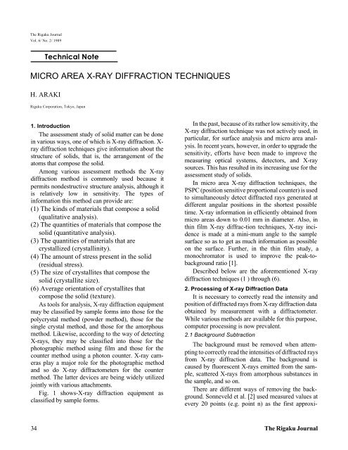
MICRO AREA X-RAY DIFFRACTION TECHNIQUES - Rigaku

The Rigaku Journal 

Vol. 6/ No. 2/ 1989 

Technical Note 

MICRO AREA X-RAY DIFFRACTION TECHNIQUES 

H. ARAKI 

Rigaku Corporation, Tokyo, Japan 

1. Introduction 

The assessment study of solid matter can be done 

in various ways, one of which is X-ray diffraction. X- 

ray diffraction techniques give information about the 

structure of solids, that is, the arrangement of the 

atoms that compose the solid. 

Among various assessment methods the X-ray 

diffraction method is commonly used because it 

permits nondestructive structure analysis, although it 

is relatively low in sensitivity. The types of 

information this method can provide are: 

(1) The kinds of materials that compose a solid 

(qualitative analysis). 

(2) The quantities of materials that compose the 

solid (quantitative analysis). 

(3) The quantities of materials that are 

crystallized (crystallinity). 

(4) The amount of stress present in the solid 

(residual stress). 

(5) The size of crystallites that compose the 

solid (crystallite size). 

(6) Average orientation of crystallites that 

compose the solid (texture). 

As tools for analysis, X-ray diffraction equipment 

may be classified by sample forms into those for the 

polycrystal method (powder method), those for the 

single crystal method, and those for the amorphous 

method. Likewise, according to the way of detecting 

X-rays, they may be classified into those for the 

photographic method using film and those for the 

counter method using a photon counter. X-ray cameras 

play a major role for the photographic method 

and so do X-ray diffractometers for the counter 

method. The latter devices are being widely utilized 

jointly with various attachments. 

Fig. 1 shows-X-ray diffraction equipment as 

classified by sample forms. 

In the past, because of its rather low sensitivity, the 

X-ray diffraction technique was not actively used, in 

particular, for surface analysis and micro area analysis. 

In recent years, however, in order to upgrade the 

sensitivity, efforts have been made to improve the 

measuring optical systems, detectors, and X-ray 

sources. This has resulted in its increasing use for the 

assessment study of solids. 

In micro area X-ray diffraction techniques, the 

PSPC (position sensitive proportional counter) is used 

to simultaneously detect diffracted rays generated at 

different angular positions in the shortest possible 

time. X-ray information in efficiently obtained from 

micro areas down to 0.01 mm in diameter. Also, in 

thin film X-ray diffraction techniques, X-ray incidence 

is made at a minimum angle to the sample 

surface so as to get as much information as possible 

on the surface. Further, in the thin film study, a 

monochromator is used to improve the peak-tobackground 

ratio [1]. 

Described below are the aforementioned X-ray 

diffraction techniques (1 ) through (6). 

2. Processing of X-ray Diffraction Data 

It is necessary to correctly read the intensity and 

position of diffracted rays from X-ray diffraction data 

obtained by measurement with a diffractometer. 

While various methods are available for this purpose, 

computer processing is now prevalent. 

2.1 Background Subtraction 

The background must be removed when attempting 

to correctly read the intensities of diffracted rays 

from X-ray diffraction data. The background is 

caused by fluorescent X-rays emitted from the sample, 

scattered X-rays from amorphous substances in 

the sample, and so on. 

There are different ways of removing the background. 

Sonneveld et al. [2] used measured values at 

every 20 points (e.g. point n) as the first approxi- 

34 The Rigaku Journal

Vol. 6 No. 2 1989 35

mation of the background. But in view of a likelihood 

that some of the selected points fall on diffraction 

lines, they conceived sample P i (i= 2, 3, . . ., n - 1 ) at 

point n - 2 by removing both ends in order to achieve a 

better approximation. In this case, calculation of (m i-1 

+P i+1 )/2 is to be made, and if Pi > m i , then P i should be 

replaced with m i . 

A smooth curve can be obtained by repeating the 

above procedure several times and sequentially 

connecting each point. This curve is regarded as the 

background and is to be subtracted from the 

measurement data. If the background changes 

forming a curve as shown in Fig. 2(b) instead of 

changing almost linearly in terms of 2θ, then P i >m i +C 

may be used to replace the formula P i > m i . 

There is R. P. Goehner's [3] method as another 

method along with other pertinent ones which have 

been devised according to the memory size and speed 

of computers to be used. 

2.2 Detection of Peak Position and Its Measurement 

Various methods are available for peak position 

determination as well. What is frequently used is one 

by means of a quadratic differential curve of the 

measurement data [4], [5], [6]. (See Fig. 3.) The 

quadratic differential method is advantageous in that 

it allows peak detection even in the case of raw data as 

well as in the case of a peak overlapped with another 

peak at its shoulder, thus making its detection difficult 

by the linear differential method. 

Fig. 2 Background determination. (a) When background 

is roughly a straight line. (b) When background has some 

curvature. 

Fig. 3 Peak detection and positional determination with 

linear and quadratic curves. 

Fig. 4 Example of qualitative analysis result. 


3. General X-ray Diffraction Techniques 

Fig. 5 Difference in calibration curve due to absorption 

coefficient. 

3.1 Qualitative Analysis 

This analytical procedure is the so-called searchmatch 

of X-ray diffraction data, such that the diffraction 

pattern of an unknown sample is measured and is 

compared with already known standard patterns 

(JCPDS cards) to obtain an identification. 

When the unknown sample consists of a single 

material, its qualitative analysis is rather simple. 

When it is a mixture, on the other hand, the analysis 

requires high-level skills because of the many diffraction 

present. A variety of combinations of standard 

patterns should be taken into account. To cope with 

the situation, an attempt to carry out search-match 

with a computer was initiated in the 1960s, and improvements 

have been made year after year. The presentday 

search-match has gone so far as to include a 

search of the complete JCPDS files, comprising over 

48,000 patterns. 

3.2 Quantitative Analysis 

This procedure estimates the quantity of the 

analyte material by taking advantage of the fact that 

the peak heights in an X-ray diffraction pattern are 

proportional to the quantities of materials that compose 

a solid. 

In quantitative analysis by X-ray diffraction, the 

mean mass absorption coefficient depends on the difference 

in the quantity ratio of material, resulting in a 

difference in the diffracted ray intensity. It is important, 

therefore, to correct for absorption due to the 

material. Quantitative analysis techniques are classified 

according to differences in the absorption correction. 

Quantitative analysis may be made in two ways; 

one is the internal standard method designed to mix a 

known quantity of material into an unknown sample, 

and the other is the external standard method designed 

for separate measurement without mixing. Although 

the external standard method is preferable for 

quantitative analysis, errors are liable to occur in this 

method. For this reason, the internal standard method 

is more often used. 

3.3 Crystallinity 

In X-ray diffraction data a pattern due to a crystalline 

material and a pattern due to an amorphous 

material may overlap with each other. They differ as 

shown in Fig. 6. 

While various methods are available for the 

determination of crystallinity, they are basically the 

same. That is, they employ a way of examining the 

degree of crystallinity from a ratio between the 

Fig. 6 When crystalline material and amorphous material area mixed together. 

Vol. 6 No. 2 1989 37

Fig. 7 Uniform distortion and nonuniform distortion. 

Fig. 8 Stress and lattice interplanar spacing. 

pattern area of the crystalline material and that of the 

amorphous material. There is such a case, however, as 

with graphite, for instance, where the position of its 

diffraction line will vary depending on the degree of 

crystalline properties. This is also referred to as 

crystallinity. 

3.4 Residual Stress 

When force is applied solid matter within its 

elastic limit, it will be deformed in proportion to the 

magnitude of the force. In other words, the crystal 

lattice interplanar spacing (d-value) of the material 

will change. This distortion is uniform and it should 

be distinguished from nonuniform distortion referred 

to in Fig. 7. 

When changes in the diffraction angle (2θ) are 

examined by varying the angle ψ formed by the 

normal to the sample plane and that to the lattice 

plane, the stress value can be obtained by using the 

following equation. 

E 

π ∂( 2θ) 

σ = − ⋅cot 

θ 

0 

⋅ ⋅ 

2 

2 1+ 

ν 180 ∂ sin φ 

( ) 

( ) 

= K ⋅ 

∂ 

∂ 

( 2θ) 

( sin 2 φ) 

where 

σ: Stress (kg/mm 2 ) 

E: Young's module (kg/mm 2 ) 

ν: Poisson's ratio 

θ 0 : Standard Bragg angle 

K: Constant determined by material and measurement 

wavelength (called a stress constant) 

The optical system of the stress measuring system 

should be selected according to the shape of the object 

for measurement and the stress measuring direction. 

3.5 Crystallite Size 

The peak width in an X-ray diffraction pattern is 

related to the size of crystallites that compose the 

material. 

Besides minuteness of the crystallite, nonuniform 

distortion of the crystallite (Fig. 7) is another factor 

that causes broadening of the peak width. Accordingly 

the size of the average crystallite can be determined 

by measuring the peak width. Scherrer's equation and 

Hall's equation are often used for calculations of the 

crystallite size. 

(Method by Scherrer) 

K ⋅λ 

Dhkl = 

βcosθ 

where 

λ: X-ray wavelength for measurement (Å) 

β: Breadth of diffracted rays due to the crystallite 

size (rad) 

θ: Bragg angle of diffracted rays 

K: Constant (which differs depending on β and 

D constants) 

(Method by Hall) 

λ 

β = β1 + β2 = + 2ηtanθ 

ε cosθ 

βcosθ 

sinθ 

1 

∴ = 2η 

+ 

λ λ ε 

where 

β 1 : Integral width of the breadth of diffracted rays 

due to the crystallite size (rad) 

β 2 : Integral width of nonuniform distortion η, the 

relation with the nonuniform distortion is: β 1 = 2 

tan θ 

ε: Crystallite size (rad) 


The gradient of a straight line obtained by plotting 

βcosθ/λ and sinθ/λ on the Y-axis and X-axis 

respectively, is 2η. The point of intersection with the 

Y-axis is 1/ε. From this, calculation can be made by 

separating the ununiform distortion η and the crystallite 

size from each other. 

3.6 Texture 

When the crystal orientation of matter that 

composes a solid is random, the resultant Debye rings 

will be uniform, as shown in Fig. 11 (a), (b), (c). If, on 

the other hand, the crystal orientation is in a particular 

direction, an arc shape will result instead of a ring, as 

shown in Fig. 11 (d). Such a state is referred to as 

preferred orientation. 

Sometimes there are cases in which preferred 

orientation is specifically given to utilize texture in 

order to improve the characteristics of solid materials. 

The device to measure the state of this texture is a pole 

figure diffractometer attachment. 

Fig. 9 Example of residual stress calculation result. 

RESULTS OF STRESS ANALYSIS 

PEAK POSITION : CENTER OF FWHM 

STRESS = -0.36 kg/mm/mm 

SIGMA RELIABILITY = +-0.04 kg/mm/mm 

4. Assessment of Materials by X-Ray Diffraction 

Techniques 

The aforementioned items 3.1 through 3.6 serve as 

basic assessment methods to examine the state and 

quality of solid matter. By way of example, one of the 

methods used for analysis of the mechanical behaviors 

of materials is shown in Fig. 13. 

5. Other X-ray Diffraction Techniques for Material 

Assessment 

The above descriptions have been made centered 

on bulk analysis. In general X-ray diffraction 

techniques there are certain systems in which the X- 

Fig. 10 Particle size and crystallite size. 

Fig. 11 Observation of Debye rings in polycrystals: α-Fe (211). 

Vol. 6 No. 2 1989 39

Fig. 12 Measurement example with a pole figure attachment. 

Fig. 13 Relations of material information and X-ray diffraction techniques. 

ray optics, detector and X-ray source are specifically 

deisgned for particular applications, such as: 

• Thin film X-ray diffraction method [1] 

• X-ray surface diffraction method [7] 

• Cone scanning type microdiffractometer 

• Curved PSPC type microdiffractometer (PSPC/ 

MDG) 

• Small angle scattering measurement method 

etc. 

These methods are aimed at surface analysis, 

micro area analysis and the like. In any case the 

existence of preferred orientation must be taken into 

account. 

Because the number of crystallites that contribute 

to diffraction in lessened in the case of micro area X- 

ray diffraction techniques, this may cause discontinuous 

Debye rings. For the purpose of getting a 

measurement result with high reproducibility by 

eliminating this drawback, rotation or oscillation is 

applied to the sample during measurement. Three 

axes ω, χ and θ are available as the axis of these 

movements, and they can be run independently or 

simultaneously to perform the desired rotation or 

oscillation. 

The small angle scattering measurement method 

deals with diffuse scattering caused in the vicinity of 


the incident X-ray direction as well as Bragg 

reflections in case of exceedingly large lattice 

interplanar spacing. It deals also with a phenomenon 

that diffraction due to long periodicity is observed 

when the crystalline properties and the amorphous 

properties are arranged periodically in fiber samples. 

These are utilized for particle size measurement, longperiodicity 

measurement, and so on. 

6. Conclusion 

In recent years, higher-intensity X-ray sources 

have become available, such as synchrotron radiation 

X-rays from an electron storage ring and X-rays from 

a high-power rotating anode X-ray generator. 

Moreover, the improvement and progress in 

measurement methods now make it possible to 

conduct structure analysis of micro area objects for 

measurement under various conditions by X-ray 

diffraction techniques. 

Fig. 14 Measurement example with a thin film attachment. 

Fig 16. .Measurement example with PSPC/MDG. 

Fig. 15 Measurement example of a rock flake. 

Fig 17. Sample moving axes in curved PSPC/MDG. 

Vol. 6 No. 2 1989 41

Fig. 18 Effect of 3-axis oscillation 

References 

[ 1 ] Kobayashi and Yoshimatsu: Progress of X-Ray Analysis 

VII, Kagaku Gijutsu-sha (1975), 49. 

[ 2 ] E. J. Sonnevied and J. W. Vieser: L. Appl. Cryst., 8 

(1975), 1 . 

[ 3 ] R. P. Goehner: Anal. Chem., 50 (1978), 1223. 

[ 4 ] A. Savitzky and M. J. E. Goley: Anal. Chem., 36 (1964), 

1927. 

[ 5 ] M. A. Mariscotti: Nuclear Instruments and Methods, 50 

(1967), 309. 

[ 6 ] W. N. Schreiner and R. Jenkins: Adv. X-ray Analysis, 23 

(1980), 287, 

[ 7 ] Kikuta: J. of The Crystallographic Society of Japan, 29 

(1987), 44.

MICRO AREA X-RAY DIFFRACTION TECHNIQUES - Rigaku

You also want an ePaper? Increase the reach of your titles

Delete template?

Save as template?