Sonar Acoustics Handbook

1959 - 2009
Celebrating fifty years ofNURC
accomplishments in the application of
science to NATO operational requirements
© NURC, 2008

Sonar Acoustics
Handbook
NURC. La Spezia,Italy. 2008

Preface
PREFACE
This handbook is a quick guide to the use of sonars for both
mi litary and civi lian purposes. The effect of the ocean environment
on acoustic propagation is illustrated, and practical
results for each term in the sonar equation related to
the environment (propagation, noise, reverberation), to the
acoustic source and the target, and to array and signal processing,
are provided in graph ical or tabu lar fann. Thi s
han dbook should be of interest to both scientists and engineers
worki ng with sound in the ocean.
Finn B. Jensen
March 2008

Contents
TABLE OF CONTENTS
FU;\DA~IE:"TALU:"ITS
International System of Units
SI Base Units ..
SI Derived Units .
Prefixes for SI Units.
Conversion into SI Units
Intensity and Decibels .
Spectrum Level .. .
SONAR EQUATIONS
Definition of Sonar Equat ions .
Definition of Parameters . ..
Combin ations of Sonar Parameters
Passive Sonar Equation . . . . . .
Ac tive Sonar Equati on .
Frequency Ranges of Sonar Applications .
GE:"ERATIO:" OF SOU:"D
Source Level . . . . . . . .
Transm itter Directivity Index . . . . . .
Source Level and Radiated Acoustic Power
I
I
I
I
2
2
4
4
6
6
6
8
8
8
8
9
9
9
9
PROPAGATIO~
Acoustic and Wave Propagation Tenns
Sound Speed in Seawater .
Sound Speed in Bubbly Water
Sound Speed Profiles
Propagation Examples ... . .
Sound Attenuation in Seawater
Bottom Loss . . . .
Transm ission Loss .
II
II
14
14
16
18
24
25
30

Contents
AMBIENT NOISE
Noise Tenns . . . . . . . .
General Overview. . . . .
Wind and Shipping Noise
REVERBERATION
Rayleigh Scattering . . . . . .
Scattering Strength Parameter
Sea Surface Reverberation
Bottom Reverberation .
Volume Reverberation.
TARGET STRENGTH
Scattering Cross Section
Scattering by Rigid Sphere
Scattering by Air Bubble .
Target Strength of Simple Bodies
Target Strength of Complex Objects
ARRAY RESPONSE
Directivity Index and Directivity Factor
Unifonn Line Array. . . . . . . . . . .
Unifonn Line Array with Shading . . .
Linear Array of Equispaced Transducers.
Synthetic Aperture Sonar . . . . . . . . .
32
32
32
33
36
36
36
31'
38
40
43
43
43
46
48,
49
50
50
51
52
54
55
I
DETECTION THRESHOLD 60
Sonar Receiver Signal Processing 60
Definitions. . . . . . . . . . . . . 60
Detection Thresholds for Standard Sonar
Signals. . . . . . . . . . . . . . . .. 61
Detection Thresholds for Optimum Processor 65

Contents
SIGNAL ANALYSIS 66
Frequency Analysis Terms 66
Harmonic Analysis . . . . 71
Octave and Third-Octave Filters 71
Logarithmic vs Linear Amplitude Scale 73
Time-Bandwidth Product 73
Confidence Limits . 74
Doppler Shift . . . . 74
Ambiguity Function . 75
DIVERS AND MARINE MAMMALS:
SAFETY LEVELS 77
Military Divers . . 77
Recreational Divers 78
Marine Mammals 78
REFERENCES 80
SUBJECT INDEX 81
ACKNOWLEDGMENTS 84

Fundamental Units
FUNIIAMEi\TAL UNITS
lnrcrnutioual System of Units
The International System of Units (SI) established in 1960
is based upon: The meter (m) for length; the kilogram
(kg) for mass; the second (s) for time; the Kelvin (K) for
temperature; the ampere (A) for electric current; and the
cande la (cd) for luminous intensity. All other units of the
51 system are derived from these base units.
SI Base Units
Quant ity Unit Symbol
Length meter m
Mass kilogram kg
Time second s
Temperature kelvin K
Electric current ampere A
Luminous intensity candela cd
51 Dertved Units
Quantity Unit Symbol Formula
Acceleration
m/s:!
,
Area
m-
Density
kg/m'
Energy joul e J N-m
Force newton N kg-m/s"
Frequency hertz Hz lis
Power watt W J/s
Pressure pascal Pa N/m:!
Velocity
mls
Volume
m'

2
Fundamental Units
Prefixes for 51 Units
Prefix Sym bol Factor Prefix Symb ol Factor
deci d 10 ' dek. d. 10 '
centi c 10- 2 hccro h 10 2
milli m 10- 3
kilo k 10 3
micro p 10- 6 mega M 10 6
nana n 10- ' giga G 10'
pico P
10- 12
tera T 10 12
femto f 10- 15
peta P 10 15
ano a 10- 18
exa E
lOIS
Conversion into SI Uni ts
Quantity Unit Formula
Length inch 1 in - 0.0254 m
foot
1 ft = 12 in = OJ 048 m
yard
I yd = 3 ft = 0.9 144m
fathom 1 fm = 6 ft = 1.8288m
mile (statute) 1mi = 1.609 km
mile (nautical) 1nm = 1.852 km
Area square inch I in l ~ 6.45 16 ·IO~4 m 2
square foot 1ft' = 0.0929m'
square yard I yd' = 0.836 1m'
square mile 1mil = 2.5900 km'
square mile I nrrr' = 3.4299 km 2
Volume cubic inch 1in) = 1.6387-10 5 m'
cubic foot 1 ft3 = 2.83 17·10-' m'
cubic yard I yd' = 0.7646 m J
liter Ii = 10- 3 m'
quart I qt = 0.9464e
ga llon (US) 1gales = 3.785l
ga llon (UK) I gal es; = 4.546 l

Fundamental Units 3
Quantity Unit Formula
Velocity foot/second 1 fl/sec - 0.3048 mls
knot 1kt ~ 1 nmlh ~ 0.5144 m1s
mile/hour 1 mi/hr = 1.609 kmlh
Mass ounce I oz - 2.835· 10-' kg
pound l ib ~ 160z ~ 0.4536kg
Force pound force I Ibr - 4.44 8 N
Energy calorie 1cal - 4.187J
foot-pound 1 ft-Ibr ~ 1.356 J
Power horse power 1hp - 550 ft-lbr - 745.7 W
Pressure atmosphere I atm - 1.013·10' Pa
bar I bar = lOs Pa
psi Ilbr/in' = 6.895 ·10' Pa
psf I lbrlft' ~ 47.88 Pa
Temp C to K K - C + 273.15
of to °c C = (F - 32)/1.8
Celcius
('C)
Fahrenheit
(OF)
Kelvin
(OK )
Boiling point +100 °c
(water)
+373.15 oK
Body temp. +37 °C +98.6 of +310.15 °K
Freezing DoC +32 of +273.15 °K
point _17.78 °C oof +255.37 oK
, , ,
Absolute __ - 273.15 "c .-459.67 of
zero
'"
OOK
FBJ

4
Fundamental Units
Intensity and Decibels
The decibel (dB) is the dominant unit in sonar acoustics
and denotes a ratio of intensities (not press ures) expressed
in terms of a logarithmic (base 10) scale. Two intensities
I I and / 2 have a ratio h I!:;! in decibels of 10 Jag lo (J II/ 2)
dB. Absolute intensities can therefore be expressed by using
a reference intensity. The presently accepted reference
intensity is that of a plane wave having a root-mean-square
(nn s) pressure equa l to 10- 6 pasca ls or a micropascal
(u Pa). Therefore, taking I,u Pa as the reference sound pressure
level, a sound wave having an intensity of, say, one
million times that of a plane wave of rms pressure l .uPa
has a level of 10 Iog IO ( 10') " 60 dB re 1p Pa.
Pressure (P) ratios are expressed in dB re I p Pa by taking
20 log 10 (PIfp 2 ) where it is understood that the reference
originates from the intensity of a plane wave of pressure
equal to I I-J Pa.
The average intensity I of a plane wave with rms pressure p
in a medium of density p and sound speed c is I = p2fpc.
In seawater, pc is I. 5 x 10 6 kg/(m 2s) so that a plane wave of
nn s pressure I p Pa has an intensity of 0.67 x 10- 18 W/m 2
(i.e., 0 dB re I I' Pal.
The above discussion has direct application to continuous
wave (CW) signals. For broadband signa ls or noise, the
acoustic intensity must be referred to a bandwidth and generally
the reference bandwi dth is I Hz. Hence, the spectrum
level is expressed in units of dec ibels referenced to
a micropascal in a I-Hz band and sometimes written as
dBffp Pa 2 / Hz. A source spectrum level must also have a
reference distance so that an example of the unit of source
spectrum level is dB ffpPa 2 / Hz @ 1 m.
In the above cases, the spectral level is for a squared quan-

Fundamental Units 5
tity such as intensity for which decibels are a natural unit.
In the case of amplitude, we must still refer to a ratio of
intensities so that the units of the corresponding spectral
amp litude level would be dB llpPa / .JHZ.

Ii
Sonar Equations
SONAR EQUATIONS
Definition of Sonar Equations
The sonar equations are a logical basis for the prediction
of performance of sonar equipment and form a framework
for the design of sonar equipment with a specified level of
performance.
Definition of Parameters
SL:
NL:
or:
TL:
AN:
TS:
SL:
AG:
RL:
RD:
Equipment Parameters
Projector Source Level
Self Noise Level
Receiving Directivity Index
Medium Parameters
Transmission Loss
Ambient Noise Level
Target Parameters
Target Strength
Target Source Level
Additional Parameters
Array Gain
Reverberation Level
Recognition Differential
Parameters of the sonar equations are always expressed In"
decibel units.
Ambient Noise Level. That part of the total background
noise level observed with an omnidirectional hydrophone
which is not due to the hydrophone and its mounting; usually
reduced to a I-Hz frequency band and referred to as
an ambient noise spectrum level.
Array Gain. A measure of the change in signal-to-noise
ratio (SNR) which results from the use of an array of hy-

Sonar Equations 7
drophones instead of a single phone. Array gain is defined
by
AG = 10 10glo(SNRA / SNR H),
where SNR A is the signal-to-noise measured at the array
terminals and SNR 1-1 is measured at a single hydrophone.
Projector Source Level. The intensity ofthe radiated sound
in decibels relative to the intensity of a plane wave of rms
pressure I .uPa referenced to a point I ill from the acoustic
center of the projector in its peak response direction.
Receiving Directivity Index. Ratio, in decibel units, of the
power output of the array to the power output ofan omnidirectional
hydrophone, referenced to a unidirectional plane
wave signal in an isotropic noise field and for the array
steered in the direction of the signal.
Recognition Differential. Ratio, in decibel units, ofthe signal
power in the receiver bandwidth to the noise power in
a I-Hz band, measured at the receiver terminals, required
for detection at some pre-assigned level of correctness of
the detection decision.
Reverberation Level. Ratio, in decibel units, of the acoustic
intensity produced by reverberation to the acoustic intensity
produced by a plane wave of rms pressure I pPa.
Self Noise Level. A particular kind of background noise
occurring in sonars installed in a noisy vehicle, usually
reduced to a I-Hz frequency band and referred to as a
spectrum level.
Target Source Level. Similar to projector source level except
that the target causes the disturbance.
Target Strength. Ratio, in decibel units, of the sound returned
by the target at a distance of I m from its acoustic
center, to the incident intensity from a distant source.
Transmission Loss. Ratio, in decibel units, of the acoustic
intensity of the source measured at 1 m distance from
its acoustic center, to the acoustic intensity received at a
distant point.

8
Sonar Equations
Cnmhinatinns (If Sonar Parameters
Name
Echo Level
Figure of Merit
Noise Masking Level
Performance Index
Reverberation Masking Level
Parameters
SL - 2TL + TS
SL - (NL - DI + RD)
NL- DI +RD
TL + AN - AG
RL+RD
Passive Sonar Equation
SE = SL - TL - AN + AG - RO
Active Sonar Equation
SE = SL - 2T L + TS - RL - RD
where SE denotes signal excess, the decibel difference between
signal-to-noise ratio and the recognition differential.
If an active sonar is self noise limited, RL is replaced by
NL- 01. The use of recognition differential in the sonar
equations above implies that the masking term, AN or RL,
needs to be expr essed on a per Hz basis,
Frequency Ranges of Sonar Applications
1 10 100 l k 10k lOOk 1M
'AdjU' lIciil oce··ilcjg"'PJ'y
~llijiViiyTriQ
- Ecl!9-!.'1\Ill _~ G
_
lo1~ ~lOfi
" hfng
l
Mil' Y B..Wr,ll9!' r
:: _.~ ;(J~"rY-paso.vo iilMr
l~ fiai!il utj"~ M itilii-'lDund_ l!1t1~~ n ~
10 100 Ik 10k
Frequency (Hzl
1M

Generation ofSound
')
Source Level
GENERATION OF SOUND
In the sonar equations, source level is a measure of the
sound power radiated by the acoustic transmitter. Source
level is defined as the intensity ofradiated sound in decibels
relative to the intensity of a plane wave of rms pressure
IpPa, referenced to a point 1m from the acoustic center of
the transmitter in the direction of the target.
Transmitter Directivity Index
The directivity index DrT ofa transmitter is the difference
between the level ofsound generated by a directional source
in the direction of the target and the level that would be
produced by an omnidirectional source radiating the same
total amount of acoustic power, i.e.
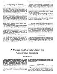
Source Level and Radiated Acoustic Power
The source level SL of a transmitter is related in a simple
way to the acoustic power PT that it radiates and to its
directivity index. The average intensity I of a plane wave
with rms pressure p in a medium of density p and sound
speed c is I = p 2/pc . The total radiated power is obtained
by integrating over the surface of a sphere of radius r ,
2
P T = L 41rr 2
pc

10 Generation ofSound
Converting into decibels with r = 1 m and remembering
that 10 logpt expressed in I'Pa is the source level SL. we
get
10 loglo PT = SL + 10 10gID (~: 10- 12 ) .
Now insert p = 1000 kg/rrr' and c = 1500 mls for seawater
to obtain
SL = 170 .8 + 10 10gi0 PT
[dB re I pPa @ l m],
where the acoustic power is given in watts . If the transmitter
is directional with a directivity index Dl-r, the final
expression for the source level becomes
SL = 170 .8 + 10 log ID PT + Dlj,
which is graphed below for selected values of Dl r .
240
230
1
'&
::l. 220 '
e
m 210 '
~
0;
~
lBO
10 100 1000
Acoustic power output (yVl
10000
The radiated acoustic power ofshipboard sonars range from
a few hundred watts to some tens of kilowatts with directivity
indexes between 10 and 30 dB. It follows that the
source levels of shipboard sonars arc in the range 210 to
240dB.

Propagation
11
I'ROP;\(;:\TIO.'\;
Acoustic and Wave l'ropaguriou Terms
Absorption. The conversion of sound energy into another
form of energy, usually heat, when passing through an
acoustic medium.
Acoustics. The science of the production, control, transmission,
reception and effects of sound.
Adiabatic . Without gain or loss of heat.
Attenuation. Propagation of acoustic waves is always associated
with energy loss due to absorption, i.e, the transfer of
energy into heat. Moreover, sound is scattered by medium
inhomogeneities, also resulting in a decay of sound intensity
with range. Generally, it is not possible to distinguish
between absorption and scattering effects; they both contribute
to sound attenuation in a real medium.
Body waves. Waves that propagate through an unbounded
continuum, as opposed to surface or interface waves, which
propagate along a boundary between two media.
Caustic. The envelope of rays formed after either reflection
or refraction associated with intense focusing of energy. A
convergence zone is a specialized type of caustic occurring
near the sea surface in deep water under favorable propagation
conditions.
Cavitation. Sound-induced cavitation in a liquid is the formation,
growth, and collapse of gaseous and vapor bubbles
due to the action of intense sound waves.
Decibel scale. The decibel (dB) is the dominant unit in
sonar acoustics and denotes a ratio of acoustic intensities
expressed in terms of a logarithmic (base 10) scale.
Diffi"action. Penetration of energy into areas forbidden by
geometric acoustics, e.g. the bending of wave energy around
objects or into shadow zones. Diffraction is strongest when
the acoustic wavelength is comparab le to, or larger, than the
object. Diffraction can be explained by Huygens' principle
and is predictable by a full wave theory solution.

12 Propagation
Dispersion. When the phase speed is dependent on frequency.
Two types of dispersions are important in sonar
acoustics: (i) Geometrical dispersion in a waveguide, which
causes modal phase velocities to become frequency dependent;
(ii) Intrinsic dispersion, which is present in all real
media with attenuatio n. The phase (sound) speed is then
weakly frequency dependent even in homogeneous media
without boun daries .
Dissipation. Loss of acous tic energy into heat. Equivalent
to absorption.
Geop hone. A transducer used in seismic work. When it is
placed in the ground it responds to any displac ements of
the ground caused by the pass age of elastic waves arising
from earthqu akes, seismic shots, explosions, ere.
Group velocity. The velocity of a wave disturbance as a
whole, i.e. of an entire group of component simple harmonic
waves. The group velocity V g is related to the phase
velocity V p of the individual harmonic waves of wavenumber
k = 271:f/Vp , as dt/.
Vg = Vp + k d: '
wheref is the frequency. The group velocity is thus equa l
to the phase velocity only in the case of nondispersive
waves, i.e. when d"''/dk = O. The group velocity is an
important concept for waveguide propagat ion. since it is a
measure of the transfer of energy through the waveguide.
Hydrophone. An electro-acoustic transducer that responds
to waterborne sound waves and delivers essentially equivalent
electric waves. The conversion of sound energy into
electrical energy is usually achieved through the use of either
piezoelectric or magnetostrictive materials.
lnfrasound. Sound at frequencies below the audible range,
i.e. below about 20 Hz.
p-wave. A compressiona l body wave in an elastic medium,
with p denoting "p rimary." The particle displacement is
parallel to the direction of wave propagation. For this reason
p -waves are also called longitudinal waves.

Propagation 13
Phase velocity. The speed of propagation ofa point of constant
phase of a simple harmonic wave component given
by lip = co/k, where w = 2][1 is the angular frequency
and k is the acoustic wavenumber. For unbounded homogeneous
media, the phase velocity is equal to the medium
sound speed.
Rayleigh wave. A surface wave associated with the free
surface of a solid. The wave is of maximum intensity
at the surface and decreases exponentially away from the
surface into the solid.
s -wave. A shear body wave in an elastic medium , with
s denoting "secondary." The particle displacement is perpendicular
to the direction of wave propagation. For this
reason s -waves are also called transverse waves.
Scholte wave. An interface wave of the Stoneley type associated
with the interface between a fluid and a solid
medium. The wave is of maximum intensity at the interface
and decreases exponentially away from the interface
into both the fluid and the solid medium.
Sonar. The method or equipment for determining, by underwater
sound, the presence, location, or nature of objects
in the sea. The word "sonar" is an acronym derived from
the expression "SOund NAvigation and Ranging."
Stoneley wave. An interface wave associated with the interface
between two solid media. The wave is of maximum
intensity at the interface and decreases exponentially away
from the interface into both solids.
Ultrasound. Sound at frequencies above the audible range,
i.e. above about 20 kl-lz.
Wavelength. The distance measured perpendicular to the
wavefront in the direction of propagation between two successive
points in the wave, which are separated by one
period. The wavelength X relates to sound speed e and
frequence 1 as X = elf.
Wavenumber. k = 2n:/X, where 1 is the acoustic wavelength.

14 Propagation
Sound Speed in Seawater
The sound speed in the ocean is an increasing function of
temperature, salinity and pressure, the latter being a linear
function of depth. A simple expression for this dependence
is
where
C = 1449.2 + 4.6 T - 0.055 T 2 + 0.00029 T 3
+(1.34 - 0.010 T)(S - 35) + 0.016Z .
c is the sound speed in mis,
T is the temperature in DC,
S is the salinity is part per thousand (ppt),
Z is the depth in m.
This equation, which is valid for 0 :::: T :::: 35 °C, 0 s S s
40 ppt, and 0 :::: Z :::: 1000 m, has been graphed on p.15
for Z = 0 and with the salinity S as a parameter. Note
that the sound speed increases by 1.6 mls per 100 m depth
increase.
In shallow water, where the depth effect on sound speed
is small, the primary contributor to sound speed variations
is the temperature. Thus, for a salinity of 35 ppt,
the sound speed in seawater varies between 1450 mls at
o°c to 1545m1s at 30°C.
Sound Speed in Bubbly \Vatel'
In high sea states the upper ocean may have a significant
infusion of air bubbles down to a depth of 10-20m. Although
the volume fraction of air is relatively small, usually
a small fraction of one percent, the effect of small air concentrations
on the speed of sound is profound. When all
bubbles are small compared to the resonant size (low frequencies),
the sound speed in bubbly water is given by the
simple mixture theory as
_ (pw

Propagation 15
1540 ,-- - - - - - - - - ----,.....----:;--=-..:7 1
1520
~ 1500
1
-g 1460

16 Propagation
15001'"=:::.::--:- - -..-;:= = = = = :.:.:;"]
-- Bubbly rnixiure
_ .- Ail
o"I __~-_-'-;-_
10 5 __':;;-_--'
10
I~' 10
Volume fraction (II
pointed out that gas bubbles may also play an effect in the
seabed, where gas can be generated by biological decay
processes.
Sound Speed Profiles
Seasonal and diurnal changes affect the oceanographic parameters
in the upper ocean. In addition, all of these parameters
are a function of geography. The figure on p. 17
shows a typical set of sound-speed profiles indicating greatest
variability near the surface as function of season and
time of day. In a warmer season (or warmer part of the
day), the temperature increases near the surface and hence
the sound speed increases toward the sea surface. This
near-surface heating (and subsequent cooling) has a profound
effect on surface-ship sonars. Thus the diurnal heating
causes poorer sonar performance in the afternoon-a
phenomenon known as the afternoon effect. The seasonal
variability, however, is much greater and therefore more
important acoustically.
In non-polar regions, the oceanographic properties of the
water near the surface result from mixing due to wind and
wave activity at the air-sea interface. This near-surface
mixed layer has a constant temperature (except in calm,

Propagation 17
o
100 0
I
R 2000
a>
o
Sound speed (mls)
1460 1500 1540 1560
·~-.....L---"r------''--~-----'
\ , \
Surface / '"
duct
pl Onte
\
\
",
\
/ ,
Palm"
region ,
profile ' ,
, ,,
, ,,,,,
Mixed layer
Main thermoc line
warm surface conditions as described above). Hence, in
this isothermal mixed layer we have a sound -speed profile
which increases with depth because of the pressure gradient
effect, the last term in sound speed formula. This is the
surface duct region, and its existence depends on the nearsurface
oceanograph ic conditions. Note that the more agitated
the upper layer is, the deeper the mixed layer and the
less likely will there be any departure from the mixed-layer
part of the profile depicted in the figure. Hence, an atmospheric
storm passing over a region mixes the near-surface
waters so that a surface duct is created or an existing one
deepened or enhanced.
Below the mixed layer is the thermocline where the temperature
decreases with depth and therefore the sound speed
also decreases with depth. Below the thermocline, the temperature
is constant (about 2°C-a thermodynam ic property
of salt water at high pressure) and the sound speed
increases because of increasing pressure. Therefore, be-

18 Propagation
tween the deep isothermal region and the mixed layer, we
must have a minimum sound speed which is often referred
to as the axis of the deep sound channel. However, in polar
regions, the water is coldest near the surface and hence
the minimum sound speed is at the ocean-air (or ice) interface
as indicated in the figure on p. 17. ~n continental
shelfregions (shallow water) with water depth of the order
of a few hundred meters, only the upper part of the soundspeed
profile in the figure is relevant. This upper region
is dependent on season and time of day, which, in tum,
affects sound propagation in the water column.
Propagation Examples
The principal characteristic of deep-water propagation is
the existence of an upward-refracting sound-speed profile
which permits long-range propagation without significant
bottom interaction. Hence, the important ray paths are either
refracted refracted or refractedsurface-reflected. Typical
deep-water environments are found in all oceans at
depths exceeding 2000 m. Illustrative ray diagrams of characteristic
deep-water propagation scenarios as well as a
shallow-water summer scenario are shown on pp. 19-23 .

CONVERGEI\CE ZONE PROPAGATION
~
.g
~ :?.
o·
::
'0
0
SD = 20m
100 0
~
~ 2000
.c
-+-'
0.. 3000
Q)
0
4000
~OOO
1490
SV

20 Propagation
o ọ
...
Cl>
Q1
C
o 0
S'O::
. 0
'"

Propagation 21
rrv."'""lrr----------, ~
z
"""
::::
~
-<
c
;::
""" '-'
::::::
'"
~
v
~
:=
"'" ~ E
-< 0
:...
::::::
....J
.r:
'

22 Propagation
Q)
CJ'
C
o 0
... 0::
E
o
o
N
D
Cl) 1":""=-- -,-- _ -.- _ - -.--__--+ g
~ : ~
o 0 0 0 o ~
o 0 0 a
...... N n
(w ) 4td&O

SHALLOW WATER PROPAGATIO"," (summer)
100 1500 1550 5 10 15 20
SV (m/s) Range (km)
'"tl
C5
~ ....
c'
::l
tv Vol
0
.......... 20
E
40
.c
Q. 60
ill
0 80

24
Propagation
Sound Attenuation in Seawater
When sound propagates in the ocean, part of the acoustic
energy is continuous ly absorbed, i.e., the energy is transformed
into heal. Moreover, sound is sca ttered by different
kinds of inhomogeneities, also resulting in a decay ofsoun d
intensity with range. As a nile, it is not possible in real
ocean experiments to distinguish between absorption and
scatteri ng effects; they both contribute to sound attenua­
(ion in seawater.
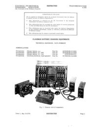
The frequency dependence of attenuation can be roughly
divided into four regimes of different physical origin as displayed
in the figure below. The lowest frequency regime,
region I, is still not completely understood but it is conjectured
that it is related to low-frequency propagation-duct
cutoff, or in other words, leakage out of the deep sound
channel. The main mechanisms associated with regions II
and III are chemical relaxations of boric acid B(OH») and
magnesium sulphate MgS0 4, respectively. Region IV is
dominated by the shear and bulk viscosity associated with
salt wa ter (curve AA'). For reference, also the viscous loss
associated with fresh water is shown as curve BB ' in the
figure.
A simplified expression for the frequency dependence (f
in kHz) of the attenuatio n in dBlkm is,
with the four terms sequentially associated with regions I
to IV in the figure. The above expression applies for a
tempe rature of 4 °e, a salinity of 35 ppt, a pH of 8.0, and
a depth of about 1000 m, where most of the measurement s
on which it is based were made.
In summary, the attenuation of low-frequency sound in
seawater is very sma ll. For instance, at 100 Hz a tenfold
reduction in sound intensity (- 10 dB) occurs over a
distan ce of around 2200 km. Even though attenuation in-

Propagation 25
Region
Leakage
Region
II
Chemical
relaxation
B (01-1) 3
R I Shear & Volume
e9 on viscosity
III
IV
Mg S0 relaxation 4 I .,//
oB'
............/-
1
10
}1
/ /
/ I
/ I
-:.J _ L /
/ /
/
/
/
/
/
/
10- 1 100 10 1 10 2
Frequency (kHz)
creases with frequenc y ( r - I OdB ~ 145 Ian at 1 kHz and
~ 9 km at 10 kHz) , no other kind of radiation can compete
with sound waves for long-range propagation in the
ocean . Electromagnetic waves, including those radiated
by powerful lasers, are absorbed almost completely within
distances of a few hundred meters.
F ())
Reflectivity, the ratio of the amplitudes ofa reflected plane
wave to a plane wave incident on an interface separating
two media, is an important measure of the effect of the
bottom on sound propagation. Ocean bottom sediments
are often modeled as fluids which means that they support

26
Propagation
,
z
IRI
loss le..
l~
o,
00 30 60 9Q • 01
only one type of sound wave-a compressional wave.
The expression for reflectivity at an interface separating
two homogeneous fluid media with density Pi and sound
speed c., i == 1. 2, was first worked out by Rayleigh as
R = Z2 - Z.
Z 2 + Z l '
where Z i '" Pic, I sin 8 i is the effective impedance. Introducing
Snell's law of refraction
k l cos 8 1 = k 2 cos 82.
where k, '" os/c], the reflection coefficient as a function
of the incident grazing angle OJ takes the foml
R (0i ) =
(P2 Ipl) sin 01 - V (CI 1CZ )2 - cos? 0 1
(P 2Ipt) sin Ol + V (Ct Ic2)2 - COS 2 0 1
The reflection coefficient has unit magnitude, meaningperf
ect reflection. when the numerator and denominator in
this expression are complex conjugates. This can only
occur when the square root is purely imaginary, i.e., for
cos B t > C . / C2 (total internal reflection). The associated
critical grazing angle below which there is perfect reflection
is found to be
Be = arccos ( ~~ ) .
Note that a critical angle only exists when the sound speed
of the second medium is higher than that of the first.

Propagation 27
A closer look at the expression for R (Eli) shows that the
reflection coefficient for lossless medi a is real for 9 1 > 9 c ,
which mean s that there is loss ( IRI < 1) but no phase shift
associated with the reflection process. On the other hand,
for 9 1 < g e we have perfect reflection (IR I = 1) but with
an angle-dependent phase shift. In the general case of lossy
media (c. complex), the reflection coefficient is complex,
and, consequently, there is both a loss and a phas e shift
associated with each reflection . The figure on p.26 shows
canonical shapes of the reflection curves both for lossless
and lossy media .
Real ocean bottoms are compl ex layered structures of spatially
varying material compos ition. A geo-acoustic model
is defined as a model of the real seafloor with emphasis
on measured, extrapolated, and predicted values of those
material properties important for the modeling of sound
transmission . In general, a geo-acoustic model details the
true thicknesses and properties of sediment and rock layers
within the seabed to a depth termed the effe ctive acoustic
penetration depth. Thus, at high frequencies ( > I kHz),
details of the bottom composition are required only in the
upper few meters of sediment, whereas at low frequencies
« I00 Hz) information must be provided on the whole
sediment column and on propertie s of the underlying rocks.
The information required for a complete geo-acoustic model
should include the following depth-dependent materi al properties
: The compressional wave speed C p , the shear wave
speed c s , the compressional wave attenuation a p , the shear
wave attenuation a ." and the density p. Moreover, information
on the variation of all of these parameters with
geographical position is required.
The amount of literature dealing with acoustic properties
of seafloor materials is vast. As an indication of the many
different types of materi als encountered just in continental
shelf and slope environments, we list in the table on
p.28 indicative geo-acou stic properties of typical seafloor

Lv
00
::p
..2
~
0'
::s
Bottom type p PI/P tv cpk " cp ".) u. p 0: .,
(%) - - (rn/s) (01/s) (dB IJ.I' ) (dB I!..,)
Clay 70 \.5 1.00 1500 < 100 0.2 \.0
Silt 55 1.7 1.05 1575
Sand 45 1.9 1.1 1650
Gravel 35 2.0 1.2 1800
c.,
c.,
c;
( I )
(2)
(3)
1.0 1.5
(U3 2.5
0.6 1.5
Moraine 25 2.1 1.3 1950 600 0.4 1.0
Chalk - 2.2 1.6 2400 1000 0.2 0.5
Limestone - 2.4 2.0 1000 1500 0.1 0.2
Basalt - 2.7 3.5 5250 2500 0.1 0.2
c;1) -= 80 2 0 3
C", =1500 m/s, f! 1V = I000kg/rrr'
e(2) = 1l Oi ll J
c:(3 ) = 180 i o. J

Propagation
29
20 ,-------~--~-----
co
~ 5
til
til
.Q
" 0
tl 10

30 Propagation
Trnnsmlsvinu , 11\\
An acoustic signal trave ling through the ocean becomes
distorted due to muItipath effects and weak ened due to
various loss mechanisms. The standard measure in underwater
acoustics of the change in signal strength with
range is transmission loss defined as the ratio in decibels
between the acous tic intensity I (r, z) at a field point and
the intensity 10 at l- rn distance from the source, i.e.,
TL
-101 l(r,z)
og 10 10
_ 201 Ip (r, z )1
ogl o Ipol
[dB re 1m] .
We have here made use of the fact that the intensity in a
plane wave is proportional to the square of the pressure
amplitude.
Transmission loss may be considered to be the sum of a
loss due to geometrical spreading and a loss due to attenuation.
Th e spreading loss is simply a measure of the signal
weakening as it propagates outward from the source.
The next figure shows the two geometries of importance
in underwater acoust ics. First cons ider a point source in
an unbounded homogeneous medium (left figure). For this
simple case the power radiated by the source is equally distributed
over the surface area of a sphere surro unding the
source. If we assume the medium to be lossless, the intensity
is inverse ly proportional to the surface of the sphere,
i.e., 1

Propagation
31
(a) Spherical spreading (b) Cylindrical spreading
-Gt
°3
tI' "
!
10:_1_ 10:_1_
41tR 2
21lRD
D, i.e., 10: 11(27rRD ). The cylindrical spreading loss is
therefore given by
TL= 1010giO r [dBre 1m] .
Note that for a point source in a waveguide, we have spherical
spreading in the nearfield (r ~ D) followed by a transition
region toward cylindrical spreading which applies
only at longer ranges (r » D).
As an example consider propagation in a waveguide to a
range of 100 km with spherical spreading applying on the
first kilometer. The total propagation loss (neglecting attenuation)
then becomes: 60 dB + 20 dB = 80 dB. This figure
represents the minimum loss to be expected at 100km. In
practice, the total loss will be higher due both to the attenuation
of sound in seawater, and to various reflection and
scattering losses.

32 Ambient Noise
uisc Term,
\ IBll· \ I ,01 r-
Ambient noise. The composite noise from all sources in a
given environment excluding noise inherent in the measuring
equipment and platform.
Cavitation noise. The noise produced in a liquid by the
collapse of bubbles that have been created by cavitation.
Pink noise. Broadband noise where the power spectral density
is inversely proportional to frequency (-3 dB per octave
or -10 dB per decade).
Self noise. The limiting noise registered by a sonar receiver
that is cau sed by the vessel itself or as a result of its motion.
Spectrum level. Ambient noise intensity in dB re I,uPa 2
averaged over a frequency band of width I Hz. In terms of
amplitude, the spectral level is in units of dB re I,uPa /..JHi..
Therm al noise. Minute movements of the water molecules
that are due to thermal agitation accompanied by the release
of acoustic energy. The thermal noise is proportional to the
absolute temperature of the water.
Traffic noise. The ambient noise component which is caused
by shipping.
White noise. Broadband noise where the power spectral
density is constant with frequency.
Wind noise. The noise generated near the sea surface due
to hydrostatic effects of wind-generated waves, whitecaps,
bubble plumes, and direct sound radiation from the rough
sea surface.
Ambient noise results from a number ofnatural phenomena
as well as from man-made activities. Referring to the figure
on top of p. 34, five frequency regions corresponding to
different sources of noise can be distinguished [2]:

Ambient Noise 33
1. Very low frequency (VLF) region from 0.1 to 5 Hz:
Seismic events and non-linear interaction of surface
waves.
2. Low frequen cy (LF) region from 5 to 20 Hz: Wave
turbulence.
3. Shipping from 20 to 200Hz: Distant shipping.
4. Atmospheric influences from 200 Hz to 100kHz:
Wind and wave motion, and precipitation.
5. Thermal noise above 100kHz: Molecular motion.
Note that there is a variation in spectral levels of 2D-30dB
between low-noise and high-noise situations throughout the
entire frequency band of interest. This is due both to variation
in the noise generation mechanisms and due to local
propagation conditions. The peak: intensity occurs around
0.3 Hz (non-linear wave interaction) but there is a spectral
slope of - 5 to - 10 dB/octave the whole way up 100kHz.
Then noise increases again at a rate of +6 dB/octave due
to thermal noise [1].
I
As shown in the lower figure on p. 34, shipping and wind
are the .important sources of noise for sonar applications
in the frequency range 10 Hz to 10kHz. Distant shipping
accounts for ambient noise between 20 and 200 Hz in most
deep water, open ocean areas and in highly traveled seas
such as the Mediterranean. Wind noise dominates above
200Hz and is usually parameterized according to sea state
(also Beaufort number) or wind force. The relationship
between sea state, wind speed, and wave height is summarized
in the table on p.35.

34 Ambient Noise
IF
region
AlmCjsp!leric inlluences
~ 80
~ VLF mgicn
E ~
60
2
tl ;\0
a>
Q.
o»
20 _.. ... .........--- I
Theimal noise>/
. , ,," ,
0 0 1 10 100 lk 10k lOOk
Frequency (Hz)
e - N
J:
.,
100 1 SHIPPING
90
BO
~
70
l!?
LD
~ 60
OJ >
~ 50
E2
40
tl
a> c-
rt> 30
20
10 100 1000 101(
Frequency (Hz)

SEA STATE DESCRIPTION
Beaufort Sea Wind speed Wind speed Wave height Sea description
scale state (kn) (km/h) (m)
0 0 < 1 < 2 0 Like a mirror
1 Ih 1-3 2-6 < 0.1 Ripples are formed
2 1 4-6 7-11 0.1-D.3 Small wavelets
3 2 7-10 12-19 0.3-0.6 Waves begin to break
4 3 11-16 20-29 0.6-1.2 Numerous whitecaps
5 4 17-21 30'-39 1.2-2.4 Moderate waves. some spray
6 5 22-27 40-50 2.4-4.0 Large waves, white foam crests
7 6 28-33 51-61 4-6 Heaped- up sea, blown spray
8 6 34-40 62-74 4-6 Moderately high waves. spindrift
9 6 41~7 75-88 4-{) High waves, rolling sea
10 7 48-55 89-102 6-9 Very high waves. tumbling sea
~
s
l;)-
~.
~
~.
w
VI

36
Reverberation
BL I (J
Within the ocean waveguide, sonar signals are scattered
(angular redistribution of energy) when interacting with a
wavy sea surface, a rough seafloor, or when encountering
biological matter, such as fish, in the water column. Reverberation
is defmed as the total sum of scattered signals
measured at the receiver. For active sonar systems, the
reverberation constitutes the background "noise" against
which a target detection must be performed.
a I I h I rinv
If the ocean bottom or surface can be modeled as a randomly
rough surface, and if the roughness is small with
respect to the acoustic wavelength, the reflection loss can
be considered to be modified in a simple fashion by the
scattering process. A formula often used to describe reflectivity
from a rough boundary as a function of the grazing
angle f) is
R'(f)) = R(f)) e- O . 5r 2 ,
where R '(8) is the new reflection coefficient reduced because
of scattering at the randomly rough interface. r is
the Rayleigh roughness parameter defined as
r "= 2krJ sin e.
where k = 2 ;r;/J.. is the acoustic wavenumber and a is
the rms roughness. When r « I the surface roughness
is small and scattering is weak, with most of the sound
energy propagating in the specular direction as a coherent
wave. When r » I the surface is very rough and sound
is scattered over a wide angular interval. Note that r -4 0
for B-4 0, which means that scattering is reduced at small
grazing angles.
"'(':"11 Illig rcI g h u-ametcr
The surface (area) and volume scattering strength S AY
is the conventional measure of reverberation level and it is

Reverberation 37
defined as the ratio in decibels of the intensity ofthe sound
scattered by a unit surface area or volume, referenced to
a unit distance, I scat , to the incident plane-wave intensity
line ,
I scat
S AY = 10 log.,-- .
hie
For a monostatic sonar the reverberation level RL in decibels
is computed as
RL = SL - 2TL + S AY
+ 1010glo (A, V),
where SL is the source level, TL the transmission loss between
the source and scattering area or volume, and (A, V)
the active scattering area or volume, which for a sonar pulse
of length T in a medium ofsound speed C is given by [1]:
A = rrp . CJ ; V = 2 r rp •CJ.
with r denoting range between source and scattering patch
(volume) and rp the sonar beamwidth. For an omnidirectional
source and receiver rp = 211' for surface scattering
and !fJ = 411' (solid angle) for volume scattering.
Below we give semi-empirical results for surface, bottom,
and volume backscattering strengths, which have been employed
with some success.
Sea Surface Re
I h 'ration
Quite complete scattering models for the sea surface have
been developed over recent years [3, 4]. These models
include scattering due to surface roughness as well as to
the presence of a bubble layer when wave breaking takes
place. The roughness contribution is composed of scattering
from large-scale wave facets and scattering from smallscale
roughness . The driving parameter is wind force, with
bubble effects being dominant at low to moderate grazing
angles and wind speeds above 3 mis, and surface roughness
being dominant at high grazing angles.

38 Reverberation
Representative results for monostatic scattering strength as
a function of grazing angle and wind speed U are given in
the figures on p. 39. The upper figure is based on the NRL
model [3] and is computed for a frequency of 1.5 kl-lz. The
lower figure is for a frequency of 25 kHz and is based on
the APL-UW model [4], With the proper choice of input
parameters, both models have been shown to fit experimental
data quite well. Note that the scattering strength
generally increases with frequency, which is also apparent
by comparing levels on the two figures on p. 39.
110([0111 r~l" r-rhr-rutinu
At the ocean bottom, diffuse scattering described by Lambert's
law together with an empirical scattering coefficient
is used to estimate bottom scattering strengtbs for very
rough ocean bottoms. Lambert's law states that the scattered
and incident sound intensities, 1, and I" both measured
at unit distance from the scattering surface, are related
via
IsIIi '" jJ sin 13; sin 13, .
where 9, is the incident grazing angle and 9 s the scattering
grazing angle.
For backscattering, 9 s '" 7f - B i , and the bottom backseattering
strength S B on a decibel scale is
SB'" l Olog., J1 + IOloglo sin' ()"
where the first term is a proportionality constant which is
often empirically adjusted according to a measured scattering
strength. For standard unconsolidated sediments ranging
from silt to coarse sand, the first term in Lambert's
law assumes values between - 25 and - 35 dB. An average
value of - 29 dB is a popular first guess when estimating
bottom backscattering with Lambert's law.
Physics-based models for scattering at a rough seabed have
been developed both at NRL [3] and APL-UW [4]. These
models assume that the surface roughness spectrum for a

Reverberation 39
30 40 50 60 70 80 90
Grazing angle (deg)
1 0 r--------~----r--~-__,_-....,______...,
o
APL-UW model - 25 kHz
10 20 30 40 50 60 70
Grazing angle (deg)

40 Reverberation
given bottom type is known together with the speeds (c p
and c s ) and density of the bottom material. Moreover, the
APL-UW model accounts for volume scattering within the
sediments.
Representative results for monostatic scattering strength as
a function of grazing angle and bottom type are given in
the figures on p.41. The upper figure is based on the NRL
model [3] and is computed for a frequency of3.0kHz. The
lower figure is for a frequency of 30 kHz and is based on
the APL-UW model [4] which ignores shear in the bottom.
With the proper choice of input parameters, both models
have been shown to fit experimental data quite well. The
geoacoustic parameters used for computing the bottom scattering
curves are similar to those given in the table on p. 28.
In addition, representative roughness spectra must be associated
with each bottom type.
For comparison, also the result for Lambert's law with
10log II- = - 29 dB is shown in the lower figure on p. 41. It
is clear that this simple law provides a quite good fit to the
high-frequency scattering strength curves for grazing angles
up to 60-70°, with the proper choice of the proportionality
constant.
\ nlumc Rl crbcr anon
A quantity often used to describe volume backscattering is
column strength. A surface (area) scattering strength can
be related to a local volume scattering strength s v (z) at
depth z ,
SA = IOloglOlH sv(z)dz = Sv + 10 log 10 H,
where S v is an average volume backscattering strength and
H is a layer thickness in consistent units. When H is made
the size of a water column, SA '" Sc is called the column,
or integrated, scattering strength.

Reverberation 41
B( I 1< 11'1011 '(
1 0 r-~'------~-------------,
NRL mopel - 3 kHz
o
iii
:e, -10
s:
0, '
e -20
~
In
0>-30
c:
' I::
Sl
- -40
~
-50 : J'
.... -
,/ Sand
Mu~__
"
.-_....:.
"-
."
' 6 0~)'-'~::--~-~--:-:::----;,::----:;-;:--=-::--~---,J
o 10 20 30 40 50 60 70 80 90
Grazing angle (deg)
I
mE -IO
' I O r-~'----,---~------------'
APL.UW model · 30 kHz
o

42 Reverberation
In general, volume scattering decreases with increasing
depth (about 5dB per 300 m) with the exception ofthe deep
scattering layer. For lower frequencies (less than 10kHz),
fish with air-filled swim bladders are the main scatterers
whereas above 20 kHz, zooplankton or smaller animals that
feed upon the phytoplankton, and the associated biological
chain, are the scatterers , The depth of the deep scattering
layer varies throughout the day, being deeper in the day
than at night and changing most rapidly during sunset and
sunrise. This layer produces a strong scattering increase of
5-15 dB within 100 m of the surface at night, and virtually
no scattering in the daytime at the surface since it can migrate
down to a depth of about 200-900m at mid-latitudes.
Due to geographical and seasonal variability of marine
life in general, there is no simple way to predict volume
scattering strength for a given area. Measurements
performed in many oceans show that the volume backseattering
strength varies between - 60 dB for dense marine
life to - 90 dB in cases of sparse marine life. In any event,
these levels are much lower than the scattering strengths
associated with a rough sea surface or a rough seabed.

Target Strength
43
TARGET STRENGTH
Target strength is the ratio, on a decibel scale, ofthe acoustic
intensity I , scattered in a particular direction to the
incident intensity I I , i.e.
TS = IOlog lo ~ .
where both intensities are referenced to a distance of I m
from the acoustic center of the target.
Scattering Cross Section
The sound scattering efficiency of a target is also characterized
by the scattering cross section 0'" which has the
dimension of an area and is defined as
U .s =
I,R 2
T'
where R is the range between the acoustic center of the
scatterer and the receiver point. If we take R = l rn , the
target strength in decibels is related to the scattering cross
section simply by
TS = 10 10gIO U s [dB re 1m 2 ] .
where it is understood that a ! is divided bv the reference
area of I m 2 before taking the logarithm. •
Scattering by Rigid Sphere
Spherical targets have been studied much more thoroughly
than other geometrical shapes, and by presenting scattering
results for both a hard rigid sphere and a soft fluid-filled
sphere (air bubble), we can provide some general clues
about the change of scattering strength with frequency, target
size and target composition. Moreover, rigid spheres are
used for calibrating both military sonars and echo sounders,
whereas fish with swimbladders scatter sound as a spherical
bubble with the same volume of air.

44 Target Strength
Rigid sphere of radius 'a'
0 - - - - - - --- --- _
a « 1.0m
-10
-20
co
:E.-3D
If)
~ -40
~
~ -50
r
lij -60
£Il
-70
a = O.1 m
a = 0.01 m
-BO
. 9~ -=- , ----~ ----- " O·---
ka
100
The above figure displays the monostatic (backscatter) target
strength for rigid sph eres of radius 0.0 I, 0.1 and 1.0 m.
The horizontal axis is the dimensio nless parameter ka,
wher e k = 2 1r/..t is the acoustic wavenumber. Th e wavelength
I relates to the sound speed and frequenc y as A =
elf·
Note that the three curves are identical in shap e but shifted
up or down by 20 dB for a change in size of a factor
10. More precisely, the backscatter target strength is proportional
to the cross sectional area of the sphere, i.e,
TS b' 0( 10 log 10 (1ra 2 ) .
Three scattering regimes can be identified:
• Rayleigh regime - the low-frequency regime ka <
1, where the scattering cross section increases rapidly
with frequency (UbS0( /4).
Geometrical acoustics regime - the high-frequency
regime ka > 10, where thebackscattering is independent
of frequency (Ub' = a 2 / 4).
• Interference regime -
at intermediate frequen cies

Target Strength 45
I < ka < 10, where there is interference with circumferential
waves.
The table on p. 48 provides asymptotic forms ofthe backseattering
cross section for some simple rigid bodies. Note that
the low-frequency result for a sphere is ITbs = (25/36) k 4 a 6 ,
whereas the high-frequency result is ITbs = a 2 / 4.
We finally show some illustrative multistatic scattering diagrams
for selected ka-values. Note that for low frequencies,
ka < I, scattering is strongest in the backward direction,
whereas for high frequencies, ka > I, scattering is
strongest in the forward direction.
For a rigid sphere of radius a the bistatic target strength
as a function of the angle e between the incident and the

46
Target Strength
scattered wave can be approximated by:
1 4 6 3 2
a, = 9k a (I + lcose) , ka« 1,
a 2 { 2 (e) 2 . }
a, ="4 l+tan 2" Jl(kasme) , ka » 1.
Here k = 2n/2 is the wavenumber, with A = elf being
the acoustic wavelength in the surrounding medium.
J ] is the Bessel function of order I. Note that the term
tan 2 0 JrO is undetermined for e = x , i.e. for forward
scatter. It can be shown that the limiting value of this
expression is (ka)2, and that the forward scattering cross
section for ka » I is given by
Scatterlng by Air Bubble
The backscatter target strength for three bubble sizes (a =
0.1, I and 10mm) is shown as a function of ka in the
figure on p. 47. Note that scattering from air bubbles is
characterized by a strong resonance around ka = 0 .014
for bubbles at atmospheric pressure near the sea surface.
Otherwise, we see a similar behavior to the rigid-sphere
case that the three curves are identical in shape but shifted
up or down by 20 dB for a change in size of a factor 10.
Hence, the backscatter target strength for air bubbles is
again proportional to the cross sectional area, i.e. TS b. C<
10 log 10 (tea 2) .
The backscatter cross section of a gas bubble of radius a
is given by:
where/ 0 is the resonance frequency of the bubble and 0 is
the corresponding damping. The resonance frequency can

Target Strength 47
Air bubble of radius 'a'
O- - - - - """T""- - - - - - - - - - -
·20
-12g.LOO~1'-----:-------------
0.01
0 1
Ka
be approximaled by:
f o = _1_J3 YP w "" 3.25 ~l +O.lz,
21ra pw a
where pw = 1000 kg/m' is the density of water, pw is the
hydrostatic pressure in Pa ("" LOS(l + z / 10), z being the
depth in meters) and)' = 1 .4 is the adiabatic constant for
air. Damping is due to the combined effects of radiation,
shear viscosity and thermal conductivity. An approximate
expression valid in the frequency range 1-100kHz is J ""
0.03 (//1000)0 3 •
The asymptotic expressions for the backscatter cross section
of an air bubble in water are
pwCw 2 )2 4 6
psc;
O'b, =
(
-32 k a ,
ka < 0.01,
2
O'bs = a , ka > 0.1.
Here pw, C w and o«.Co are the densities and sound speeds
for water and air, respectively. By inserting the appropriate

.l'>
co
~
~
~
~
l'$
~
TARGET STRENGTH OF SIMPLE RIGID BODIES
Body TS=IOloglO(") Symbols Aspect Conditions
Sphere. small ~k4a6 a = radius of" sphere Any k.a « 1, kr ~ 1
36
Sphere, large 1 a 2 a = rad ius of sphere Any ka » 1, r > a
4
Cy linder, finite t::....ka a = radi us. L = length Broadside L 2
4"
ka » 1, r > T
Cy l, inf. thin 9" rk3a4 a = radius of cylinder Broadside ka « 1
8
Cyl, inf. thick 1 ra a = radi us of cylinder Broadside ka » I, r > a
2
Ellipso id (be f a, b, C = semi major axes Direction 'a' ka, kb, ke » 1
2a
Plate. eire, small ...!.2.... k 4a6 a = radius of plate Normal ka« 1
9,,>
Plate. eire. large 1 k
4 2a4 a = radi us of plate Normal ka » 1, r > T
Plate, any shape -
4 ,,>
'- k 2 A 2 A = area of plate Normal kL » I, r > T
Plate. infinite i r 2 r = dist ance Normal
k = 271/ ..1. , where I = elf is the acoustic wavelength.
Q>
L 2

Target Strength 49
values, we find that the scattering cross section for an air
bubble in the low-frequency Rayleigh regime is given by
lJ,. :0: 3· 107k 4 a 6 , which means that an air bubble has
a low-frequency target strength that is about 75 dB higher
than a rigid sphere of the same size. At high frequencies
the difference in target strength between an air bubble and
a rigid sphere is just 6 dB ( = 10 loglo 4), in favor of the
air bubble.
Target strength of fish varies as much as 10-15 dB between
species with and without swimbladder. An empirical expression
for the high-frequency target strength of fish is
given by [1]:
where L is the fish length in meters and f the frequency
in Hz. This expression has been validated for O. I < kL <
15. Nominal TS values for fish fall in the range - 30 to
- 50 dB depending on the fish length and the orientation.
Target Strength of Complex Objects
Target Aspect TS bs (dB)*
Submarine Beam +25
Bow-stem +10
Intermediate + 15
Surface ship Beam +25
Off-beam +15
Mine Beam + 10
Off-beam + 10 to -25
Torpedo Bow -20
Diver Any -15 to - 20
«u. » 1.

50
Array Response
ARRAY RESPO:'i'SE
In the terminology of electrical engineering, an antenna
with spatial directivity can be considered a filter for spatial
information. The process itself is called beam forming.
Spatial beam forming is the conventional means of
improving the signal-to-noise ratio of echoes arriving from
different directions in an omnidirectional noise field.
The antenna of an underwater receiving or transmitting system
may consist ofeither a single transducer with an acoustic
surface large enough (compared to the wavelength) to
possess a directivity of its own, or it may consist ofa number
of omnidirectional transducers arranged in such a way
as to create the desired directivity. The latter configuration
is called a transdu cer array.
Directivity Index and Directivity Factor
The directivity factor DF of an antenna is the ratio between
the acoustic intensity transmitted or received in the
principal direction of radiation (main beam level) and the
intensity associated with an omnidirectional transducer radiating
the same power. The directivity index Dr is the
logarithmic expression of the same quantity, hence
Dr = 10 log 10 DF = 10 log 10 (heam /1amni ) .
Introducing the directivityfunction D (e, rp), which describes
the amplitude beam pattern of the antenna normalized to
the value in the principal direction, we can write the directivity
factor as .
47["
DF = r> r:
Jo - ;

Array Response 51
•
which both the directivity pattern and the directivity factor/index
are available in closed form,
Uniform Line Array
The response of a uniform line array of length L to an
incident plane wave is found by integrating the resp onses
of the distributed point receivers all along the array. The
directivity amplitude function takes the form:
D(e) =
Isin[(nL1.) sin £1]I
(7!LlJ..) sin e .
and the corresponding directivity index is
DI = 10 logl o (~L ).
The logarithmic form ofthe directivity or beam pattern, i.e.
20 log 10 D (£1), is shown in the polar plot below for two
different array lengths: LIA = 5 and VA = 10. Note
that the width of the main beam decreases with increasing
array length, but that the first side lobe level always is at
- 13.3 dB for this type of array. The directivity index is
10 dB for the short array and 13 dB for the long array.
o'
l- -==-.;;;;a,e:~=:--_~_ ____.J 90"
·40 -GO dS

52
Array Response
0'
.30/-"-----;;
.:
60'
o ·20 -40
An important property of an array is the ability to steer
the main lobe in any desired direction by simply apply ­
ing a linear phase shift across the array. Th is process is
called beam forming, and is usable both on transmission
and reception by an array.
The generalized form of the directivity amplitude functi on
for a uniform line array with steering angle 80 is
D (B e ) = Isin[( lCU). )(s ine - sin eo))1
' 0 (7rLIA )(sin e - sin Bo) ,
where B = 0 is broadside to the array and B = ± 90° is
endfire.
The above figure shows beam pattern s for a 5), long array
with steering angles 0 0 and +30 0 . Note that the first side
lobe level is unchanged at - 13.3 dB, whereas the width of
the main lobe increases towards endfire.
Uniform Line Arruy with Shading
As shown in the previous section, the maximum side lobe
suppression for an un-shaded line array is - 13 3 dB. However,
by applying an amplitude shadi ng across the array,
much higher side lobe suppressions can be achieved at the
expense of an increased beamwidth of the main lobe. The
commonly used shading functions have a maximum at the
center of the array and minimum response at the ends.

Array Response 53
·10
en
~ -20 -
c
2
~ -30
c-
';;
t;
~ -40 ~
Cl
0_ ;:-- - -
-50 ·
,
, ,
, -
Uniform line array
·23 dB
\ ,
\ . I
J I

54 Array Response
The table on p. 56 provides results for standard shadings
such as triangular, cosine, Hanning and Hamming for a
uniform line array [2]. The associated directivity patterns
are shown in the figures on p. 53. The effect of shading an
array is to reduce its "effective" length by lowering contributions
from the extremities of the array. Consequently,
the main lobe broadens and the directivity index decreases
slightly. However, side lobe levels are strongly reduced,
which will improve the signal-to-noise output for many
sonar applications.
Linear Array uf Equispaccd Transducers
Real arrays consist of a number of transducers arranged in
a simple geometrical pattern. For a line array of n transducers
~ith uniform spacing d, the amplitude directivity
function takes the form
D «() = Isin[( n:ndlJ..) sin B] I
n sin[( n:d/}') sin 8] ,
which, for d « )" is seen to be equivalent to the expression
for the uniform line array. Hence, if there are many
transducer elements per wavelength, the array acts closely
as a uniform line array.
As shown in the figure on p. 55, the critical spacing which
produces a beam pattern with ju st one main lobe is d =
li2. In this case all side lobe levels are below - 13.3 dB. If
the element spacing is larger than li2, grating lobes with
the same level as the main lobe are present at different
angles. This is illustrated in the figure for a spacing of
d = 2}. . In this case there are two ambiguous grating
lobes to each side of the main lobe at broadside.
To avoid ambiguity issues in practical array designs, the
choice ofa transducer spacing d imposes an upper limit on
the applicable frequency, i.e. f ~ c/ (2d) , where c is the
sound speed of the acoustic medium.
Examples of directivity functions, directivity factors and

Array Response 55
0"
~ , ,/
60"
t
.gO'
!lO'
· 0 -20 -40 ·60 dS
beamwidths for simple array shapes are given in the table
on p. 57 [2, 5].
Synthetic Aperture Sonar
Today's sonar technology offers high range resolution (RR)
by using wideband pulses:
c
RR= 2B .
where c is the sound speed and B the bandwidth of the
sonar pulse.
It is much more difficult to obtain an equally high crossrange
resolution (CRR) with a physical array, since
A
CRR =--r
Lphys ,
where). is the wavelength, Lphys is the array length and
r is range. Hence to achieve a small CRR at a given
range, it is necessary to use a high frequency and/or a long
array. In practice, sound absorption puts a limit on usable
frequencies, and the platform size (ship, towfish, AUV)
limits the maximum usable array length.
The synthetic aperture sonar (SAS) is a means to achieve
a CRR which is independent of both ). and r . A synthetic
aperture is created when either the transmitter or the

UNIFORM LINE ARRAY WITIt SHADING
Shading type Functional form Directivity function Side lobe Directivity Beamwidth
- L/2'Sx'SL/2 D«(f) suppression DF/DF rec1 (- 3 dB)
Rectangular 1 Is i ~A I - 13 dB 1
o A
::::: 53 "I
o
Hanning '( ItX ) Isin,I ( I _ ~) I Je
cos· T -32dB 0.66
::::: 92 ·-
A A - -7/"- L
A = (nL /Je) sin e, where Je = elf is the wavelength, L the array length and e the look angle.
V1
0\
A.
~
'

DIRECTIVITY Fl''\ICTIONS FOR SIMPLE ARRA\ SHAPES
Array shape Directivity function Directivity factor Beamwidth
D(B, rp) OF (- 3dB)
A = elf is the wavelength, (11, rp) the look angles and (A, B) = (n- . (a, b)/A) sin e.
::t...
~
~
~
~ c
~
VI
-.l
Line array of length t. Isin[( ,TV;. ) sin 0]1 2L o A
fin d uniform radiation ( Jrlj). ) sin 0 T ::::: 53 T
Linear array of " point Isin[( ;(lid;;. ) sinH]I o A
n
elements with spacing d " sin[( Jrdli. ) sin 0]
::::: 53 "nd
Piston of rectangular Isin(A cos q» • sineB sin e ) I 4n-ab o A
shape with sides Ca. h) II COS lP B sin Ip ---xr ::::: 53 "(a,b)
Piston or circular shape 12.1 1( ;rD/i.) sin 0]I (n-f )2
o A
with diameter f) ( JrD/). ) sin () ::::: 62 "D
Circular array of diameter
D with uniform radiation
IJ o[( n-D IA) sin 11]1
2;rD o A
-..1- ::::: 42 "D

58
Array Response
-t, f ' 1'
I~-===-­
1',-
----- .l~ I ·
___
--
receiver (or both) move through space on a known trajectory
while continously taking measurements. The effect of
the large antenna is obtained by processing a substantial
number of received echoes as though they were received
on a single large antenna.
The principle of a synthetic aperture is sketched in the
above figure [5], which is a top view of a sonar array
moving through space on a straight course. First is shown
the result of classical array processing for a long physical
array, where the cross-range resolution eRR decreases with
range r.
The next two examples show the effect of building a synthetic
aperture of length Ls As determined by the two extreme
positions where the target is just illuminate by the
sonar (light-shaded beams). Note that the maximum length

Array Response 59
of the synthetic aperture increases with distance to the target,
with the result that the CRR is independent of range.
The cross-range resolution of the SAS system is
A.
CRRsAS = --- r,
2LsAS
where the factor 2 arises because the SAS process applies to
both transmission and reception. Now, it is easily seen from
geometrical considera tions that LSAS = ( )jL pilys ) 1', yielding
L pilys
CRR sAs = - 2-
Hence. the cross-range resolution of SAS systems is independent
of range and frequency, and depends only on the
physical length of the transmit array. In fact, the shorter
the physical array, the better the resolution!
The practical limitations on SAS processing are several:
First of all, random platform movements (ship, towfish,
AUV) around the nomina l track are detrimental to the coherent
process ing. The positioning accuracy of the array
elements has to be better than typically li8. This issue can
be partly resolved by using processing techniques known as
"autofocusing" or "micronavigation," both of which serve
the purpose of obtaining a focused SAS image.
Another practical limitation is related to the need to sample
the synthetic array correctly to avoid grating lobes. This
implies that within the round-trip travel time of a sonar
pulse, the receiver array does not move by more than half
its own length L rec , or
2r max i .;
- - < -- ¢
c - 2v
ct.;
v < --­
- 4r mnx
•
where v is the along-track speed of the sonar. It is clear
that the slow velocity of acoustic waves (compared to radar
applications), poses a limitation on the speed of advancement
of the SAS sonar. The only remedy to improve area
coverage for SAS is to increase the length of the receiver
array.

00 Detection Threshold
DETECTION THRESHOLD
Sonar Receiver Signal Processing
A generic sonarreceiver consists ofan array of hydrophones,
a beamfonner and a temporal processor containing a predetection
filter, a detector and a post-deteetor processor.
n
ReC()/v
Array
Definitions
Processing Gain (PG). The dB gain provided by the temporal
processor is the ratio of the outputto input signal-tointerference
powers:
( Sf! )out
PG = IOlog lo (SI!)in
Signal Differential (SD) . When the output signal -to-interference
ratio (SI1)ool provides exactly a 50% probability
of detectio n at a prescribed false alarm rate, (SI! ) in is the
signal differential,
SD = 10log lO (Sll)out - PG .

Detection Threshold 61
Detection Threshold (DT). The detection threshold is the
signal-to-interference power measure d at the output of the
pre-detector filter necessary to achieve detection at a preassigned
level of correctness of the detector decision (usually
a 50% probability of detection P d at a stated false
alarm rate P ra ).
Recognition Differential (RD). The recogn ition differential
is the signal-to-spectral interference power measur ed at the
output of the pre-detection filter required to achieve detection
at a preassigned level of correctness of the detection
decis ion. If the interference is uniform over the beamformer
output bandwidth B and the pre-detect or filter is
'matc hed' to the spectral properties of the signal, then for
a signal of duration T, the relationship between the recognition
differential and the detection threshold is
RD = DT - IOlogl o T.
Sonar equation for use with DT. If the detection threshold
is selected as the temporal proces sor performance gauge,
then the appropriate form of the sonar equation is
SE = SIGNA L - INTERFERENCE + PG - DT .
where SE is the signa l excess, SIGNA L is the beamformer
output signal power and INTERFERENCE is the beamformer
output interference power, both in dB re I,uPa.
Sonar equation for use with RD. If the recognition differential
is used to gauge temporal processor performance,
then the appropriate form of the sonar equation is
SE = SIGNAL - INTERFERENCE 1HZ - RD,
where INTERFERENCEIHZ is the bearnformer output spectral
interference power in dB re I,uPa/.JHZ.
Dctccrlon I hJ'('~llOlcts fur Stanrlard ""l1ar Signals
Th e table on p. 63 provides formulas for computing the
detection threshold for a variety ofsonar signals of varying

62 Detection Threshold
degrees of signal uncertainty.
and restrictions apply :
The following definitions
set) = received signal;
x(t) = received signal + noise;
T = signal duration (s);
(J) = br:1 = signal frequency (Hz);
B = signal bandwidth (Hz);
S = input signal power in receiver band;
N = input noise power in receiver band;
No = noise spectral density;
N = NoB;
E = TS = signal energy;
d = detection index;
Pd = probability of detection;
P« = probability of false alarm.
• Predetector filter bandwidth assumed matched to signal
bandwidth.
• Processing gain for replica correlator is 10 log 10(BT) .
BT = 1 for CW signal.
• DT for energy detector includes processing gains.

Scenario Optimum SNRout = d Detection threshold Recogni tion ditTerential
pre-detector filter = IOloglO (E 1No) = IO loglO( SINo)
~
~
s ;::
~
~
;::;- '" c
ss:
0­
W
Signal know n exactly
Replica corrclator
y(T 1 = .r: x (l ).(t) dt
2E INo = IOloglo(dl2) I O logJO(2~)
2BT (SIN)jn d from Fig. DT- l d from Fig . DT - J
CW Signal
Frequency known Quadratic detector
IOloglO(EINo) DT - IOlogJO(T)
Amplitude know11 (EINo)2 =
Phase knO\\11
y ( T) - C~( Tl • D 1 (T)
E INo from Fig. DT-2
(BT)2 (SIN )fn
CW signal
CeT) = J. ~ .t ll) sm(WI)dt BT= 1
Frequ c:nc" known 10 to [loglOP ra -I]
7' glO 10g l0 P DT -l0Iog
d
lo (T)
Fading amplitude D ( T) = fu .r (I) COS(wl ) dt
Phase known
Noise-like signal
Energy dC( CCIOr
y eT ) ~ J;,Tx 3(r) tif
BT (SIN)fn
IOlo~IO (S ~ /NlJ )
5Iog lO (d/ )
a S logIO( 6 )
.1' Fig. DT- I. BT ~ I d : Fig. DT- 1, OT ?? 1
d ; Fig. DT-3. otherw ise d: Fig. DT-3. otherwise

64
Detection Threshold
a ṇ
0.50
0.20
0,05 ,
0.01
10"
Pfa
Fig. DT-1 Values of detection index d for Gaussian
output statistics.
0,050 '~-'---=--'

Detection Threshold
65
p. = 0.50
Po=0.90
20 "
::::"0 " ''''",'' ", / -4
Ci 15 ' " '> ~: ' " P,. = 10 -6 '
E " , . " :':'_' " /" d ,Po. =10
LO 1 0~

66
Signal Analysis
Frequency .\lIal) sis Terms
SIG:'-iAL ,.\'>;ALYSIS
Alias. In equally spaced data, two frequencies are aliases of
one another if sinusoids of the corresponding frequencies
cannot be distinguished by their equally-spaced data.
Audio frequency. Any frequency corresponding to a normally
audible sound wave (roughly 20 to 20,000 Hz).
Auto-correlation function. The normalized auto-covariance
function (normalized so that its value for zero lag is unity).
Auto-covariance function. The covariance between X (I)
and X (t + r ) as a function of the lag " . If the averages
of X (I) and X (I + r ) are zero, it is equal to the average
value of X (I) ' X (I + r).
Average. The arithmetic mean, usually over an ensemble
or a population.
Band-limited function. Strictly. a function whose Fourier
transform vanishes outside some finite interval (and hence
is an entire function of exponential type); practically, a
function whose Fourier transform is very small outside
some finite interval.
Bandwidth (- 3 dB). The spacing between frequencies at
which a filter attenuates by 3 dB. Normally expressed as a
frequency difference for constant bandwidth filters and as
a percent of the center frequency for constant percentage
filters.
Bandwidth (effective noise). The bandwidth of an ideal filter
that would pass the same amount of power from a white
noise source as the filter described. Used to define bandwidth
of third-octave and octave filters.
Beats. Periodic variations that result from superposition of
two simple harmonic quantities of different frequencies.
They involve a periodic increase and decrease of amplitude
at the beat frequency, which is equal to the difference in
the frequencies of the two parent signals.

Signal Analysis 67
Center frequency. The arithmetic center of a constant bandwidth
filter, or the geometric center (midpoint on a logarithmic
scale) of a constant percentage filter.
Cepst rum. The Fourier transform of a log(f) distribution,
where f is frequency.
Chi-square. A quan tity distributed as .d + x ~ + ... + x ~ ,
where x I , X 2 , ... , X n are independent and Gauss ian, and
have average zero and variance unity.
Constant bandwidth filter. A filter which has a fixed bandwidth
in Hertz, independent of the center frequency.
Continuous power spectrum. A power spectrum representable
by the infinite integral of a suitable (spectral density)
function. All power spectra of physical systems are continuous.
Covariance . A measure of (linear) common variation between
two quantities, equal to the average product of deviations
from averages.
Cross-spectmm. The expression of the mutual frequency
properties of two series analogous to the spectrum of a single
series. (Because mutual relations at a single frequency
can be in phase, in quadrature or in any mixture of these,
either a single complex-valued cross-spectrum or a pair of
real-valued cross-spectra are required.)
Degrees of freedom, statistical. A measure of the statistical
reliability of random signal data .
Discrete Fourier Transform (DFT). A version ofthe Fourier
transform applicable to a finite number of discrete samples .
Distortion. Failure of output to match input. (Often specified
as to kind of failure as linear, amplitude, phase, nonlinear,
ere.),
Doppler shift. The phenomenon evidenced by the change
in observed frequency of a wave caused by a time rate of
change in the travel path length between the source and the
point of observation (moving source and/or receiver).

68 Signal Analysis
Fast Fourier Transfonn (FFT). A rapid method for computing
the discrete Fourier transform .
Filter. A filter is a devise for separating waves on the basis
of their frequency. It introduces a relatively small insertion
loss to waves in one or more frequency bands and relatively
large insertion losses to waves of other frequencies.
Folding frequency. The lowest frequency which "is its own
alias," i.e. the limit of both a sequence of frequencies and
of the sequence of their aliases, given by the reciprocal
of twice the time-spacing between values (also called the
Nyquist frequency).
Fourier transfonn. A mathematical operation for decomposing
a time function into its frequency components (amplitude
and phase) . The process is reversible, and the signal
can be reconstructed from its Fourier components.
Frequency. A measure of the rate of repetition: unless otherwise
specified, the number of cycles per second (Hz).
The angular frequency OJ = Tn] is measured in radians
per second (Hz).
Gaussian. A random quantity distributed according to a
normal probability density law.
Harmonic. A sinusoidal quantity having a frequency that is
an integral multiple of the frequency of a periodic quantity
to which it is related.
Heterodyne. The action between two alternating currents
of different frequencies in the same circuit; they are alternately
additive and subtractive, thus producing two beat
frequencies which are the sum and difference between the
two original frequencies.
High-pass filter. A wave filter having a single transmission
band extending from some critical or cutoff frequency, not
zero, up to very large or infinite frequencies.
Ideal filter. A rectangular shaped filter which has unity amplitude
transfer within its passband and zero transfer outside.

Signal Analysis 69
Impulse response. The time function describing a linear
system in terms of the output resulting from an input described
by a Dirac delta function.
Independence (statistical estimates). In general, two quantities
are statistically independent if they possess a joint
distribution such that knowledge of one does not alter the
distribution of the other. Estimates are statistically independent
if this property holds for each fixed true situation.
Joint probability distribution. Expression of the probability
of simultaneous occurrence of values of two or' more
quantities.
Line (in a power spectrum). Theoretically, a finite contribution
associated with a single frequency. Physically, a
finite contributing associate with a very narrow spectral
region.
Low-pass filter, A wave filter having a single transmission
band extending from zero up to some critical or cutoff
frequency which is not infinite.
Negative frequencies, When sines and cosines are jointly
represented by two imaginary exponentials, one has a positive
and the other a negative frequency.
Nomlality. The property offollowing a normal or Gaussian
distribution.
Nyquist frequency. The lowest frequency coinciding with
one of its own aliases, the reciprocal of twice the time
(or sample) interval between values . Same as folding frequency.
Octave. An interval of frequencies, the highest of which is
exactly the double of the lowest frequency.
Octave filter. A filter whose upper-to-lower passband limits
have a ratio of 2.
Prewhitening. Pre-emphasis designed to make a power spectrum
nearly flat.
Principal alias. An alias falling between zero and plus/minus
the Nyquist frequency.

70 Signal Analysis
Sampling theorem. A theorem stating that a signal is completely
described if it is sampled at a rate twice its highest
frequency component.
Spectrum. The spectrum of a time signal is a description of
its resolution into components, each of different frequency
and (usually) different amplitude and phase.
Spectral density. A value of a function (or the entire function)
whose integral over any frequency interval represents
the contribution to the variance from that frequency interval.
Stationary (ensemble or random process). An ensemble of
time functions (or random processes) is stationary if any
translation of the time origin leaves its statistical properties
unchanged.
Subharmonic. A sinusoidal quantity having a frequency that
is an integral submultiple of the fundamental frequency of
a periodic quantity to which it is related.
Third-octave filter. A filter whose upper-to-lower passband
limits have a ratio of i/).
Transfer function. The transfer function of a network or
other linear device is a complex-valued function expressing
the changes in amplitude and phase of sinusoidal inputs due
to transmission through the network.
Variance. A quadratic measure of variability: the average
squared deviation from the average.

Signal Analysis
71
Harmonic Analysis
Fourier transform:
Inverse transform:
G(f) =1:get) exp(-i 21Cft) dt,
get) = J~ G(f)exp(i21Cft)df,
Autocorrelation: C(l:) = lim 2 1T 1T
get) g*(t+l:)dt,
T-too - T
C(l:) = C(-l:),
Power spectrum:
P (f) = 21'"C(r) cos(27T:fr) dt,
wheref = frequency, t = time, i = H, g = time-domain
function, G = frequency-domain function, l: = time lag,
and '*' complex conjugation.
Octave and Third-Octave Filters
If f~ is the lower limiting frequency and fu the upper
limiting frequency, then the nominal center frequency of
the band [fe, I., ] is
A third-octave filter is one in which
t: = 2 1 / 3 fe.
The bandwidth of the third-octave filter is
{' (1/6 -1/6)
B lI3 = ,/u - fe = 2 - 2 fc =0.2316fc.
An octave filter is one in which
fu =
2/e.
The bandwidth of the octave filter is
BI = I. - Ie = (2 11 2 - 2- 112 ) Ie= 0.7071 f e.

72 Signal Analysis
Nom. center Third-octave Octave
Band # frequency passband passband
(Hz) (Hz) (Hz)
1 125 1.12-1.41
2 1.6 1.41-1.78
3 2 1.78-2.24 1.41-2.82
4 2.5 2.24-2.82
5 3.15 2.82-3.55
6 4 3.55-4.47 2.82-5.62
7 5 4.47 -5.62
8 6.3 5.62-7.08
9 8 7.08-8.9 1 5.62-11.2
10 10 8.91-11.2
\I 12.5 11.2-14.1
12 16 14.1-17.8 11.2-22.4
13 20 17.8-22.4
14 25 22.4 -28.2
15 31.5 28.2-35.5 22.4-44.7
16 40 35.5-44.7
17 50 44.7-56.2
18 63 56.2-70.8 44.7-89.1
19 80 70.8-89.1
20 100 89.1-112
21 125 112-141 89.1- 178
22 160 141-178
23 200 178-224
24 250 224-282 178-355
25 315 282-355
26 400 355-447
27 500 447-562 355-708
28 630 562-708
29 800 708-891
30 1000 891-1120 708- 1410
31 1250 1120-1410
32 1600 1410-1780
33 2000 1780-2240 1410-2820
34 2500 2240-2820
35 3150 2820-3550
36 4000 3550-4470 2820-56 20
37 5000 4470-5620
38 6300 5620-7080
39 8000 7080-89 10 5.62-11.2k
40 10k 8.91-Il.2k
41 12.5k 11.2-14.lk
42 16k 14.1-17.8k [1.2-22.4k
43 20k 17.8-22.4k

Signal Analysis 73
Octave and third-octave filters are centered at preferred
frequencies defined by ISO R266. Although nominal frequencies
are used to identify the filters, the true center frequencies
ofthird-octave filters are calculated from lOn/lO ,
where n is the band number.
L gan mic \"S inear n . ude calc
10
m ij .
eo.
l!? 6
~ 4 ,
n. 2
a
L.----1.....,....-_.
Frequency (Hz)
10! ~1 1III1III1 _ " l (J i:-
' i ,120 ;:
0 1 1
r ;o -100 ~
'L 0 01 - U 60
Frequency (Hz)
Presentation of data on a logarithmic scale is helpful when
the data covers a large dynamic range. As shown in the
above figure, the logarithm provides a display where all amplitudes,
high and low, of, say a frequency spectrum, can
be more easily read on the graph. Some of our senses operate
in a logarithmic fashion (Weber-Fechner law), which
makes logarithmic scales for these input quantities especially
appropriate. In particular our sense of hearing spans
an enormous range of pressure amplitudes. A logarithmic
response helps to compress this range so that our response
to variations in weak sounds is similar to the response to
variations in loud sounds.
Time-Band» idth Product
A signal which contains no frequency components greater
than B Hz, i.e. a signal of bandwidth B , is completely detennined
by its values sampled in the time interval 1/ (2B).
For band limited white noise, samples taken at this interval

74 Signal Analysis
are independent, and in a sampling period of T seconds,
there are 2 TB independent samples.
Confidence Limits
Confidence limits describe the uncertainty in measuring the
level of random signals in a finite period of time. Confidence
limits are a function of the number of independent
samples. When band limited white noise ofbandwidthB is
applied to a root-mean-square (rms) detector with averaging
time T, the relative standard deviation of the measured
rms level is
a = 4.34(TB)-ln
[dB].
There is a 68.3% chance of the measurement level being
within ± (J of the true level, and a 95% chance of being
within ± 1.96 (J of the true level.
Doppler Shift
A generalized relationship between received frequency Ir
and emitted frequency fo when source, receiver and scatterer
velocities are small compared with the speed ofsound
is
Ir(t) .; [1- ~(ot)].
w~ere Of is the time required for sound to travel frOID source
to receiver.

Signal Analysis 75
For a fixed receiver, a moving source and straight-line propagation,
the received frequency is
!r = f o + of = f o (I + v; cos g) .
where of is the Doppler shift, V s the source velocity and c
the speed of sound. Note that of = 0 at the closest point
of approach (CPA) .
Ambiguity Function
An active sonar emits a pulse and tries to detect a return
echo from a target. The target range is determined from
the travel time of the pulse to and from the target. Target
velocity is determined from the Doppler frequency shift in
the received echo. A commonly used measure of the time
and frequency resolving power of a pulse is the ambiguity
function [5]
A (of, Of) = IJ~ sUo, f ) s'Uo + oj. f - Or) dtr.
where s(fo. t) is the nominal time-domain signal at the
carrier frequency fa , and sU o + oj. t - Or) is an alteration
of this signal, delayed by the propagation time Of
and frequency shifted by the Doppler shift of. This crosscorrelation
operation is a measure of the similarity between
the nominal signal and its delayed (or Doppler shifted) version,
i.e. the ability of the signal to determine travel time
and frequency accura tely.
The rule of thumb is that short CW pulses provide good
time resolution but poor frequency resolution. Long CW
signals have the opposite characteristics. Frequency modulated
(FM) pulses provide a compromise between good
time and frequency resolution.

76 Signal Analysis
IFM chirpI
fa
f.....
f"""
B
T
T
6,.
cT ). c A
D. l' =-' 6 /' = Av =
2T '
2B ' 2T
2 '
The following definiti ons apply:
B = frequency sweep width (Hz):
T = signal durati on (s);
c = sound speed (rn/s );
I. = wavelength (111);
61' = range resolution (111);
t.v = velocity resolution (m/s).

Divers and Marine Mammals
77
DIVERS A"D :\1ARI:'oIE :\IA .\I.\1ALS:
SAFEn' LEVELS
Despite the lack of knowledge about the precise nature of
the biological effects and behavioral response of human
divers and marine mammals and the range, depth and specific
circumstances when these effects may occur, evidence
exists that some high level sounds, whether it be explosive,
electro-mechanical or ship noise in origin, may in some circumstances
have a detrimental effect on divers and marine
mammals.
NURC has developed risk mitigation protocols and procedures
to provide risk mitigation before sonar or other noisy
experiments and naval exercises so as to avoid negative
impact on human divers and marine mammals [6].
:\Iilitllry Divers
Coherent sources. The maximum amount of exposure to
coherent sources allowed for military and NATO divers is
a function of received sound pressure level, time and diving
ensemble. Taking these factors into account, permissible
exposure times within a 24h period for mid-frequency (1­
10 kHz) sonars transmitting at a duty cycle of 20% are:
Sound level
Max. exposure time (min)
(dB re I,uPa) wetsuit, hooded wetsuit, unhooded
205 70 202 120 -
199 200 -
196 340 -
193 570 -
190 960 70
187 120
184 - 200
181 - 340
178 - 570
175 - 960

78 Divers and Marine Mammals
For frequenci es above 250 kHz diving operations may be
conducted provided that the diver does not stay within the
sonar 's focal beam.
Impuls ive sources. The available research on impuls ive
sources and the resulting models are based on exposure to
underwater TNT charges. The stand-off range for military
divers is calculated from the formula
RM = 16611'°·33,
where R M is the minimum range in meters from a charge
of weight W (TNT equivalent) in kilograms. Non-injury
situations correspond to pressures less than 345 kPa. As
an example, for a SUS MK 61/82 with an equivalent TNT
charge of 0.8 kg, the stand-off range is 154 m.
Recreational Divers
Coherent sources. The maximum received pressure level
for un-hooded recreational divers should not exceed the
following levels (re I ,uPa):
f =
f =
100 - 500 Hz:
600 - 2500 Hz:
145dB
154 dB
No studies have been performed on recreational divers at
higher frequencies.
Impulsive sources. There is a lack of data regarding the
impact of impulsive sources on recreational divers. Therefore,
the model developed for military divers is used with
a safety factor that increases the stand-off range by 50%,
R R =250 WoJ> .
where R R is in meters and W (TNT equivalent) is in kilograms.
Marine :\'lamnUlls
Marine mammals are separated into four categories based
on the taxonomy and functional hearing bandwidth:

Divers and Marine Mammals
79
I. Low-frequency cetaceans:
2. Mid-frequency cetaceans:
3. High-frequen cy cetaceans:
4. Pinnipeds in water:
7 Hz - 22 kHz
150Hz -160kHz
200Hz - 180kHz
N/A
The fin wh ale is the best known example of a low-frequency
cetacea n in the Mediterranean, whereas most other mammals
(dolphin, sperm whale, Cuvier's beaked whale) belong
to the mid-frequen cy species. The monk seal is the
most common pinniped in the Mediterranean. Note that the
bandwidths defined with the terms ' low,' 'mid' and 'high'
in the above categories should not be confused with the
bandwidths of sonar equipment.
Marine mammals may alter their behavior or und ergo a
threshold shift in hearing level, either permanent or temporary,
as a result of the exposure to active sonar transmissions.
Criteria for safe levels ofsonar operations are based
on either one of these impacts.
Coherent sources. The following received sound pressure
level or sound exposure level, whichever is achieved first,
shall not be exceeded within a 24 h period:
Category Pressure level Exposure level
(dB re I,IIPa) (dB re Ip Pa 2.s)
LF cetaceans 224 195
MF cetaceans 170 N/A
HF cetacea ns 224 195
Pinnipeds in water 212 183
Impulsive sources.
Category Pressure level Exposure level
(dB re IpPa) (dB re IpPa 2 -s)
LF cetaceans 224 183
MF cetaceans 224 183
HF cetaceans 224 183
Pinnipeds in water 2 12 171

80
References
REf
lli CES
[1] R.I. Urick, Principles ofUnderwater Sound, 3rd ed.
(Peninsular Publishing, Los Altos, CA, 1983).
[2] H.G. Urban, Handbook of Underwater Acoustic Engineering
(STN ATLAS Elektronik GmbH, Bremen,
Germany, 2002) .
[3] R.C Gauss, R.F. Gragg, D. Wurmser, I.M. Fialkowski
and R.W. Nero, "Broadband models for predicting
bistatic bottom, surface and volume scattering
strengths," Rep. NRLIFR/7100-02-10042, Naval Research
Laboratory, Washington, DC (2002).
[4] "APL-UW high-frequency ocean environmental
acoustics model handbook," Rep. APL-UW TR 9407,
Applied Physics Laboratory, Univ. of Washington,
Seattle, WA (1994).
[5] X. Lurton, An Introduction to Underwater Acoustics :
Principles and Applications (Springer-Praxis, Berlin,
Germany, 2002) .
[6] "NURC human diver and marine mammal risk mitigation
policy and procedures," 51-77, NATO Undersea
Research Centre, La Spezia, Italy (2008).

Index
81

82
Index
Harmonic, 68
Harmonic anal ysis, 71
Heterodyne , 68
High-pass filer, 68
Hydrophone, 12
rmpu lse respo nse, 69
Infrasound , 12
J oint probabi lity distribu ­
tion, 69
Lambert's law, 38
Line array,
amp litude shading,
52
beam pattern , 5 1, 55
beam steering, 52
equispaced tran sdu c-
ers, 54
uniform, 51
Log vs linear scales, 73
Low-pass filter, 69
M ixed layer, 16
Noise,
amb ient, 32
cavitation, 32
pink,32
self, 32
shipping, 33
thennal,32
traffic, 32
white, 32
wind, 32, 33
Noise curves, 34
Noise masking level, 8
Noise sources, 33
Noise spectrum level, 32
Normal distribution, 69
Nyquist frequency, 69
O ctave filter, 69, 71
p-wave, 12
Perfonnance index , 8
Phase velocity, 13
Prewhitening, 69
Processing gain, 60
Propagation, 11
arctic, 22
convergence zone, 19
deep sound channel,
20
shal low wa ter, 23
surface duct, 21
Rayleigh parameter, 36
Rayleigh scattering, 36
Rayleigh wave , 13
Recognition differential
7,61 '
Reflection coefficient, 26
Reflection loss,
at bottom, 25
examples, 29
Res olution,
cross range, 59
range, 76
velocity, 76
Reverberation, 36
bottom , 38
sea surface, 37
volume, 40
Reverberation level, 7
Reverb mask ing level, 8
ROC curv es, 64, 65
s-wave, 13
Safety levels,
for marine mammals
78 '
for military divers,
77
for recreati ona l divers
78 '

Index
83
Sampling theorem, 70
SAS: Synthetic aperture
sonar
SAS schematic, 58
Scattering,
at bottom, 41
at sea surface, 39
by air bubble, 46
by rigid sphere. 43
column strength, 40
cross section, 43
Lambert's law, 38
Rayleigh, 36
strength, 36
Scholte wave, 13
Sea state description, 3S
Self noise, 7
Shading functions,
uniform line array,
56
Shallow water propagation,
23
Shipping noise, 33
SI units, 1
conversion into, 2
Side lobe suppression, 53
Signal differential, 60
Snell' s law, 26
Sonar, 13
frequency ranges, 8
synthetic aperture,S5
Sonar equation, 6
active, 8
pass ive, 8
Sonars and marine mammals,
77
Sound speed,
in bubbly water, 14
in seawater, 14
profile examples, 16
Source level, 7, 9
acoustic power, 9
Spectral density, 70
Spectrum, 70
Spectrum level, 4
Spherical spreading, 30
Spreading loss, 30
cylindrical, 3 1
spherical, 30
Stationarity, 70
Stoneley wave, 13
Subharmonic, 70
Surface duct, 17,21
Synthetic aperture sonar,
55
Target strength, 7, 43
of complex bodies,
49
of fish, 49
of simple bodies, 48
Temperature scales, 3
Third-octave filter, 70, 71
Time-bandwidth product,
73
Transfer function, 70
Transmission loss, 7, 30
lJItrasound, 13
Units, 1
prefixes, 2
v ariance, 70
Wave,
body, I I
Rayleigh, 13
Scholte, 13
Stoneley, 13
Wave height vs wind speed,
35
Wavelength, 13
Wavenumber, 13
Wind noise, 33
Wind speed vs wave height,
35

84 Acknowledgments
This mat erial partly derives from the " Environmental Aco ustics
Pocket Handb ook," comp iled by Marshall Bradley at
Plann ing Systems Incorporated, Slid ell, and published by
the Office of Naval Research in 1991 .