Life Cycle Assessments of Energy From Solid Waste (PDF)

Life Cycle Assessments of 

Energy from Solid Waste 

Göran Finnveden 

Jessica Johansson 

Per Lind 

Åsa Moberg

fms 137 August 2000 

FOA-B--00-00622-222--SE 

Life Cycle Assessments of Energy 

from Solid Waste 

Göran Finnveden 

Jessica Johansson 

Per Lind 

Åsa Moberg 

S T O C K H O L M S U N I V E R S I T E T / S Y S T E M E K O L O G I O C H F O A 

fms 08-402 38 00 Besöksadress: 

Box 2142 08-402 38 01 (fax) Lilla Nygatan 1 

103 14 Stockholm Gamla Stan

ISBN 91-7056-103-6 

ISSN 1404-6520, fms report 2000:2 

Tryck: FOA Repro, Ursvik 

www.fms.ecology.su.se 

Göran Finnveden – finnveden@fms.ecology.su.se 

Jessica Johansson – johansson@fms.ecology.su.se 

Per Lind – lind@fms.ecology.su.se 

Åsa Moberg – moberg@fms.ecology.su.se

Preface 

This is a report from the two-year project “Future Oriented Life Cycle Assessments of Energy 

from Solid Waste”. The project is financially supported by the Swedish National Energy 

Administration and is a part of the research programme “Energy from Solid Waste”. 

In our work we have benefited from support from a number of persons and organisations. We 

would specifically like to acknowledge some of them, while recognising the risk of having 

forgotten some. The co-operation with the ORWARE team has been useful, stimulating and 

important for us. Special thanks to Jan-Olov Sundqvist (IVL), Andras Baky (JTI), Anna 

Björklund (KTH), Marcus Carlsson (IVL and SLU), Magnus Dalemo (JTI), Ola Eriksson 

(KTH), Björn Frostell (KTH), Jessica Granath (IVL). Discussions with members of other 

project teams (especially Johan Sundberg et al at Chalmers) and Bengt Blad, Anna Lundborg 

and others at Energimyndigheten at workshops and other occasions have also been valuable. 

Also thanks to Martin Erlandsson (IVL), Hans-Olof Marcus (IVL), Stefan Uppenberg (IVL) 

for different kinds of help with data. Thanks also to Lars Olsson at Assi Domän Kraftliner in 

Piteå for helping out with data and information regarding corrugated cardboard and to Johan 

Ericson at Uppsala Energi AB for information about the incineration plant in Uppsala. We are 

grateful to Anna Björklund (KTH), Björn Eriksson (fms) and Daniel Jonsson (fms) for giving 

us comments on a draft of this report. 

GF wants to thank co-authors of papers written within this project (se below); especially Prof. 

Roland Clift (University of Surrey, Guildford, U.K.), Dr. Tomas Ekvall (Chalmers 

Industriteknik, Gothenburg) and Dr. Per Nielsen (Technical University of Denmark, Lyngby, 

Denmark). Also thanks to members of the International Expert Group on Integrated Solid 

Waste Management and Life Cycle Assessment initiated by Terry Coleman (Environment 

Agency of England and Wales) and Susan Thorneloe (USEPA), for inspiring discussions. 

Finally we would like to acknowledge the late Prof Peter Steen. He created fms 

(Environmental Strategies Research Group), an inspiring place for research on the interaction 

between environmental issues and society’s development and contributed in many ways to 

this project. We miss him a lot. 

This report has a number of appendices. Appendix 1 is attached to this report. The other 

appendices are published as separate reports that are available on our homepage: 

www.fms.ecology.su.se or directly from fms. The following appendices are available: 

1. Sources for data on additives, energy and transports. Included in this report. 

2. Classification and characterisation and weighting factors. Report fms 138. 

3. Undefined substances in the base scenario. Report fms 139. 

4. Weighted results for all waste fractions and all scenarios. Report fms 140. 

5. Process data records in Sima Pro 4.0. Report fms 141. 

6. Inventory results for all scenarios. Report fms 142. 

7. Characterisation results for the base scenario. Report fms 143. 

Besides this report, there are a number of other publications which have been produced 

wholly or partially within this project (se below), and more publications can be expected. 

Clift, R., Doig, A. and Finnveden, G. (2000): The Application of Life Cycle Assessment to Integrated Solid 

Waste Management, Part I – Methodology. Transactions of the Institution of Chemical Engineers, Part B: 

Process Safety and Environmental Protection. In press.

Ekvall, T. and Finnveden, G. (2000): The Application of Life Cycle Assessment to Integrated Solid Waste 

Management, Part II – Perspectives on energy and material recovery from paper. . Transactions of the Institution 

of Chemical Engineers, Part B: Process Safety and Environmental Protection. In press. 

Ekvall, T. and Finnveden, G. (2000): Allocation in ISO 14041 – A Critical Review. J. Cleaner Prod. In press. 

Finnveden, G. (1998): Life Cycle Assessment of Integrated Solid Waste Management Systems. In Sundberg, J., 

Nybrandt, T. and Sivertun, Å. (Eds): System engineering models for waste management, AFR-Report 229, 261- 

275, AFN, Swedish EPA, Stockholm, Sweden. 

Finnveden, G. (1998): Snävt perspektiv i norska rapporten, Energibesparing kan göras. RVF-nytt, Nr 4 1998, 10- 

11. 

Finnveden, G. (1999): Livscykelanalyser – ett verktyg för miljöutvärdering av energisystem, alternativa 

energikällor och nya energitekniker. Referat av föredrag vid Sveriges Energiting –99. Energimyndigheten, 

Eskilstuna. 

Finnveden, G. (1999): Methodological Aspects of Life Cycle Assessment of Integrated Solid Waste 

Management Systems. Resources, Conservation and Recycling, 26, 173-187. 

Finnveden, G. (2000): Challenges in LCA Modelling of Landfills. Submitted. 

Finnveden, G. (2000): Många rapporter säger tvärtom. Dagens Nyheter, 29 februari, sid A22. 

Finnveden, G. and Ekvall, T. (1999): Environmental aspects of energy and material recovery of paper – today 

and in a more sustainable future. Appendix VII in Ekvall, T.: System Expansion and Allocation in Life Cycle 

Assessment, With Implications for Waste Paper Management. Dissertation, Chalmers University of Technology. 

Finnveden, G. and Nielsen, P.H. (1999):Long-term emissions from landfills should not be disregarded! Letter to 

the Editor. Int. J. LCA, 4, 125-126. 

Finnveden, G., Johansson, J., Lind, P. och Moberg, Å. (2000): Återvinning mest energieffektivt. Inskickat till 

RVF-nytt. 

Finnveden, G., Johansson, J., Lind, P. and Moberg, Å. (2000): Treatment of solid waste – What makes a 

difference? Abstract presented at the third SETAC World Congress, Brighton, United Kingdom, 21-25 May. 

Finnveden, G., Johansson, J., Lind, P. and Moberg, Å. (2000): Environmental effects of landfilling of solid waste 

compared to other options – assumptions and boundaries in life cycle assessment. Abstract accepted for 

presentation at the Intercontinental Landfill Research Symposium, Luleå, December 11-13. 

Lind, P. (1999): En livscykelinventeringsmodell för hantering av fast hushållsavfall på nationell nivå. 

Examensarbete. Nr 72, Ekotoxikologiska avdelningen, Uppsala universitet. 

Lind, P. (1999): Appendix till examensarbete. fms rapport 111. 

Moberg, Å. (1999): Environmental Systems Analysis Tools – differences and similarities, including a brief case 

study on heat production using Ecological footprint, MIPS, LCA and exergy analysis, Stockholms universitet, 

Inst för Systemekologi, Examensarbete 1999:8.

Abstract 

The overall aim of the present study is to evaluate different strategies for treatment of solid 

waste based on a life-cycle perspective. Important goals are to identify advantages and 

disadvantages of different methods for treatment of solid waste, and to identify critical factors 

in the systems, including the background systems, which may significantly influence the 

results. Included in the study are landfilling, incineration, recycling, digestion and 

composting. The waste fractions considered are the combustible and recyclable or 

compostable fractions of municipal solid waste. The methodology used is Life Cycle 

Assessment. The results can be used for policy decisions as well as strategic decisions on 

waste management systems.

Summary 

We live in a changing world. In many countries both energy systems and waste management 

systems are under change. The changes are largely driven by environmental considerations 

and one driving force is the threat of global climate change. When making new strategic 

decisions related to energy and waste management systems it is therefore of importance to 

consider the environmental implications. 

A waste hierarchy is often suggested and used in waste policy making. Different versions of 

the hierarchy exist but in most cases it suggests the following order: 

1. Reduce the amount of waste 

2. Reuse 

3. Recycle materials 

4. Incinerate with heat recovery 

5. Landfill 

The first priority, to reduce the amount of waste, is in general accepted. However, the 

remaining waste needs to be taken care of as efficiently as possible. Different options for 

taking care of the remaining waste is the topic of this study. The hierarchy after the top 

priority is often contested and discussions on waste policy are in many countries intense. 

Especially the order between recycling and incineration is often discussed. Another question 

is where to place biological treatments such as anaerobic digestion and composting in the 

hierarchy. One of the aims of this study is to evaluate the waste hierarchy. 





results. Included in the study are landfilling, incineration, recycling, digestion and 

composting. The waste fractions considered are the combustible and recyclable or 

compostable fractions of municipal solid waste. 

The methodology used is Life Cycle Assessment. An LCA studies the environmental aspects 

of a product or a service (in this case waste management) from “cradle to grave (i.e. from raw 

material acquisition through production, use and disposal). The methodology used is as far as 

possible based on established methods and practices for both the inventory analysis and the 

characterisation element of the life cycle impact assessment. In the weighting step, two 

methods are used, Ecotax 98 and Eco-indicator 99. The focus is on overall energy use and 

emissions of gases contributing to global warming, but other impact categories such as 

acidification, eutrophication, photo-oxidant formation, human and ecotoxicological impacts 

are also included. In the study a base scenario is defined. In several alternative scenarios 

different assumptions are tested by changing them. 

All waste treatment processes considered in this study produce some useful products: 

materials, fertilisers, fuels, heat or electricity, which can replace the same product produced in 

another way. This is taken into account in the studied systems. The environmental aspects of 

different waste treatment methods are therefore not only determined by the properties of the 

treatment method itself, but also by the environmental properties of the product that can be 

replaced and the environmental impacts associated with its life cycle.

0,0E+00 

Base 

Medium 

transports 

Medium 

transports + 

passenger car Long transports Natural gas 

Saved wood 

used as fuel 

Plastics replace 

impregnated 

wood 

-5,0E+09 

-1,0E+10 

MJ/total amount of solid waste during one year 

-1,5E+10 

-2,0E+10 

-2,5E+10 

-3,0E+10 

-3,5E+10 

Recycling 

Incineration 

Landfilling 

Recycling, plastics replace 

impregnated wood 

-4,0E+10 

-4,5E+10 

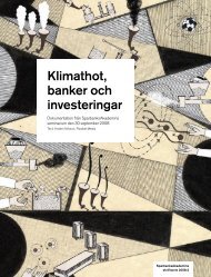
Figure 1. The total energy use for the whole system in a number of scenarios 

Base 

Medium transports 

Medium transports + passenger car 

Long transports 

Natural gas 

Saved wood used as fuel 

Short timeperspective for landfills 

Landfills as carbon sinks 

Plastics replace impregnated wood 

3,0E+09 

2,5E+09 

2,0E+09 

kg CO2-eq./total amount of solid waste 

1,5E+09 

1,0E+09 

5,0E+08 

0,0E+00 

-5,0E+08 

-1,0E+09 

Recycling 

Incineration 

Landfilling 



-1,5E+09 

-2,0E+09 

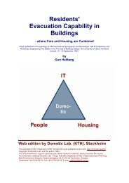
Figure 2. Contribution to global warming from the whole system in different scenarios. 

To summarise some of the overall conclusions it can be noted that recycling of paper and 

plastic materials are in general favourable according to our study with regard to overall 

energy use, emissions of greenhouse gases and the total weighted results. These results are 

fairly robust. When looking at total energy use and emissions of greenhouse gases, recycling 

is the preferred strategy in all scenarios for the whole system, i.e. when all the studied waste

fractions are included. In Figures. 1 and 2 the results from several scenarios are shown 

compared to the base scenario. In the scenario “medium transports” the transport distances are 

increased compared to the base scenario and passenger cars are also assumed to be used in 

one scenario. In the scenario “long transports”, transportation distances are further increased 

compared to the “medium transports” scenario. In the scenario “natural gas”, it is assumed 

that the heat from incineration of waste and gas from digestion and landfilling replaces heat 

from incineration of natural gas. This is a change from the base scenario where it is assumed 

that the competing heat source is forest residues. In the scenario “saved wood used as fuel” it 

is assumed that the wood that is “saved” by recycling of paper materials is used as a fuel for 

heat production replacing natural gas. Such a scenario can correspond to a situation where 

there is increased competition for biomass. In the base scenario, emissions from landfills are 

considered for a hypothetical infinite time period. In the scenario “Short time perspective for 

landfills” this is changed. Also in the scenario “landfills as carbon sinks” only a short time 

perspective is considered and landfills are modelled as carbon traps for nondegraded 

biological materials. In the scenario, “Plastics replace impregnated wood” it is assumed that 

recycled plastics replace impregnated wood as palisades. This is a change from the base 

scenario where it is assumed that recycled paper and plastic materials replace the same 

materials produced from virgin raw materials. 

One exception to the general results is plastics when they are recycled and replace 

impregnated wood. In this case recycling of plastics is less favourable than incineration with 

respect to energy use and emissions of greenhouse gases although the difference is rather 

small. However, recycling may still be favourable with respect to toxicological impacts, and 

our results still show a benefit for recycling with regard to the total weighted results. 

Incineration is in general favourable over landfilling according to our study with regard to 

overall energy use, emissions of gases contributing to global warming and the total weighted 

results. There are however some aspects which may influence this ranking. If longer 

transportation distances are demanded in the incineration case, especially by passenger cars, 

landfilling can become more favourable than incineration. The modelling of landfills can also 

have a decisive influence. If shorter time periods are used, in the order of a century, 

landfilling is favoured and may become a preferable option over incineration. 

LCAs can be used to test the waste hierarchy and identify situations where the hierarchy is not 

valid. Our results suggest however that the waste hierarchy is valid as a rule of thumb. The 

results presented here can be used as a basis for policy decisions as well as strategic decisions 

on waste management systems.

Life Cycle Assessments of Energy from Solid Waste 

PREFACE 

ABSTRACT 

SUMMARY 

CONTENTS 

ABBREVIATIONS 

1 INTRODUCTION 9 

2 METHODOLOGY 12 

3 SCENARIOS AND MAJOR ASSUMPTIONS 30 

4 HOUSEHOLD WASTE COMPOSITION 40 

5. PROCESSES 46 

6 IMPACT ASSESSMENT 75 

7 RESULTS AND DISCUSSION 87 

8. DISCUSSION AND OVERALL CONCLUSIONS 151 

REFERENCES 161 

APPENDIX 1

Contents 

PREFACE 

ABSTRACT 

SUMMARY 

CONTENTS 

ABBREVIATIONS 

1 INTRODUCTION 9 

1.1 BACKGROUND 9 

1.2 LIFE CYCLE ASSESSMENT 10 

1.3 AIM AND SCOPE OF PRESENT STUDY 11 

1.4 SOME GUIDANCE TO THE READER 11 

2 METHODOLOGY 12 

2.1 GENERAL LCA METHODOLOGY 12 

2.1.1 Introduction 12 

2.1.2 Goal and scope definition 13 

2.1.3 Life cycle inventory analysis 14 

2.1.4 Life cycle impact assessment 15 

2.1.5 Interpretation 17 

2.2 LCA METHODOLOGY AND INTEGRATED SOLID WASTE MANAGEMENT 17 

2.2.1 Upstream and downstream system boundaries 17 

2.2.2 Open-loop recycling 18 

2.2.3 Multi-input allocation 20 

2.2.4 Time aspects 20 

2.2.5 Landfills as carbon sinks 21 

2.2.6 Life cycle impact assessment of integrated solid waste management systems 22 

2.3 SCOPE AND METHODOLOGICAL CHOICES MADE IN THIS STUDY 23 

2.3.1 Functional unit 23 

2.3.2 Specification of the goal 23 

2.3.3 Waste materials, treatment methods and the use of scenarios 23 

2.3.4 System boundaries 24 

2.3.5 Open-loop recycling 25 

2.3.6 Time aspects in the case of landfills 25 

2.3.7 Landfills as a carbon sink 26 

2.3.8 Life Cycle Impact Assessment 26 

2.3.9 Data quality and uncertainty 27 

2.4 THE LCA-MODEL IN SIMA PRO 4.0 28 

2.4.1 Methodology and inventory 28 

2.4.2 Impact assessment 29 

2.4.3 Result presentation 29 

3 SCENARIOS AND MAJOR ASSUMPTIONS 30 

3.1 INTRODUCTION 30 

3.2 ELECTRICITY PRODUCTION 30 

3.3 HEAT PRODUCTION 31 

3.3.1 Heat source 31 

3.3.2 Ashes 32 

3.3.3 Forest saved when recycling paper products 32 

3.4 TRANSPORT 32 

Recycling 33 

Digestion and Composting 34 

Incineration 34 

2

Landfill 35 

3.5 LANDFILL MODELLING 36 

3.5.1 Scenario Surveyable Time period (ST) 36 

3.5.2 Scenario ST + Carbon Sink 36 

3.6 SCENARIO PLASTIC PALISADE 37 

3.7 QUALITATIVE DISCUSSIONS 37 

3.8 ADDITIONAL TIME PERSPECTIVES ON GLOBAL WARMING 37 

3.9 SUMMARY OF THE SCENARIOS 37 

3.9.1 Base Scenario 37 

3.9.2 Medium transports scenario 38 

3.9.3 Long transports scenario 38 

3.9.4 Medium transport plus transport by passenger car 38 

3.9.5 Natural gas scenario 38 

3.9.6 Saved forest scenario 38 

3.9.7 Surveyable time period scenario 38 

3.9.8 ST + Carbon sink scenario 38 

3.9.9 Plastic palisade scenario 38 

3.9.10 Excluding metals in ashes from biofuels scenario 38 

3.9.11 Qualitative discussion on degree of efficiency for incineration plants 38 

3.9.12 Qualitative discussion on characterisation of metals 38 

3.9.13 Additional time perspectives on global warming 39 

4 HOUSEHOLD WASTE COMPOSITION 40 


4.2 AVERAGE HOUSEHOLD WASTE COMPOSITION 40 

4.2.1 Composition of waste fractions 41 

Food waste 43 

Newspaper 43 

Corrugated cardboard 44 

Mixed cardboard 44 

Plastics 44 

5. PROCESSES 46 


5.2 RECYCLING 46 

5.2.1 General description 46 

5.2.2 Newspaper 47 

Recycling 47 

Virgin production 49 

5.2.3 Corrugated cardboard 49 

Recycling 49 


5.2.4 Mixed cardboard 50 

Recycling 50 


5.2.5 PE 51 

Recycling 51 


5.2.6 PET 52 

Recycling 52 


5.2.7 PVC, PS and PP 54 

Recycling 54 


5.2.8 Saved forest from paper recycling 55 

5.2.9 Plastic palisade 55 

Recycling of mixed plastic waste into palisades 55 

Virgin production of palisade from wood 56 

5.2.10 Composition of mixed plastics, wood and impregnated wood 57 

5.3 ANAEROBIC DIGESTION 57 


Energy consumption 59 

3

Nutrients content in digestion residue 59 

5.3.2 Transport and spreading of residues from anaerobic digestion and composting 59 

5.3.3 Avoided production of fertilisers, energy and fuel 60 

Nitrogen and phosphorus-fertilisers 60 

Energy and fuel 60 

5.4 COMPOSTING 61 


5.4.2 The composting process 61 

Energy consumption 62 

Air and water emissions 62 

Content of nutrients in the compost residue 63 

5.4.3 Transport and spreading of residues from composting 63 

5.4.4 Avoided production of nitrogen- and phosphorus fertilisers 63 

5.5 INCINERATION 63 


5.5.2 The incineration model 63 

5.5.3 Allocations and system boundaries 65 

5.5.4 Material specific data for incineration 65 

5.6 LANDFILLING 67 


5.6.2 The landfill model 67 

Household waste 67 

Sludge 68 

Landfill fires 69 

Leachate treatment 69 

Landfill gas 70 

Transports and energy 70 

5.6.3 Landfill as carbon sink 70 

5.6.4 Other landfilling options 71 

Biocells 71 

5.7 ELECTRICITY PRODUCTION 71 

5.7.1 Electricity from hard coal 71 

5.7.2 Exceptions 72 

5.8 TRANSPORTS 72 


5.8.2 Trucks 72 

5.8.3 Garbage truck 72 

5.8.4 Passenger car 73 

5.9 HEAT PRODUCTION 73 


5.9.2 Residues of timber felling 73 

5.9.3 Natural gas 74 

5.9.4 Heating oil 74 

6 IMPACT ASSESSMENT 75 


6.2 CHARACTERISATION METHODS 75 

6.2.1 Energy 75 

6.2.2 Abiotic resources 75 

6.2.3 Non-treated waste 75 

6.2.4 Global warming 75 

6.2.5 Stratospheric ozone depletion 76 

6.2.6 Photo-oxidant formation 76 

6.2.7 Acidification (excluding SO x and NO x ) 76 

6.2.8 Aquatic eutrophication (excluding NO x ) 77 

6.2.9 NH 3 77 

6.2.10 Toxicological effects 77 

USES-LCA 77 

EDIP 79 

6.2.11 Undefined substances 80 

6.3 WEIGHTING USING ECOTAX 98 81 

Abiotic resources 81 

4

Non-treated waste 82 

Global warming 82 

Stratospheric ozone depletion 82 

Photo-oxidant formation 82 

Acidification (excluding SO x and NO x ) 82 

Aquatic eutrophication (excluding NO x ) 82 

SO x 82 

NO x 82 

NH 3 82 

Toxicological effects 83 

6.4 ECO-INDICATOR 99 85 

6.4.1 Human health 85 

6.4.2 Ecosystem quality 85 


6.4.4 Additions 86 

7 RESULTS AND DISCUSSION 87 


7.2 RESULTS BASE SCENARIO 88 

7.2.1 Total Energy 88 

7.2.2 Non-renewable energy 90 


7.2.4 Non-treated waste 90 


7.2.6 Photo-oxidant formation 93 

7.2.7 Acidification (excluding SO x and NO x ) 93 

7.2.8 Aquatic eutrophication (excluding NO x ) 93 

7.2.9 NO x 94 

7.2.10 SO x 94 

7.2.11 Terrestrial eutrophication from NH 3 94 


Ecotoxicity 95 

Toxicological effects on human health 96 

7.2.13 Undefined substances 98 

7.2.14 Total weighted results 98 

7.2.15 Eco-indicator 99 99 

7.2.16 Summary 101 

7.3 RESULTS SCENARIO MEDIUM TRANSPORTS 101 

7.3.1 Energy, abiotic resources and non-treated waste 102 

7.3.2 Non-toxicological impacts 103 



7.3.5 Summary 106 

7.4 RESULTS SCENARIO LONG TRANSPORTS 106 





7.4.5 Summary 111 

7.5 RESULTS SCENARIO MEDIUM TRANSPORTS AND TRANSPORTS BY PASSENGER CAR 111 





7.5.5 Summary 118 

7.6 RESULTS SCENARIO NATURAL GAS FOR HEAT PRODUCTION 118 


7.6.2 Energy, abitoic resources and non-treated waste 119 


7.6.4 Toxicological impacts 122 


5

7.6.6 Summary 125 

7.7 RESULTS SCENARIO SAVED FOREST USED FOR HEAT PRODUCTION 126 






7.7.6 Summary 131 

7.8 RESULTS SCENARIO SURVEYABLE TIME PERIOD (ST) 131 





7.8.5 Summary 137 

7.9 RESULTS SCENARIO ST + CARBON SINK 137 



7.9.3 Summary 139 

7.10 RESULTS SCENARIO PLASTIC PALISADE 140 






7.10.6 Summary 141 

7.11 RESULTS SCENARIO EXCLUDING METALS IN ASHES FROM BIOFUELS 142 




7.11.4 Summary 145 

7.12 RESULTS QUALITATIVE DISCUSSIONS 146 

7.12.1 Incineration plant, degree of efficiency 146 

7.12.2 Characterisation of metals as a group 146 

7.13 RESULTS ADDITIONAL TIME PERSPECTIVES ON GLOBAL WARMING 147 



8. DISCUSSION AND OVERALL CONCLUSIONS 151 

8.1 SUMMARY OF SOME OF THE RESULTS 151 


8.1.2 Energy use 151 


8.1.4 Total weighted result 155 

8.1.5 Food waste 155 

8.2 RESULTS COMPARED TO NATIONAL REFERENCES 156 

8.3 IMPACT ASSESSMENT METHODS 157 

8.4 LIMITATIONS AND NEED FOR FURTHER RESEARCH 158 

8.5 SUMMARISED CONCLUSIONS 159 

8.6 POLICY IMPLICATIONS 159 

REFERENCES 161 

APPENDIX 1 

SOURCES FOR DATA ON ADDITIVES, ENERGY AND TRANSPORTS 

6

Abbreviations 

AOX 

Adsorbable halogenated organic material 

BOD 

Biological oxygen demand 

CFB 

Circulating fluidised bed 

CHX 

Volatile halogenated hydrocarbons 

COD 

Chemical oxygen demand 

DALY 

Disability adjusted life years 

DEHP 

Dietyl-hexyl-ftalat 

DOC 

Dissolved organic compounds 

DOM 

Dioktyl-tin-maliat 

EDIP 

Environmental design of industrial products 

EIA 

Environmental Impact Assessment 

GWP 

Global warming potential 

HBFC 

Bromine-containing halocarbons 

HDO 

Bis-(N-cyclohexyldiazenium-dioxy) 

HDPE 

High density polyethylene 

HHV 

Higher heating value 

LCA 

Life Cycle Assessment 

LCIA 

Life Cycle Impact Assessment 

LHV 

Lower heating value 

LPG 

Liquefied petroleum gas 

NMVOC 

Non-methane volatile organic compounds 

NT waste 

Non-treated waste 

ODP 

Ozone depletion potential 

PAF 

Potentially affected fraction 

PAH 

Polyaromatic hydrocarbons 

PCB 

Polychlorinated biphenyls 

PET 

Polytethyleneterephtalate 

POCP 

Photochemical ozone creation potential 

PP 

Polypropylene 

PS 

Polystyrene 

PVC 

Poly(vinyl chloride) 

RA 

Risk Analysis 

Ra 

Required acreage 

RT 

Remaining time period 

SFA 

Substance Flow Analysis 

SNCR 

Selective non-catalytic reduction 

SP Sima Pro 4.0 

SPOLD 

Society for Promotion of Life Cycle Assessment Development 

ST 

Surveyable time period 

TMP 

Thermo mechanical pulp 

TMT 15 

Trimercapto-s-triazine-tri-sodium-salt 

TOC 

Total organic carbon 

TS 

Total solids 

7

USES 

VOC 

YLD 

YLL 

Uniform system for the evaluation of substances 

Volatile organic compounds 

Numbers of years lived disabled 

Numbers of years of life lost 

8

1 Introduction 

1.1 Background 

We live in a changing world. In many countries both energy systems and waste management 

systems are currently undergoing changes. One driving force for these changes is the threat of 

global climate change caused by increasing concentrations of carbon dioxide (CO 2 ), methane 

(CH 4 ) and other greenhouse gases. This threat has lead the global society to sign the Kyoto 

protocol 1997 which simplistically states that the developed countries should reduce their 

emissions by 5 % until the year 2010 compared to 1990 (SOU 2000). These reductions will 

however probably be followed by more stringent reductions. For example, a recent 

parliamentary committee in Sweden (SOU 2000) has suggested that the Swedish emissions of 

greenhouse gases should be reduced by 2 % until the year 2010 and by 50 % until the year 

2050 with further reductions after that (SOU 2000). In Sweden the energy system is being 

changed, not only because of the threat of global climate change but also because of the 

planned phase out of nuclear power, deregulation of the electricity markets and following 

increased possibilities for import and export of power between different markets among other 

things. 

One way of reducing emissions of greenhouse gases from the energy system is to reduce the 

use of fossil fuels. In many countries there is currently ongoing discussions on how to reduce 

the use of fossil fuels and increase the use of renewable fuels. Waste is sometimes regarded as 

a renewable fuel. Policies on waste management systems should therefore be considered 

together with policies on energy systems. Another way of reducing emissions of greenhouse 

gases is to reduce emissions of methane (CH 4 ) from degradation of organic materials in 

landfills. This is one reason for the policy in many countries to reduce landfilling of organic 

materials. 

The waste management systems in Sweden are affected by the recent decision on a landfill tax 

and the decision to stop landfilling of organic waste after the year 2005. Investments must 

therefore be made in alternative management options for the waste that is currently being 

landfilled. Before making such investments it is important to examine the consequences of 

different choices. This study is intended as one basis for strategic decisions regarding waste 

management energy policies. 

A waste hierarchy is often suggested and used in waste policy making. Different versions of 

the hierarchy exist but in most cases it suggests the following order: 

1. Reduce the amount of waste 

2. Reuse 

3. Recycle materials 

4. Incinerate with heat recovery 

5. Landfill 

The first priority, to reduce the amount of waste, is in general accepted. However, the 

remaining waste needs to be taken care of as efficiently as possible. Different options for 

taking care of the remaining waste is the topic of this study. 

The hierarchy after the top priority is often contested and discussions on waste policy are in 

many countries intense. Especially the order between recycling and incineration is often 

9

discussed. Another question is where to place biological treatments such as anaerobic 

digestion and composting in the hierarchy. One of the aims of this study is to evaluate the 

waste hierarchy. 

1.2 Life Cycle Assessment 

It is interesting to note that the changes in both energy and waste management systems to a 

large extent are driven by environmental considerations and arguments. It is therefore of 

importance when making decisions on policies as well as on investments to consider the 

environmental implications. A large number of methods and tools for describing 

environmental aspects have been developed which can be used in different types of decision 

contexts (Moberg et al. 1999). In this study we are using Life Cycle Assessment for 

comparing different alternative waste treatment strategies. 

Life Cycle Assessment (LCA) studies the environmental aspects and potential impacts 

throughout a product’s life (i.e. from cradle to grave) from raw material acquisition through 

production, use and disposal (ISO 1997). The LCA methodology is described in detail in 

chapter 2. Here it is of interest to note two important aspects of LCA, which makes the tool 

unique. The first is the focus on products, or rather functions that products provide. Products 

can include not only material products but also service functions, for example taking care of a 

certain amount of solid waste or producing a certain amount of heat or electricity. This is an 

appropriate perspective when comparing different options for waste treatment or methods for 

generating heat and electricity. 

The second aspect of LCA is the cradle-to-grave perspective. When comparing different 

products fulfilling a similar function it can be important to consider the complete life cycle. 

This is because environmental impacts and benefits may occur at different phases of the lifecycle. 

Here are two examples of relevance for both energy and waste management policies, 

which illustrate the need to consider wide enough system boundaries in a reasonably 

standardised procedure (Finnveden 1999a): 

• Ethanol can be produced from paper fractions of solid waste. The ethanol can be used as a 

fuel for buses with, in general, less emissions of pollutants than for example diesel fuels 

during the use phase. However, the production of ethanol is energy demanding and if 

fossil fuels are used for the production, the total result of the complete life cycle is not in 

favour of the ethanol alternative (Finnveden et al. 1994). 

• Recycling, incineration and landfilling of waste material were compared in a recent costbenefit 

analysis by Bruvoll (Bruvoll 1998). However, the system boundaries of the study 

were too narrow for a fair comparison. For example, increased transports of recycled 

materials were included but not decreased transports of virgin material which was 

assumed to be replaced by the recycled material (Finnveden 1998). 

LCA is currently being used in several countries to evaluate different strategies for Integrated 

Waste Management, e.g. Finnveden and Huppes (1995), White et al. (1995), Denison (1996), 

Aumônier and Coleman (1997), Sundberg et al. (1998), Hassan et al. (1999), Tukker (1999a, 

b), Weitz et al. (1999), Clift et al. (2000), Sundqvist et al. (2000) and to evaluate treatment 

options for specific waste fractions, e.g. paper Finnveden and Ekvall (1998), Ekvall and 

Finnveden (2000c) and plastics Heyde and Kremer (1999). 

10

1.3 Aim and scope of present study 





results. The results are intended to be used by decision-makers in local, regional and national 

authorities and industries as one basis for decisions on strategies and policies for waste 

management and investments for new waste treatment facilities. Some aspects of the scope 

are: 

• The focus is on Swedish conditions, but it is expected that much of the results will be of 

interest also for other countries 

• The intended use is for assessing effects of different strategic choices made today or the 

coming years. These effects will however prevail for decades since the lifetime of the 

investments will be comparatively long. The time frame of the treatment systems is 

therefore extended from the current situation to several decades into the future. 

• Included in the study are fractions of municipal solid waste, which are combustible and 

recyclable or compostable. 

• The focus is on energy use and climate change although other impact categories such as 

acidification, eutrophication, photo-oxidant formation and human and ecotoxicological 

impacts are also considered. 

The scope of the study is further defined in section 2.3. 

1.4 Some guidance to the reader 

In chapter 2, LCA methodology is presented and discussed. Section 2.1 is a general 

presentation of LCA methodology and can be skipped by those familiar to LCA. Section 2.2 

contains a discussion on some methodological issues of special relevance for LCA of waste 

management systems. Section 2.3 includes a presentation of methodological choices made in 

this study and it is probably of importance for any reader who wants to have something more 

than just a quick feeling of the report. The methodological choices made for the impact 

assessment are partly described in section 2.3 and in more detail in chapter 6. Section 2.4 

contains a description of the LCA software programme that is used. 

Chapter 3 contains a description of the scenarios used in this study (one base scenario and 

several “what-if scenarios”) and some major assumptions. At the end of the chapter there is a 

summary which may be enough to read for some readers of this report. 

Chapter 4 contains detailed descriptions of the waste materials studied and the amounts of 

them. Chapter 5 contains detailed descriptions of the processes included in the study. Many 

readers are probably not interested in all the details of these chapters. 

Chapter 7 contains a fairly detailed presentation of the results of all scenarios. Many readers 

may not be interested in all the details of this chapter and may look at some of the tables and 

go directly to chapter 8, using chapter 7 as a reference for aspects of particular interest. 

Appendix 1 includes data on additives, energy and transports used in this study, which are 

mentioned in chapter 5 but not described in detail there. Appendix 1 is included in this report. 

Appendix 2-7 are available as separate reports, see preface for details on contents. 

11

2 Methodology 

2.1 General LCA methodology 

2.1.1 Introduction 

This section is devoted to a brief introduction to life cycle assessment. The presentation is 

based on UNEP (1996) in addition to a number of LCA references such as Lindfors et al. 

(1995), Udo de Haes (1996), Frischknecht (1997), ISO (1997), Weidema (1998), ISO (1999), 

Johansson (1999), Udo de Haes et al. (1999a), Udo de Haes et al. (1999b), Clift et al. (2000) 

and Finnveden (000a) 

In a life cycle assessment (LCA) the environmental impacts of a product or service are 

investigated throughout its whole life cycle. This is done by compiling an inventory of 

relevant inputs and outputs of a system (inventory analysis), evaluating the potential impacts 

of those inputs and outputs (impact assessment), and interpreting the results (interpretation) in 

relation to the objectives of the study (defined in the scope and goal definition in the 

beginning of the study) (ISO 1997). A standardised framework on how to perform an LCA is 

provided by the International Standards Organisation (ISO 1997). According to this 

framework a life cycle assessment consists of four different, but interrelated phases, as 

illustrated in Figure 2.1. The different phases of LCA are described below, mainly based on 

the ISO-standard. 

The framework for life cycle assessment 

Goal and scope 

definition 

Life cycle inventory 

analysis 

Interpretation 

Direct applications: 

• Product development 

and improvement 

• Strategic planning 

• Public policy making 

• Marketing 

• Other 

Life cycle impact 

assessment 

Figure 2.1. The phases of a life cycle assessment (modified from ISO (1997). 

12

The LCA shall cover the use of material and energy as well as all emissions made by the 

product system in a cradle-to-grave perspective. As defined in the Nordic Guidelines on Life 

Cycle Assessment (Lindfors et al. 1995), this means that the product system is followed from 

the extraction and processing of raw material, through manufacturing, distribution, use, reuse, 

maintenance, recycling to final disposal, including all transports involved. Quantitative or 

qualitative information on emissions made, and material and energy used in all those phases 

are gathered and processed so that an assessment can be made on the total impact on the 

environment and on the resource base. An LCA does not involve economic or social impacts 

(Lindfors et al. 1995). The general categories of environmental impacts needing attention 

include resource use, human health and ecological considerations (ISO 1997). 

An LCA study can be a valuable support for various kinds of environmental decisions, such 

as the design or improvement of products and processes, the development of business plans, 

the setting of ecolabeling criteria, the developing of policy strategies, and when making 

purchasing decisions. 

The focus of an LCA may be either on a product, such as a car, or on a function, such as the 

transportation of one person from point A to point B. The LCA is always based on a so called 

functional unit. The functional unit is a reference unit for quantifying the performance of a 

product system. When for example comparing washing up by hand with using a dishwasher, 

the functional unit could be the washing-up needed by a four-person household for one year. 

This approach gives a relative indication of what potential damage the product system might 

give rise to, and an LCA can thus never tell what actual damage that is going to occur in the 

environment. 

There are several other environmental decision tools available addressing different aspects, 

for example risk analysis (RA) for hazardous chemicals and activities; environmental impact 

assessment (EIA) for new activities; and substance flow analysis (SFA) for substances. The 

different techniques should not be seen as competitive, but rather as complementary. (For a 

comparison of different environmental analysis tools, se e.g. Moberg et al. (1999). 

Performing an LCA is an iterative process, where information revealed during the course of 

the study may impose a revision of earlier steps. As, for example, the most important 

processes are identified, the scope of the study may have to be altered. The process is repeated 

until the goal of the study is met. 

2.1.2 Goal and scope definition 

In the goal of an LCA study the intended application and the reasons for carrying out the 

study shall be clearly stated. It shall also be defined to whom the results produced are 

intended to be communicated. 

The goal set in turn defines the scope needed for the study in order to meet that goal. In the 

scope the functions of the system under study are specified, and the functional unit, on which 

the investigation shall be based, is determined. 

It is unfeasible to cover absolutely every aspect linked to the life of a product. Therefore the 

system boundaries have to be determined. That is, a decision concerning which unit processes 

to be included within the LCA has to be made. The data quality required to fulfil the goal of 

the study is also specified in the scope, addressing issues like time related coverage, 

13

geographical coverage, and consistency and reproducibility of the methods used. In 

comparative studies any differences between systems, regarding functional unit and 

methodological considerations shall be identified and reported. 

The goals of an LCA can be analysed in several dimensions. A first fundamental dimension is 

concerned with whether the study is change-oriented (prospective) or descriptive 

(retrospective) (Frischknecht 1997, Baumann 1998, Weidema 1998). If the study is changeoriented 

it analyses the consequences of a choice; ideally the data used should reflect the 

actual changes taking place, and may depend on the scale of the change and the time over 

which it occurs. With regard to time, a distinction can be made between a very short time 

frame (less than a year), short (years), long (decades) or very long (centuries). Studies which 

are not change-oriented may be called environmental reports. In such studies the appropriate 

data should reflect what was actually happening in the system (Clift et al. 2000). 

For a change-oriented, prospective study, the ideal data is in general some sort of marginal 

data reflecting the actual change (Tillman 1999, Weidema et al. 1999a). A procedure for 

identification of the marginal has been suggested by (Weidema et al. 1999a). If the time 

perspective is long (decades) it is in general changes in the base-load marginal that are of 

relevance. The long-term base-load marginal is determined by several aspects, e.g. if the total 

market is increasing or decreasing and if there are any aspects constraining the use of a 

specific technology. If the total market is increasing, new investments will be made. The baseload 

marginal technology is the technology in which new investments are made. This is the 

preferred, unconstrained technology (Weidema et al. 1999a). If the market is decreasing, 

production capacity will be decreased and the marginal technology is the technology that will 

be decreased. This is the least preferred technology (Weidema et al. 1999a). 

2.1.3 Life cycle inventory analysis 

The inventory analysis is the phase when data is collected and calculations are made in order 

to specify relevant inputs to and outputs from the product system. This work can be divided 

into four different substeps (UNEP 1996) which in practise are performed simultaneously. 

First, all processes involved in the life cycle of the product system have to be identified. 

Ultimately, all processes start with the extraction of raw materials and energy from the 

environment. After the transformation by various economic processes, all those inputs from 

the environment will eventually re-enter the environment as emissions to air, water and land. 

To clarify these often complex processes, a process flow chart is constructed. 

Secondly, the data on each process is collected. This is the most time consuming and difficult 

task in performing an LCA. Data can be obtained from scientific literature, from published 

data files used by LCA practitioners, from industry and from government records. The data 

used should preferably be quantitative, but when it proves too difficult to find quantitative 

data a qualitative estimation can be made instead. 

The third step is to define once again the system boundaries. This time it can be done more 

carefully with the information from the system flow chart and the collected data. This will 

give the LCA study a more manageable size, as processes that fall outside these boundaries 

can be left out. Boundaries need to be set separating the product system from the 

environment, from other product systems and from processes not taken into account in the 

product system (UNEP 1996). The system boundary between the studied product system and 

14

other product system boundaries leads to so called allocation problems, which are further 

discussed below. 

Finally, the inputs and outputs from all processes are adjusted to relate to the functional unit. 

Aggregation of all data, through addition, then results in an inventory table. In the inventory 

table all economic inputs and outputs will have been translated into environmental inputs and 

outputs, in terms of resource extraction and emissions. 

2.1.4 Life cycle impact assessment 

As the inventory table often contains a vast number of figures, that are difficult to interpret 

intuitively, the need for a more formalised evaluation arises. The inventory table constitutes 

the input to the life cycle impact assessment (LCIA). According to the ISO-standard (ISO 

1999), the LCIA is a phase of the LCA aimed at understanding and evaluating the magnitude 

and significance of the potential environmental impacts of a product system. It is divided into 

several elements; some are described as mandatory in an LCIA and some as optional. 

The first mandatory element is a selection of a manageable number of impact categories of 

resource use and environmental impacts, indicators for the categories and models to quantify 

the contributions of different inputs and emissions to the impact categories. As an example of 

impact categories that may be discussed in an LCIA, Table 2.1 presents a default list 

suggested by the SETAC-Europe working group on LCIA (Udo de Haes 1996). In practice 

however, a shorter list of impacts are normally included in current LCAs (Finnveden 2000a). 

The second mandatory element (classification) is an assignment of the inventory data to the 

impact categories. The third mandatory element (characterisation) is a quantification of the 

contributions to the chosen impacts from the product system. 

Table 2.1. Default list of impact categories for life cycle impact assessment (Udo de Haes 1996). 

Input related categories 

1. Abiotic resources (deposits, funds, flows)* 

2. Biotic resources (funds) 

3. Land 

Output related categories 

4. Global warming 

5. Depletion of stratospheric ozone 

6. Human toxicological impacts 

7. Ecotoxicological impacts 

8. Photo-oxidant formation 

9. Acidification 

10. Eutrophication (incl. BOD and heat) 

11. Odour 

12. Noise 

13. Radiation 

14. Casualties 

Pro memoria: Flows not followed to the system boundary 

Input related 

Output related 

*Deposits are resources which can only be depleted, with no renewability within the timeframe considered 

(examples include mineral ores and fossil fuels). Funds are resources which are intrinsically renewable but 

which can be depleted (examples include wood and fish). Flows are resources which can be deflected and used 

but not depleted (examples include wind and solar radiation). 

There are also several optional elements which can be used depending on the goal and scope 

of the LCA (ISO 1999). Normalisation relates the magnitude of the impacts in the different 

categories to reference values; an example of a reference value is the total contribution to an 

impact category by a nation. Grouping includes sorting and possibly ranking of the 

indicators. Weighting aims at converting and possibly aggregating results across impact 

categories resulting in a single result, sometimes with a monetary measure. The final element 

is a data quality analysis, which is described as mandatory in comparative assertions. 

15

Weighting is and has always been a controversial issue, in large part because this element 

requires social, political and ethical values e.g. Finnveden (1997) whereas the preceding steps 

are based on more traditional natural sciences. Another aspect is that most of the presently 

available weighting methods for LCA seem to have significant drawbacks (Finnveden 1999b). 

The controversy around Weighting as an element in the analysis and weighting methods is 

also illustrated by the ISO standard, which states that weighting shall not be used in 

“comparative assertions disclosed to the public”(ISO 1999). 

It is sometimes noted, e.g. in the ISO standard (ISO 1999), that the methodological and 

scientific framework for LCIA is still being developed. Methods for different impact 

categories are in different stages of development. Work is currently ongoing to develop a set 

of best available practices regarding impact categories and category indicators (Udo de Haes 

et al. 1999a, Udo de Haes et al. 1999b). 

The relations between the Inventory Table, Classification and Characterisation and Weighting 

are illustrated in Figure 2.2. 

CLASSIFICATION AND CHARACTERISATION WEIGHTING 

............. 

Inventory 

table 

CO 2 

CH 4 

CFC 

.... 

GLOBAL WARMING 

SO 2 

NO x 

NH 4 

.... 

ACIDFICATION 

Environmental 

index 

NO x 

NH 4 

P 

CO 

D 

EUTROPHICATION 

............... 

Figure 2.2. Some of the steps involved in the life cycle impact assessment (modified from UNEP (1996). 

16

2.1.5 Interpretation 

In the interpretation phase of LCA the findings from the inventory analysis and the impact 

assessment are combined together in order to reach conclusions and recommendations, 

consistent with the goal and scope of the study (ISO 1997). This phase may also involve the 

reviewing and revising of the goal and scope, as well as the nature and quality of the data 

collected. 

2.2 LCA Methodology and Integrated Solid Waste Management 

The general LCA methodology has been described above. Essentially the same methodology 

can be applied when applied to waste management systems although different aspects of the 

methodology may come into focus. It is also important to notice that although improvements 

have been made to LCA methodology, there are still a number of unresolved issues, which 

need further attention (Udo de Haes and Wrisberg 1997). Here, some methodological aspects 

of relevance for LCAs on waste management systems will be discussed. It is suggested that 

many of these aspects are of relevance also for other types of systems engineering models of 

waste management systems (Finnveden 1999c). This section is largely based on previous 

methodological publications (Finnveden 1999c, Clift et al. 2000, Ekvall and Finnveden 

2000b, Finnveden 2000b). Aspects that will be discussed include: Upstream and downstream 

system boundaries, Open-loop recycling allocation, Multi-input allocation, Time especially in 

relation to landfills, Landfills as a carbon sink, and Life cycle impact assessment. 

2.2.1 Upstream and downstream system boundaries 

A key aspect of LCA is that the system should be modelled in such a manner so that inputs to 

and outputs from the system are followed from the “cradle to the grave”, which means that the 

inputs should be flows that are drawn from the environment without human transformation, 

and outputs should be flows that are discarded to the environment without subsequent human 

transformations (ISO 1997). In LCAs of waste management systems, this is typically not 

done. Instead, the inputs are often solid waste as they appear, e.g. from households. This is, 

however, still compatible with the LCA definition, if the same inflow appears in all systems 

which are to be compared. This is because those parts of the systems, which are identical in 

all systems that are compared, can be disregarded. The upstream system boundary may, 

however, have to be changed, if one of the systems to be compared produce more or less 

waste than the others. In this situation the system inputs are no longer identical, and in 

principle the system boundary should be moved and upstream activities be included, at least 

those parts which differ between different systems. This may in practise prove to be very 

difficult and therefore not done. In that case it should, however, be carefully noted that the 

impacts of the system which produces less waste is overestimated compared to the others. 

A similar situation may occur for the downstream system boundary when materials or energy 

are recycled into new products. In LCAs of waste management systems, products from 

recycling are normally not followed to the “grave” and neither are the products, which are 

replaced by the products from recycling. Again this is compatible with the LCA definition, if 

the products are “identical” in all systems which are compared. In these cases the products 

can be disregarded. “Identical” does not mean that they have to be exactly identical in all 

aspects. It is enough if they are providing a comparable function to the user, and if they have 

the same environmental impacts. If the products are not providing comparable functions, they 

cannot replace each other. If the products do not have the same environmental impacts, at 

least the difference should be included in the LCA. 

17

2.2.2 Open-loop recycling 

Open-loop recycling takes place when a product is recycled after its use into another product. 

This can be a problem since the system boundary between products 1 and 2 is not clear-cut. 

Open-loop recycling has been much discussed in the LCA literature e.g. Huppes and 

Schneider (1994), Finnveden and Huppes (1995), Lindfors et al. (1995), Udo de Haes and 

Wrisberg (1997), Ekvall (1999) and Ekvall and Finnveden (2000b). The problem can be 

solved in two ways: by allocating environmental interventions between the two products and 

study only one of them, or by expanding system boundaries and including both products 

within the system. 

If allocation is to be made, there are three parts of the system that should be allocated between 

the two products (Lindfors et al. 1995): 

1) the recycling system 

2) production of primary material used in both products 

3) disposal of materials used in both products 

Many methods for the allocation have been suggested in the literature and used in case studies 

(Huppes and Schneider 1994, Lindfors et al. 1995, Ekvall 1999). There does not seem to be 

any procedure that proves that any specific method is the “correct” one. Instead arguments are 

usually based on what intuitively seems reasonable or fair. However, such arguments can lead 

to very different conclusions and different allocation procedures can lead to different results 

(Ekvall and Tillman 1997). 

In order to avoid the allocation problem, system boundaries can sometimes be expanded to 

include several functions within the system. An example is the comparison between 

landfilling and incineration of waste. The main function of landfilling is treatment of solid 

waste. (In addition landfill gas is sometimes collected and used, but this aspect is however 

neglected in this methodological discussion). Incineration with heat recovery also treats solid 

waste, but in addition produces heat or electricity, thus providing a second function (Figure 

2.3a). Since the processes provide different functions, it is difficult to directly compare them. 

In the expanded system an alternative method of producing an equivalent amount of heat has 

been added to the landfill system (Figure 2.3.b). It is thus possible to compare the incineration 

system to the combined landfill and heat producing systems. The systems compared are multifunctional 

systems. Another way of presenting the expanded systems is to subtract the heatproducing 

system from the incineration system using an alternative heat-source, as described 

in Figure 2.3.c. Since the same components are included, it is essentially the same systems 

which are presented in Figure 2.3.b and 2.3.c. In the system shown in Figure 2.3.c, so called 

“avoided emissions” will occur and environmental interventions may become negative. 

When using system expansion, several functions are studied at the same time. This is not 

always apparent since the subtracted systems appear as single-functional. When using system 

expansion it is no longer possible to study one function in isolation. This can be seen as an 

advantage since this reflects the real situation. In a situation where different functions cannot 

be chosen independently, it is an advantage if this is reflected in the LCA. For example, if a 

choice is made to incinerate solid waste with heat recovery, it is no longer possible to choose 

another energy source and this is illustrated in the expanded system. Also, from another 

perspective, if solid waste is chosen as the energy source, it is no longer possible to choose 

another treatment method for solid waste. This illustrates that if solid waste is considered as 

18

an energy source, the energy system and waste management system must be considered 

simultaneously. This also implies that the systems will be identical whether the starting point 

is the choice of energy source, or the choice of waste treatment. 

Incineration 

Landfilling 

Functions: Treatment of 

solid waste 

Heat 

Function: Treatment of 

solid waste 

a. 

Incineration 

Landfilling 

+ 

Alternative 

heat source 


solid waste 

Heat 


solid waste 

Heat 

b. 

Incineration 

- 

Alternative 

heat source 

Landfilling 

Functions: Treatment of Heat Heat 

solid waste 

Function: Treatment of 

solid waste 

c. 

Figure 2.3.a. An example of an allocation problem. b. A possible way of avoiding the allocation problem by 

expanding the system boundary. c. An alternative way of presenting the expanded system boundary described in 

figure b. (Finnveden and Ekvall 1998) 

The use of expanded system boundaries to avoid the allocation problem is often 

recommended, for example in the Nordic Guidelines (Lindfors et al. 1995), and the ISOstandard 

(ISO 1998). The ISO-standard has been critically reviewed, but system expansion is 

still generally recommended for change-oriented studies, e.g. Tillman (1999) and Ekvall and 

Finnveden (2000b). There are however some critical questions to consider when using system 

expansion (Ekvall and Tillman 1997, Ekvall and Finnveden 2000b). For example: 

1) What material will the recycled material replace? It is often assumed that the recycled 

material will replace virgin material of the same kind. For example, recycled paper is 

19

often assumed to replace virgin paper. However, in some cases, recycled paper may 

replace another type of recycled paper or another material, e.g. plastic. 

2) If (more or less) waste is incinerated with heat recovery, what is the alternative energy 

source? This question is of interest when comparing incineration with heat recovery with 

other treatment methods. The same applies for other treatment options, anaerobic 

digestion and landfilling with gas collection, where heat may be generated. In the case of 

comparing recycling to incineration of paper packaging material, it has been shown that 

assumptions concerning the alternative energy source can be decisive to the outcome of 

the study (Finnveden and Ekvall 1998, Ekvall and Finnveden 2000c). 

3) Are the demands independent of how the products are produced? It is generally assumed 

in LCAs that the demands for the functions fulfilled by the systems are independent of 

how they are fulfilled (Tillman et al. 1994). The system modelled is thus a simplification 

of the real system. 

4) Are the functional qualities of the products and/or material similar and independent of 

how they are produced? It is often assumed that the recycled material can replace another 

material having similar functional qualities. If the materials are similar, the processes 

downstream may be considered as identical and disregarded in a comparative assessment, 

greatly facilitating the study, as discussed above. 

The answers to these and other questions are likely to depend on the goal of the study as 

briefly discussed in section 2.1.2. Important aspects to consider are for example the time 

frame for the study and what type of decisions might be based on the analysis. 

2.2.3 Multi-input allocation 

One type of allocation problem (the case of open-loop recycling) was discussed above. 

Another type is called the multi-input allocation problem. It occurs when several products are 

inputs to processes, and it focuses on determining which environmental interventions should 

be allocated to which products. One example can be emissions of hydrocarbons with landfill 

gas. Some of these chemicals may be degradation products and some may come from specific 

products in the waste. The question is how the emissions shall be allocated to the different 

products and materials in the waste. Another example concerns emissions of chlorinated 

hydrocarbons from incineration of municipal solid waste. 

The guiding principle for the multi-input allocation problem should be the underlying 

physical, chemical or biological relationships and there is a general agreement in the LCA 

world on this e.g. Finnveden and Huppes (1995), Lindfors et al. (1995) and ISO (1998). The 

question then becomes a scientific/technical question of finding the relevant causalities. This 

in turn may turn out to be dependent on the purpose of the study as briefly discussed above. 

For example, if the relationships between inputs and emissions are non-linear, the scale of 

change should influence the allocation. 

2.2.4 Time aspects 

One important difference between landfilling and most other processes in an LCA is the time 

frame. Emissions from landfills may prevail for a very long time, often thousands of years or 

longer. The potential emissions from landfilling have to be integrated over a certain timeperiod. 

It is important to determine which time period is of interest. There is currently no 

international agreement on this question (Finnveden and Huppes 1995). Using the LCA 

definition as a starting point, it can be argued that emissions should be integrated until 

infinity. In practise however, a shorter time frame (decades and centuries) has usually been 

chosen (see Finnveden (1999c) for a review). The choice of the time period can have a 

20

significant influence on the results for materials that are persistent (e.g. plastics) and for 

substances which are only slowly leaching out, e.g. metals from municipal solid waste and 

ashes (Finnveden 2000b). 

The choice of the time frame is clearly a value choice for the inventory analysis of an LCA. It 

is related to ethical views about impacts on future generations (Finnveden 1997). It is clearly 

a question that deserves more attention. Important aspects to discuss include the possibilities 

and consequences of different choices as well as the ethical discussion, which apparently can 

not be avoided. A similar situation may occur for different parts of the life cycle impact 

assessment. The choice made by the SETAC-Europe working group on Life cycle impact 

assessment is to consider first the infinite time period, then a short time period of 100 years 

and finally if wanted other time periods (Udo de Haes et al. 1999a, Udo de Haes et al. 1999b). 

2.2.5 Landfills as carbon sinks 

When carbon flows in landfills are modelled, a distinction is often made between biotic (from 

renewable sources) and non-biotic carbon (from fossil sources). Common practise is to 

disregard biotic CO 2 -emissions. This can be motivated from different perspectives (Dobson 

1998). One includes an expansion of the system boundary to include also the uptake of the 

CO 2 in the growing tree. This expansion is often done as a thought experiment rather than an 

actual modelling. Another perspective can be the assumption that when biotic resources are 

harvested, new resources are planted which will take up an equivalent amount of CO 2 . Again 

this modelling is normally not done explicitly. Yet another perspective is the assumption that 

if the biotic resources, e.g. trees, had not been harvested, they would have been left in the 

forest and degraded there. This degradation can however be quite slow, and the time frame 

has to be extended to several centuries before all biotic materials have been degraded 

(Zetterberg and Hansén 1998). 

The practise to disregard biotic CO 2 -emissions can lead to erroneous results (Dobson 1998). 

Let us consider an example to illustrate this. Let us compare incineration and landfilling of a 

hypothetical product consisting of only cellulose. When incinerated, nearly 100 % of the 

carbon is emitted as CO 2 . However, in the inventory, this emission is often disregarded as 

noted above. If the product is landfilled, approximately 70 % of the material is expected to be 

degraded and emitted during a short time period, mainly as CO 2 and CH 4 (Finnveden et al. 

1995) (The short time period is here defined as the surveyable time period, which will be 

explained in 2.3.6). Again the emitted CO 2 is normally disregarded, although the CH 4 - 

emissions are noted. During the surveyable time period, 30 % of the carbon is expected to be 

trapped in the landfill. There is thus a difference between the landfilling and the incineration 

alternatives in this respect, in the incineration case all carbon is emitted, whereas in the 

landfilling case some of the carbon is trapped. This difference is however not noted, since the 

CO 2 -emissions are disregarded and this is in principle a mistake. Additionally, the biological 

carbon emitted as CH 4 in the landfilling case is noted and will discredit this option. It could be 

argued that a part of the global warming potential, corresponding to the potential of the same 

amount of biological carbon in CO 2 , should be subtracted from the landfilling inventory. 

There are several ways of avoiding these mistakes concerning biological carbon emissions. 

One is to explicitly include modelling of the processes where there is a CO 2 -uptake. If this is 

done, there is no need to make a differentiation between biotic and non-biotic CO 2 . In cases 

where there is a carbon trap, this will lead to negative CO 2 -emissions and no distinction 

between biological carbon in CH 4 and CO 2 will be made. This solution is the formally correct 

one and should not lead to any additional mistakes. Another simpler solution is to continue 

21

the differentiation between biotic and non-biotic CO 2 , but simply attribute a negative CO 2 - 

emission to the trapped carbon. 

Another question is whether the carbon trap matters for the final results. For easily degradable 

materials, the carbon trap will normally only have a minor influence on the results in terms of 

CO 2 -equivalents for a short time period. This is because most of the carbon will be emitted 

from the landfill and not trapped. For not easily degradable materials, the carbon trap can 

however be of significant importance for a short time period. Finally, it should again be noted 

that the carbon trap is only an issue for renewable materials where CO 2 -emissions are 

normally not considered and only when a limited time perspective is used. 

2.2.6 Life cycle impact assessment of integrated solid waste management systems 

Life cycle impact assessment is the phase of an LCA aimed at understanding and evaluating 

the magnitude and significance of the potential environmental impacts of a product system 

(ISO 1997). In an LCA it will normally not be known where and when all the emissions take 

place. This is one of the reasons why LCA cannot predict actual impacts but is restricted to 

analysing potential impacts (Udo de Haes 1996). When analysing emissions from landfills the 

situation is enforced since the emissions will occur in a future situation. The emissions cannot 

be measured but only predicted. A consequence of the predictions is that it is potential 

emissions rather than actual emissions that can be included in the LCA for landfilling 

processes. This can make the impact assessment more difficult because there are increased 

problems modelling background concentrations and other aspects which may be of 

importance for the impact assessment. There are however, other situations in an LCA where 

emissions occur on different time scales (Hofstetter 1996), e.g. in LCAs on building 

materials. The standard solution to this problem is to treat all emissions as if they occur at the 

same moment. If this is also assumed for landfilling processes, methods that are being used 

for LCIA in general can also be used for waste management systems. 

There is however one additional aspect which relates to the previous discussions: are future 

impacts more or less important than current impacts? If for example the weighting would be 

limited to effects within a certain time period, then the specification of emissions after this 

time period would be unnecessary (Finnveden and Huppes 1995). Also if the weighting 

placed a different importance on effects occurring at different times, the inventory analysis 

must indicate the time scale of emissions (Finnveden and Huppes 1995). The principle that 

future generations should not be burdened with the environmental costs of current activities 

might involve placing more emphasis on future effects (Finnveden and Huppes 1995). On the 

other hand, it will for many people seem quite senseless to take into account effects occurring 

after more than 100 000 or one million years, time scales which may be relevant for some 

types of waste (Finnveden and Huppes 1995). 

The definition of LCA states that the assessment should include the complete life cycle, and 

there is no restriction in time. This suggests that all emissions should be included, regardless 

of when they occur. However, if one would like to put a lesser emphasis on future impacts 

there are two possible solutions: 

1) A cut-off after a certain time period. If this approach is used, emissions after a certain time 

period, and impacts associated with them are completely disregarded. The implicit 

assumption is that impacts after the chosen time period are of no importance. This is 

consistent with a view that future generations are of no importance (Finnveden 1997). 

2) A discounting is made. The purpose of discounting is to discriminate against the future 

(Turner et al. 1994). The choice of the discount rate is an ethical and ideological issue 

22

oth in relation to the question of how future generations are valued and in relation to 

expected economic growth (Finnveden 1997). 

Discounting is currently not used in LCA. A cut-off is used in the approaches where 

emissions from landfills are only considered for a certain time period, and the remaining 

waste is described as inert if considered at all. When using that type of approach, an ethical 

valuation is implicitly made to place no importance on impact affecting future generations. It 

is important to realise that when deciding on which time period(s) to consider in an inventory 

analysis, an ethical valuation is in practise being made. 

2.3 Scope and methodological choices made in this study 

In this section, some methodological choices made in this study will be described. They will 

be made in relation to the overall aim and scope of the study, as described in section 1.3. The 

methodological choices also further define the scope of the study. The methodological issues 

discussed here have in general been introduced above. 

2.3.1 Functional unit 

The study includes fractions of municipal solid waste which are combustible and recyclable or 

compostable, these fractions are presented in chapter 4. The functional unit of the study is 

treatment of the amount of the included waste fractions collected in Sweden during one year. 

The amounts are also specified in chapter 4. Results are presented both for the whole system 

and for specific waste fractions. 

2.3.2 Specification of the goal 

In section 1.3, the aim of the study was presented and in section 2.1.2, different types of goals 

were briefly discussed. This study is change-oriented (prospective). We want to analyse the 

effects of different choices concerning waste management. Ideally the data used should reflect 

the actual changes taking place, thus some sort of marginal data should be used (this is 

discussed in section 2.1.2 and further discussed below in chapter 3). The results are intended 

to be used for strategic decisions including decisions on new investments and policies. The 

time frame is long (decades) because decisions made today or in the coming years on for 

example energy systems and waste treatment facilities will have effects several decades into 

the future. (Please note that “long time-frames” can have very different meanings. When 

discussing the goal of the study a long time frame means decades. When discussing landfills, 

decades is a short time frame. A long time frame for landfills means time periods substantially 

longer than decades.) 

2.3.3 Waste materials, treatment methods and the use of scenarios 

The waste materials included in this study are fractions of household waste: food waste, 

newspaper, corrugated board, mixed cardboard, polyethylene, polypropylene, polystyrene, 

poly(vinyl chloride) and polyethylene terephtalate. This is further discussed in chapter 4. 

The treatment methods considered are incineration (of all fractions), landfilling (of all 

fractions), recycling (of all fractions except food waste), anaerobic digestion (of food waste) 

and composting (of food waste). The biogas produced from anaerobic digestion is either used 

as fuel replacing diesel or for production of heat and electricity. The calculations are made for 

the unrealistic condition that all waste is treated with the same treatment method. This is done 

in order to facilitate the comparisons. Results are presented for each waste fraction and for the 

whole system. For the whole system, recycling is combined with either anaerobic digestion or 

23

composting of the food waste. Source separation is assumed as a part of the recycling 

strategies. Also incineration may be combined with source separation. This can be of interest 

in integrated strategies where for example some fractions are recycled whereas others are 

incinerated. 

In the study we have defined a base scenario. In order to better understand what factors in the 

studied systems and which assumptions that are most critical we have performed the 

calculations for a number of different “what-if scenarios”. These are used to study what 

happens if certain assumptions are changed. The extensive use of “what-if scenarios” can be 

regarded as a sensitivity analysis of the studied system. The base scenario and the “what-if 

scenarios” are collectively called scenarios in this report. The scenarios are described in more 

detail in chapter 3, but some aspects are outlined below. 

2.3.4 System boundaries 

The study is an LCA and this implies that ideally all inflows should be traced back to the 

system boundary between the environment and the technosphere, and all outflows should be 

traced to the point where emissions leave the technosphere. This has been the general 

ambition but there are of course several exceptions to these rules: 

• The waste is taken as the input to the system and not followed upstream. This is 

compatible with the LCA definition since equal amounts of waste of the same 

composition are treated in all systems. 

• Materials which are assumed to replace each other, e.g. recycled plastics replacing plastics 

produced from virgin materials are not followed downstream. This is compatible with the 

LCA definition if the properties are identical. This is a problem for some paper fractions 

where the recycled material is somewhat heavier than the material produced from virgin 

materials. This is further discussed in chapter 5. 

• In the case of forestry, the wood and biofuels are taken as inputs to the technosphere. 

• Additives and auxiliary materials are included whenever data has been available. In some 

cases however, upstream data on additives and auxiliary materials has not been available. 

In these cases it is noted in the description of the different processes in section 5. 

• Landfilling of waste is in principle included. This is the case for all wastes being inflows 

in this study, ashes from incineration of waste, and sludge from wastewater treatment of 

leachates from landfilling of waste and drainage water from composting. There is however 

a number of different types of process wastes from other processes in the systems where 

treatment of waste is not included. Such types of waste are noted in section 5 and also 

included in the results as non-treated waste. 

• There are of course different types of data gaps, inflows and outflows that are unknown to 

us and therefore not included. Below it is discussed which impact categories we believe 

are reasonably well covered and for which there are significant datagaps. 

• Capital equipment is in general not included in the study. As a rule of thumb, capital 

equipment for heat and electricity generation, requires a tenth of the environmental 

impacts compared to the overall life-cycle as for example recently described by (Otoma et 

al. 1997) for municipal solid waste incinerators. 

System boundaries related to time in the case of landfills and system boundaries in the case of 

open-loop recycling are discussed below. 

24

2.3.5 Open-loop recycling 

When useful products are produced from the waste treatment systems we have used the 

system expansion approach for avoiding the open-loop allocation. Mainly due to practical 

reasons in relation to the LCA software programme we are using (Sima Pro 4.0 described in 

section 2.4) we have used subtracted systems resulting in avoided burdens. The systems we 

are studying therefore have only one functional unit, described above in section 2.3.1, but 

several functions which are not leaving the system. For each waste treatment method there is 

one or several functions which are avoided. These match the functions the treatment methods 

are providing in addition to the function of taking care of the waste. Exactly how this is done 

is described in chapter 5 when describing the processes and in chapter 3 when describing and 

motivating the scenarios we are looking at. However, since it has been shown earlier (e.g. in 

the case of waste management of paper (Finnveden and Ekvall 1998, Ekvall and Finnveden 

2000c)) that the choice of the avoided function can have a decisive influence on the results, it 

will be briefly described also here: 

• Heat from solid waste incineration and incineration of landfill gas and biogas from 

anaerobic digestion is assumed to replace heat produced from other sources which are 

varied. In the base scenario biofuels are used, and in two alternative scenarios, natural gas 

is assumed. 

• Electricity produced from incineration of landfill gas and biogas is assumed to replace 

electricity from coal-fired power plants as a marginal source of electricity. 

• Fuel produced from biogas is assumed to replace diesel fuel. 

• Recycled paper is assumed to replace paper materials of similar qualities made from 

virgin materials. 

• Recycled plastics are in the base scenario assumed to replace plastics of the same kind 

produced from virgin raw materials. In one scenario however, recycled mixed plastic 

waste is assumed to replace impregnated wood used in palisades. 

• Residues from anaerobic digestion and composting are replacing artificial fertilisers with 

similar contents of nitrogen and phosphorous. 

2.3.6 Time aspects in the case of landfills 

We have in our work used two time-perspectives (Finnveden 1992, Sundqvist et al. 1994, 

Finnveden et al. 1995, Finnveden 1996, Sundqvist et al. 1997): 

1) “The surveyable time period”, which is defined as the time period it takes to reach a 

pseudo steady state in the landfill. The surveyable time period should correspond to 

approximately one century. In this case the time period is defined by the processes in the 

landfill. For municipal solid waste landfills, the surveyable time period is defined as the 

time it takes to reach the later part of the methane phase when gas production is 

diminishing. For some types of solid wastes, it may be difficult to define a pseudo steady 

state within this time frame. In such cases 100 years is used as default. 

2) “The hypothetical infinite time period” is defined by total degradation and emission of the 

landfilled materials. This time period is introduced to get the maximum, potential impacts. 

This time period is split into the surveyable time period (ST) and the remaining time 

period (RT) in order to facilitate the inventory analysis. 

In the base scenario we have used the hypothetical infinite time period. In two scenarios we 

have used the surveyable time period. 

25

2.3.7 Landfills as a carbon sink 

In the base scenario landfills are not modelled as carbon sinks since this is only of interest for 

shorter time periods (section 2.2.5). However, in one of the scenarios where the surveyable 

time period is used, landfills are modelled as carbon sinks. How this is done is described in 

detail in chapters 3 and 5. 

2.3.8 Life Cycle Impact Assessment 

Table 2.2 describes the impact categories, which are considered in this study, and they are 

further discussed below. Also noted are the extent to which we believe there are significant 

datagaps or not. Also included is an approximation of the uncertainties involved which are 

discussed and explained below in section 2.3.9. 

Table 2.2. List of impact categories included in this study. 

Impact category Significant datagaps? Estimated uncertainties involved, as a factor 

Total energy No 2 

Non-renewable energy No 2 

Abiotic resources No 2 

Non-treated waste Yes 100 

Global warming No 10 

Depletion of stratospheric ozone Yes 1000 

Photo-oxidant formation Yes 10 

Acidification excluding SO x and NO x Yes 10 

Aquatic eutrophication excluding NO x Yes 100 

SO x No 10 

NO x No 10 

NH 3 Yes 100 

Eco-toxicological impacts Yes 1000 

Human toxicological impacts Yes 1000 

The list of impact categories included in this study is similar to the default list of impact 

categories presented in Table 2.1 but not identical. The major differences are discussed below. 

• Because the study has a background with focus on energy systems, it is useful to include 

the total energy and non-renewable energy as separate impact categories. The renewable 

energy can easily be calculated from the difference between the total and the nonrenewable 

energy. In the energy categories, all inputs that could be used as a fuel are 

included regardless if they actually are used as fuels or as raw materials. 

• Abiotic stock resources are included in a separate impact category. Biotic resources are 

not included as a separate impact category but the interested reader can approximate biotic 

resources with renewable energy since most of the renewable energy comes from biomass. 

• Partly for practical reasons in relation to the weighting method used, emissions of SO x and 

NO x are presented separately and the impact categories acidification and aquatic 

eutrophication are presented excluding emissions of SO x and NO x . 

• Non-treated waste is an impact category including flows, which have not been followed to 

the grave. 

• Ecotoxicological and human toxicological impacts are further divided into subcategories 

depending on the characterisation method used as discussed in section 6. 

• Land, odour, noise, radiation and casualties are not included in this study. 

Not all impact categories are equally well covered in this study. We believe that the total 

energy, non-renewable energy, abiotic resources, global warming, SO x and NO x impact 

categories are reasonably well covered without significant datagaps. The other impact 

categories will however probably have datagaps, which can be significant, and conclusions 

regarding these impact categories, and also total weighted results, should therefore be done 

cautiously. 

26

It can be noted that both the choice of impact categories and the extent of data gaps are quite 

similar to most other LCAs (Finnveden 2000a). 

In this study both characterisation and weighting elements are included and results from these 

steps are reported. The methodologies used for characterisation and weighting is further 

described in chapter 6. 

2.3.9 Data quality and uncertainty 

LCA is an iterative process. The learnings from earlier studies should be used when 

performing new studies. We have based this study on results and experiences from earlier 

studies on waste management systems, for example on paper waste summarised in 

(Finnveden and Ekvall 1998, Ekvall and Finnveden 2000c). We have within the project 

performed several rounds of iterations which to some extent have been published (Lind 1999), 

but largely not. The results presented here thus represent the results after a number of 

iterations and can be used as inputs to new studies. 

Because LCA is an iterative process it is often useful to start with easily accessible data, 

perhaps with limited quality and then refine the data quality in relation to the importance for 

the results. In LCAs, large amounts of data are needed. Some of these will be of importance 

for the overall results, whereas others are of limited or no importance. For the latter type of 

data, there is no point in putting in resources for finding data with good quality. Data 

uncertainties in LCA can be quite large. The uncertainties can be of different types e.g. 

Huijbregts (1998). Some are related to the uncertainty and precision of the data. Some are 

related to uncertainties in the choice of technologies and LCA methodology. Uncertainties in 

relation to choices of technology and LCA methodology are often larger than uncertainties in 

data. It is for example, more important to know if a fuel used is a biofuel or a fossil fuel, than 

to have emission factors with good quality of either. 

This study is change-oriented with a time-perspective of several decades. We do not have 

access to relevant data for such long time-periods. We are therefore mainly using data for the 

current situation. Some aspects, for example concerning the surrounding energy systems, are 

inherently uncertain. We therefore think it is more interesting to try different assumptions in 

order to find aspects, which are critical for the results, than to put in resources to find better 

data for the current situation. 

Since the study is change-oriented, the ideal data should be data for the processes that actually 

are affected, which in general would correspond to a base load marginal type of data 

(Weidema et al. 1999a). For electricity production and heat generation we know that the 

environmental impacts vary significantly between different energy sources and also that the 

choice can have a significant influence on the final results for a waste management LCA (e.g. 

(Finnveden and Ekvall 1998, Ekvall and Finnveden 2000c)). In this study we have therefore 

tried to assess which energy sources are relevant from this perspective and this is discussed in 

chapter 3. For other areas, we are mainly using average type of data, which are accessible in 

LCA databases. 

We have used a number of different data sources, and they are all described in detail in 

section 4 and appendices. Some key references are: Björklund (1998) (incineration and 

landfilling), Baumann et al. (1993) (recycling of newspaper), Sundqvist et al. (2000) 

(recycling of mixed cardboard and PE), FEFCO et al (1997) (recycling of cardboard), Person 

27

et al (1998) (recycling of PET), Heyde and Kremer (1999) (recycling of mixed plastics), 

Nilsson (1997) (composting and anaerobic digestion), Uppenberg et al. (1999) (fuels), Frees 

and Weidema (1998) (electricity and transports). In addition we have used several databases 

in Sima Pro 4.0 described in section 2.4.1. 

In order to facilitate the interpretation of the results we have estimated uncertainties in the 

data used and the results for different impact categories, Table 2.2. These estimations are 

based on previous publications on rules-of-thumb for data uncertainties (Lindfors et al. 1995, 

Finnveden and Lindfors 1998). It can be noted that the uncertainties in the input categories 

(total energy, non-renewable energy and abiotic resources) are lower and it may be easier to 

base conclusions on these categories. Some comments concerning the estimated uncertainties 

can be made. The uncertainties for the input categories are the same as the rule of thumb for 

central, non-substitutable resources (Finnveden and Lindfors 1998). The rule-of thumb for 

energy related air emissions is one order of magnitude (Finnveden and Lindfors 1998). We 

suggest this number for several impact categories associated with air emissions. For other 

process-specific emissions, the rule-of-thumb suggests a variation of one to two orders of 

magnitude or larger if mistakes or very different technologies can appear. We suggest a factor 

of 100 in most cases and a factor of 1000 for some impact categories where large 

uncertainties and data gaps can be expected. 

2.4 The LCA-model in Sima Pro 4.0 

In this study the program Sima Pro 4.0 (PRé 1999b) is used. A brief presentation of the 

program is given here. For a more thorough description, the reader is referred to the available 

documentation of the program (PRé 1999a, b, c) 

2.4.1 Methodology and inventory 

Sima Pro 4.0 (SP) is a product related software based on LCA-methodology. The programme 

is produced by the Dutch company PRé Consultants B.V. The inventory data records consist 

of different input and output categories. The inputs to a process can be divided in two types: 

• Inputs of resources from the environment, the biosphere. 

• Inputs of products or semi-finished products to the technical system or the technosphere, 

which are outputs from other processes 

Similarly, there are two types of outputs: 

• Outputs of air or waterborne emissions, emissions to soil and solid or non-material 

emissions to the biosphere. 

• Outputs of a product or semi-finished product, which could be input to another technical 

system or output to the biosphere. 

To document these flows for a process in SP, a process data record is used. The process data 

record is based on the SPOLD (Society for Promotion Of Life-cycle Assessment 

Development) format. The aim with the SPOLD format is to, in a standardised way, 

document and present inventory data. This makes its possible to exchange data between users 

of this format. In the process record it is also possible to make the methodological choice 

between allocation or avoided production (subtracted system). The SP process data records 

used in the inventory of this study are presented in Appendix 5. 

28

The standard version of SP includes the databases BUWAL 250 (BUWAL 1998), IDEMAT 

database (Remmerswaal 1996) and PRé 4 database (PRé 1999c). The program has been 

supplemented with the commercially available databases FRANKLIN US LCI database 

(Franklin 1998) and IVAM 2.0 database (IVAM 1998). To these databases we have added 

data from different sources as briefly described in section 2.3 and in more detail in chapter 5. 

Collected and complemented data for this study could technically also be available in a future 

database. 

When constructing a process data record in SP there is a menu of different process categories 

to choose between. They are materials, energy, transports, processing, use, waste scenarios 

and waste treatment. Since the program is product related, there is flexibility to a certain 

degree to construct a transparent and flexible Integrated Solid Waste Management model. 

Process data records in the material category are used to document and model the included 

scenarios of this study. In these data records the amounts of the included waste fractions are 

documented and the treatment process used. The treatment processes are documented in the 

waste treatment category. 

2.4.2 Impact assessment 

SP includes a number of methods for life cycle impact assessment. Among these we have 

only used Eco-indicator 99 (Goedkoop and Spriensma 1999). In addition we have added a 

number of different characterisation and weighting methods as described in chapter 6. 

2.4.3 Result presentation 

The inventory results for the system in alternative scenarios are presented in SP in an 

inventory table. The total inventory result for the system is presented but also the contribution 

from each sub-process separately. 

The total result from each of the sub-steps of the impact assessment can be viewed aggregated 

together or as the contribution from each substance to a specific impact category. 

29

3 Scenarios and major assumptions 

3.1 Introduction 

In this chapter some major assumptions are described and motivated and the different 

scenarios are described. A base scenario is defined for the system. The “what-if–scenarios” 

are used to identify which parameters that may significantly influence and change the 

outcome of the study. Parameters that are changed include transport distances, time 

perspective, etc. At the end of the chapter a summary of the scenarios and their characteristics 

is gathered. 

Short descriptions regarding data used for different processes in the system under study 

recorded by us are found in chapter 5, and short presentations concerning the origin of other 

data can be found in Appendix 1. In Appendix 5 the full inventory data records for all data 

used are compiled. 

3.2 Electricity production 

In this prospective LCA study, base-load marginal data are the ideal data as discussed in 

section 2.1.2 and 2.3.2. Different sources of electricity can be argued to be generated at the 

base-load marginal. Weidema et al. (1999b) discusses the long-term, base-load marginal for 

the European electricity market. They state that the trend for electricity use in Europe is 

increasing and that the marginal technology thus would be the most preferred technology, 

which they define as the unconstrained technology with the lowest long-term production 

costs. This is because when new investments are made, this is the technology that will be 

used. Their conclusion is that hard coal is the EU marginal power source. If the EU market is 

considered to still be fragmentised an exception is added for the Nordic countries, where 

natural gas power is on the marginal due to efforts to lower emission levels. Additionally, 

wind power is suggested as a potential marginal technology in the future, but with a current 

constraint due to lack of technical knowledge. Looking at the marginal electricity technology 

in a shorter perspective, considering existing capacity, hard coal may also be seen as relevant 

when the European deregulated market is considered. 

The discussion of marginal electricity technology in Weidema et al is based on Ekvall et al. 

(1998). Ekvall et al. discuss a further fragmentation of the northern European electricity 

market by pointing out the possibility of a delay in the politically decided phasing out of 

nuclear power in Sweden. They thus suggest that the long-term marginal electricity in Sweden 

may for some years be generated from some kind of mixture between nuclear and fossil-based 

sources. 

Another way of handling the discussion about which the future electricity on the marginal will 

be is to assume that the aim is towards a sustainable way of life. With this assumption a 

decrease in electricity use will probably have to be achieved. With this future trend, the least 

preferred technology, then also including environmental aspects, will be the marginal 

technology. This is because when old plants are closed, the least preferred technology will be 

outphased first. Also in this case it can be argued that coal fired power plants are the base load 

marginal electricity source. 

30

In this study, electricity generated from hard coal is chosen as the marginal technology. The 

data for electricity produced from hard coal is from Frees and Weidema (1998), these data are 

further described in section 5.7. As discussed above other alternatives may also be considered 

and this should preferably be done in a continuation of this study. 

3.3 Heat production 

3.3.1 Heat source 

In this study heat produced when handling waste by incineration, anaerobic digestion or 

landfilling is credited the waste treatment option by subtracting heat produced from another 

source (avoided product systems are explained in chapter 2). Heat produced through the waste 

management is assumed to be transferred to the district heating system. The 1998 composition 

of energy carriers contributing to the 44.1 TWh heat delivered by the district heating facilities 

in Sweden are shown in Table 3.1. As can be seen the major contribution is from forest fuels, 

this amount has increased by four times since 1990. The main forest fuels are forest felling 

residues and by-products from the forest industries (Energimyndigheten 1999). 

Table 3.1 Energy supplied from different sources to the district heating system in Sweden during 1998 

(Energimyndigheten 1999). 

Fuel 

Energy supply (TWh) 

Forest fuels 14.7 

Heat pumps 7.4 

Oil 5.5 

Waste 5.0 

Surplus heat etc 3.6 

Coal 3.4 

Natural gas and liquefied petroleum gas 3.3 

Peat 3.1 

Other biofuels 2.9 

Electric boilers 1.8 

In this study, the ideal data would be the long-term base load marginal as discussed in 2.1.2 

and 2.3.2. Which source this is may be discussed. One key assumption is whether the market 

for district heating has an up- or down-going trend. If there is an increasing use, the most 

preferred alternative would be on the marginal and if the use is decreasing the least preferred 

alternative would instead be defined as the marginal technology. Increasing the districtheating 

share of the total heating may be considered to be in line with aiming towards 

sustainable energy use. Transforming systems where electricity is used for heating buildings 

to being supplied with district heating is one example. 

Assuming an upward trend, the discussion may be that biofuels are preferred from a 

greenhouse effect perspective and that the availability in Sweden is comparably high. On the 

other hand, on the global market, biomass will become increasingly scarce and also in 

Sweden different uses for biomass compete for the available resources. 

Incineration of waste is another possible marginal heat producing technology if other options 

of handling this waste is not considered to be significantly more preferable and the amount of 

combustible waste is sufficient. The waste may be household waste or waste from other 

sectors, e.g. the building sector. It has been noted that other types of waste is the competing 

heat source in Sweden today (ÅF-IPK 1998). This is because the current waste incineration 

capacity in Sweden is limited. If a choice leads to increased or decreased incineration of a 

specific waste fraction, this is likely to decrease or increase the incineration of other waste 

fractions and an increase or decrease of landfilling of this fraction resulting in a constant use 

31

of the incinerator capacity. If, however, the decision is whether to increase the incineration 

capacity, the competing heat source is not waste but something else. For the purpose of this 

study, waste does therefore not seem to be the alternative heat source. 

Natural gas is not used to any larger extent in the Swedish district heating system. The 

extension of pipelines is limited covering parts of southwestern Sweden. There has been some 

discussion about new natural gas pipelines in Sweden. Energimyndigheten (1999) refers to 

two studies made concerning gas pipelines connecting the Russian gas grid with the western 

European. If these kinds of plans come true, natural gas may also be a potential heat source on 

the marginal. 

In this study, two alternative marginal district heating sources are used. The first, used in the 

base scenario, is forest residues and the second, used in two alternative scenarios, is natural 

gas. Data used for both these processes are described in section 5.9. 

3.3.2 Ashes 

Ashes formed when incinerating forest residues are assumed to be brought back and spread in 

the forest. This is done to retrieve nutrients and trace elements removed with the wood and 

residues previously extracted. This way metals contained in the residues are also retrieved and 

they are in the base scenario modelled as emissions to soil occurring subsequent to the 

surveyable time period (after the first 100 years). In one of the scenarios the ashes are 

neglected to see how large the impact of these metals is for the system. 

3.3.3 Forest saved when recycling paper products 

When paper products are recycled, less biomass is used for production of virgin paper 

materials. This biomass can be left in the forests, but it can also be used for other purposes, 

e.g. for heat production. If forest fuels are limited, the demand for using the “saved” biomass 

may increase. 

In the base scenario of this study we have assumed that the “saved” biomass is left in the 

forest. In one scenario we have however assumed that the “saved” biomass is used as fuel for 

heat production replacing natural gas. 

3.4 Transport 

In this section the distances for waste collection transports are presented. In Sweden there are 

geographical differences that have to be considered when modelling a waste collection 

system. In the north, large areas are sparsely populated and the distance to different waste 

treatment facilities may be considerable. In the southern parts more waste is produced in 

smaller regions making it more likely that transport distances are shorter. In the base scenario, 

the transport distances modelled are short and no passenger car transport is allocated to the 

transport of household waste to collection points. Two additional scenarios concerning 

medium and long distance transport of waste by truck are tried, as well as one scenario where 

the medium truck transport assumption is combined with passenger car transport of waste 

from the households for the recycling and incineration options. 

Source separation of the waste is assumed for recycling but it may also be applied for 

incineration. This is in line with the possible development towards separate incineration of 

different waste fractions for better efficiency and also for facilitating small-scale and coincineration, 

even though these incineration techniques are not specifically modelled here. 

32

This is also the reason for why extra transportation by passenger car to collection points is a 

parameter tried for both recycling and incineration to evaluate the possible effects on the 

results of this activity. In the scenario where this is modelled incineration without passenger 

car transport is also included for comparison. It is assumed that source separated waste is not 

collected at the house, but at collection points. 

The collection system starts when the waste leaves the household. The steps in the transport 

chain from that point will further on be described for the different treatment options 

respectively. The data for different vehicles used are described in section 5.8. Transport 

distances and type of vehicle used in the scenarios are presented in Table 3.2-4. The distances 

are based mainly on own assumptions. As an inspiration, transport distances for Uppsala are 

used in the base scenario (Sundqvist et al. 2000, appendix 2), and transport distances for a 

rural municipality in the middle of Sweden for the long transports scenario using information 

on actual treatment sites whenever possible. 

The different transport scenarios are: 

1) The base scenario with short distances 

2) The medium transports scenario 

3) The medium transports + passenger car scenario with medium distances for transports by 

truck and transport by passenger car from the household to the collection point in the 

recycling, digestion, composting and incineration options. 

4) The long transports scenario where the distances for the recycling options are further 

increased. For the other options the assumptions are generally the same as in 2). 

In all the transport scenarios and for all waste management options an energy use of 0.134 

MJ/kg waste is included for the first waste collection step. This figure is obtained from 

Sonesson (1997) and corresponds to the fuel consumption during a waste collection route in 

the city of Uppsala. Collection routes and the work connected are not the same for collection 

of source separated waste from collection points and for collection of mixed waste at the 

house. In the case of source separation and collection points the stops are fewer and the 

distance travelled to fill the truck may be shorter than in the case of collection at the house. 

The inclusion of 0.134 MJ/kg waste for all management options is consequently an 

overestimation for recycling and also for incineration assuming source separation. 

Recycling 

In the base scenario the waste is, in the recycling cases, assumed to be collected at a 

collection point close to the household, using a garbage truck. No transport by vehicle to the 

collection point is assumed. Thereafter the waste is transported by a garbage truck 9 km to a 

reloading point, plus 9 km empty return. From the reloading point to the recycling facility, the 

distances assumed differ between the different waste fractions and they are presented in Table 

3.2. 

In the medium transports scenario the distance from collection point to reloading point is 

increased to 100 km, plus 100 km empty return, and the distances therefrom to the recycling 

facility are also increased as can be seen in Table 3.3. 

The same distances as in the previous scenario are used in the third scenario, medium 

transports + passenger car, with the addition of 1 km extra transport by passenger to leave 

the waste at the collection point. 

33

Finally, in the long transport scenario the distances by truck from reloading to recycling 

facility are doubled compared to the previous, the figures are shown in Table 3.4. No 

passenger car transport is included. 

In the cases where reject from recycling is incinerated transport of the reject from the 

recycling facility to the incineration plant and of the ashes from the incineration plant to the 

landfill site are assumed to be performed by truck. The distances can be seen in Table 3.2-4. 

The distances to the incineration plant vary between fractions within the scenarios, this is 

assumed not to be of importance for the final outcome, since these distances are minor and the 

amounts transported small, compared to the long-distance transports of the larger amounts of 

the waste fractions. 

In the scenario where mixed plastics are recycled into palisades replacing impregnated wood 

the transport distances for the plastics waste are 9 km from collection point, plus 9 km empty 

return and 190 km from reloading point to treatment facility, plus 190 km empty return. 

Transport of rejects and waste palisades (both plastic and wooden) after use to the 

incineration plant is 10 km, plus 10 km empty return. Transportation of ashes from the 

incineration plant to a landfill is assumed to be 6.5 km, plus 6.5 km empty return. 

Digestion and Composting 

The collection and transportation of food waste for digestion and composting also starts with 

the collection of waste by a garbage truck. In the base scenario the waste is thereafter 

transported 20 km to the digestion or composting plant, plus 20 km empty return. Digestion or 

compost residues produced are driven 5 km to the fields, plus 5 km empty return (Table 3.2). 

In the medium transport scenario the distances are 250 km to the digestion or composting 

plant, plus 250 km empty return, and 10 km for the residues to the field, plus 10 km empty 

return (Table 3.3). 

The same distances as the previous are used in the third scenario, medium transport + 

passenger car, with the addition of 1 km extra transport by passenger car to leave the food 

waste at the collection point (Table 3.3). 

In the long transports scenario the distance to the field is assumed to be 20 km, plus 20 km 

empty return, other distances are the same as in the medium transports scenario (Table 3.4). 

Incineration 

After the collection by garbage truck the waste is, in the base scenario for incineration, 

assumed to be transported 20 km to reach the incineration plant, plus 20 km empty return 

(Table 3.2). In the medium transport scenario this distance is increased to 250 km, plus 250 

km empty return (Table 3.3). 

1 km extra transport by passenger car is assumed to precede the garbage truck collection at 

the collection point in the scenario medium transport + passenger car (Table 3.3). 

Ashes remaining after incineration are assumed to be transported 6.5 km, plus 6.5 km empty 

return, to a landfill site in all scenarios except the long transports scenario, where it is 

doubled. The same transport distances as in the medium transports scenario is else used also 

in the long transport scenario (Table 3.4). 

34

Landfill 

As in the other options a garbage truck first collects the waste at the households for 

landfilling. Following, the waste is transported 15 km, plus 15 km empty return, in the base 

scenario and 150 km, plus 150 km empty return, in the medium transports scenario to reach 

the landfill site. In the two other scenarios no alterations are made in the landfill option, the 

data of the medium transport scenario is kept. 

Table 3.2 Vehicles and distances within the collection and transportation system of the treatment options in the 

base scenario. The figures are in km except for the collection with garbage truck, which is in MJ/kg. All 

distances are one way, and in the modelling empty return is included. Figures not marked with a note are own 

assumptions, in some cases extrapolated from the sources within the same column. 

ACTIVITY Collection Collection Point 

to Reloading 

Point 

Reloading Point 

to Treatment 

Facility 

Collection Point 

to Treatment 

Facility 

Reject to 

Incineration 

Ashes to 

Landfill 

Residues to 

Field 

VEHICLE Garbage truck Garbage truck Truck Garbage truck Truck Truck Truck 

Recycling 

0.134 9 50 

newspaper 

Recycling 

0.134 9 250 

corrugated 

cardboard 

Recycling mixed 0.134 9 1 100 6.5 

cardboard 

Recycling PE 0.134 9 1 190 4.5 6.5 

Recycling PP 0.134 9 190 10 6.5 

Recycling PS 0.134 9 190 10 6.5 

Recycling PET 0.134 9 750 

Recycling PVC 0.134 9 190 10 6.5 

Digestion 0.134 20 5 

Composting 0.134 20 5 

Incineration 0.134 20 1 6.5 

Landfill 0.134 15 2 

1 (Sundqvist et al. 2000Appendix 2). Average value from case studies in Uppsala 

2 (Tillman et al. 1991) 


medium transports and the medium transports + passenger car scenarios. The difference between these two is 

only the addition of car transport for some options. The figures are in km except for the collection with garbage 

truck, which is in MJ/kg. All distances are one way, and in the modelling empty return is included. Figures not 

marked with a note are own assumptions, in some cases extrapolated from the sources within the same column. 

ACTIVITY 

Household to 

Collection 

Point 

Collection 


to Reloading 

Point 

Reloading Point to 

Treatment Facility 


to Treatment 

Facility 

Reject to 

Incineration 

Ashes 

to 

Landfill 

Residues 

to Field 

VEHICLE Car Garbage 

truck 

Garbage truck Truck Garbage truck Truck Truck Truck 

Recycling 

0.5 0.134 100 200 

newspaper 

Recycling 

0.5 0.134 100 400 

corrugated 

cardboard 

Recycling 

0.5 0.134 100 250 6.5 

mixed 

cardboard 

Recycling PE 0.5 0.134 100 250 4.5 6.5 

Recycling PP 0.5 0.134 100 250 10 6.5 

Recycling PS 0.5 0.134 100 250 10 6.5 

Recycling PET 0.5 0.134 100 1000 

Recycling 

0.5 0.134 100 250 10 6.5 

PVC 

Digestion 0.5 0.134 250 10 

Composting 0.5 0.134 250 10 

Incineration 0.5 0.134 250 6.5 

Landfill 0.134 150 

35


long transports scenario. The figures are in km except for the collection with garbage truck, which is in MJ/kg. 

All distances are one way, and in the modelling empty return is included. Figures not marked with a note are 

own assumptions, in some cases extrapolated from the sources within the same column. 

ACTIVITY Collection Collection Point 

to Reloading 

Point 

Reloading Point 

to Treatment 

Facility 

36 


to Treatment 

Facility 

Reject to 

Incineration 

Ashes to 

Landfill 

Residues 

to Field 

VEHICLE Garbage truck Garbage truck Truck Garbage truck Truck Truck Truck 

Recycling 

0.134 100 400 

newspaper 

Recycling 

0.134 100 800 

corrugated 

cardboard 

Recycling 

0.134 100 500 13 

mixed 

cardboard 

Recycling PE 0.134 100 500 9 13 

Recycling PP 0.134 100 500 20 13 

Recycling PS 0.134 100 500 20 13 

Recycling PET 0.134 100 2000 

Recycling 

0.134 100 500 20 13 

PVC 

Digestion 0.134 250 20 

Composting 0.134 250 20 

Incineration 0.134 250 13 

Landfill 0.134 150 

All distances presented in Tables 3.2-4 are one-way. In the case of the garbage truck the 

empty return journey is included in the energy factor used (Sonesson 1997). For the truck this 

is not the case. Instead of modelling the empty return, the distance is doubled in the model 

and the energy use for 50% load is used as an approximation. Waste transports by truck are 

modelled as transport work, using the distance travelled and the wet weight of the waste 

transported. This allocation by mass includes an uncertainty, since the approach does not take 

the volume of the waste into consideration, which may be important for bulky waste 

materials, e.g. some plastic fractions. In the scenario where a passenger car is used to 

transport the waste to the collection point, this transport is completely allocated to waste 

handling. This 1 km extra transport is assumed to be performed for each kg of waste, using 

the wet weight figures. 

3.5 Landfill modelling 

3.5.1 Scenario Surveyable Time period (ST) 

When modelling landfills, boundaries in time may be set differently. Here the definitions 

surveyable time period (ST) and remaining time period (RT) are used (for an explanation of 

the expressions see chapter 2). Most often in current life cycle assessments the time span 

under study is delimited to a shorter time period (Finnveden 1999c), which usually is about 

100 years – a cut-off is made. In the base scenario of this study we use a hypothetical infinite 

time period (ST+RT), which may be defined as a worst case. In two scenarios all emissions 

occurring later than the surveyable time period are omitted from the assessment. This is done 

to illuminate how assumptions concerning boundaries in time may affect the results. 

3.5.2 Scenario ST + Carbon Sink 

When only studying the surveyable time period one may also consider the biological carbon 

remaining in the landfill after this period has passed as avoided emissions of greenhouse gases 

as discussed in chapter 2.2.5. Since the biological carbon is part of a carbon cycle in current 

time, any withdrawal of carbon from this cycle may be credited as avoided emissions. The

landfill may then be considered as a so called carbon sink. This is here performed by 

inventorying the biological carbon remaining in the landfill after the surveyable time period 

has passed as negative emissions of CO 2 . However, this is only applicable if the time frame is 

limited. 

3.6 Scenario Plastic Palisade 

When recycling thermo plastics the material is re-melted and the re-granulate may be used for 

production of new plastic products, usually carrier bags, refuse sacks and packaging not to be 

used for food stuff, etc. (Naturvårdsverket 1997, p 36). Collected plastics that are mixed 

and/or very dirty may be recycled without extensive sorting and washing previous to the 

process. Plastics recycled may also be used for producing ”profiles” ending up as noise 

barriers, composting containers or poles often replacing impregnated wood. In this scenario 

palisades made from recycled mixed plastics are studied and assumed to replace palisades 

from impregnated wood. 

3.7 Qualitative discussions 

The impacts of a couple of aspects have been qualitatively discussed. These are the assumed 

degree of efficiency at incineration plants and the characterisation of metals and heavy metals 

as grouped emissions. The first aspect is an example of how technology assumptions may be 

of importance. The other one shows upon the dilemma of undetailed inventories, where 

emissions or resources may be aggregated leading to extra difficulties in assessing the 

resource use and environmental impacts. 

3.8 Additional time perspectives on global warming 

The gases contributing to global warming have different life times in the atmosphere. Global 

warming potentials (GWP) used in the characterisation of global warming may therefore be 

calculated for different time frames. The International Panel on Climate Change provides 

global warming potentials for 20, 100 and 500 years (Houghton et al. 1996). In the base 

scenario we use those for the time frame 100 years. In one scenario the calculations in the 

base scenario are compared with calculations using the time frames 20 and 500 years. This is 

expected to mainly affect landfilling where substantial emissions of methane occur. The GWP 

for methane varies from 56 CO 2 -equivalents over a 20 year perspective, to 21 in a 100 year 

perspective and 6.5 in a 500 year perspective. The results may however also be influenced by 

the GWP of nitrous oxide, which is 280 CO 2 -equivalents in the 20 year perspective, 310 in the 

100 year perspective and 170 in the 500 year perspective. The GWPs for the different time 

frames can be found in Appendix 2. 

3.9 Summary of the scenarios 

Some of the features of the different scenarios are summarised below. 

3.9.1 Base Scenario 

The transport distances are in the base scenario short and there are no transports by private 

cars. The avoided heat is from forest residues. The ashes from incineration of forest residues 

are spread in the forest. The ”saved” forest from recycling of paper is left in the forest. The 

time period considered for landfills are long corresponding to the ”hypothetical infinite time 

period”. Recycled materials are assumed to replace virgin materials of the same kind. 

Electricity is produced from a modern coal condensing power plant. 

37

3.9.2 Medium transports scenario 

The medium transports scenario is identical to the base scenario except that the transport 

distances related to the waste management are increased to a medium degree, as described in 

section 3.4. 

3.9.3 Long transports scenario 

In the long transports scenario the transports by truck are increased further as described in 

section 3.4, mainly for the transport of waste to recycling facilities. 

3.9.4 Medium transport plus transport by passenger car 

The scenario medium transports plus transports by passenger cars is identical to the medium 

transports scenario except that some transports of waste materials are assumed to be made by 

private cars as described in section 3.4. 

3.9.5 Natural gas scenario 

The natural gas scenario is identical to the base scenario except that the avoided heat is 

assumed to be produced from natural gas. 

3.9.6 Saved forest scenario 

The saved forest scenario is identical to the previous except that the ”saved” forest from paper 

recycling is used as a fuel replacing natural gas. 

3.9.7 Surveyable time period scenario 

The surveyable time period scenario is identical to the base scenario except that only a shorter 

time period (the surveyable time period) is considered. This affects landfills and emissions 

from ashes retrieved to the forest after incineration of forest residues. 

3.9.8 ST + Carbon sink scenario 

The carbon sink scenario is identical to the surveyable time period scenario except that the 

landfill is modelled as a carbon sink for renewable materials. 

3.9.9 Plastic palisade scenario 

The plastic palisade scenario is identical to the base scenario except that mixed plastics are 

assumed to be recycled into palisades which replace wooden palisades impregnated with 

copper compounds. Only the plastic fractions are looked upon. 

3.9.10 Excluding metals in ashes from biofuels scenario 

The excluding metals in ashes from biofuels scenario is identical to the base scenario except 

that metals in the ashes from incineration of forest residues are disregarded from the 

assessment. 

3.9.11 Qualitative discussion on degree of efficiency for incineration plants 

Here it is qualitatively discussed how different assumptions regarding energy efficiency can 

influence the assessment. 

3.9.12 Qualitative discussion on characterisation of metals 

Here it is qualitatively discussed how different characterisations of metal emissions, which 

have been inventoried as an aggregate, can affect the assessment. 

38

3.9.13 Additional time perspectives on global warming 

Different time frames, 20 and 500 years, for the characterisation of global warming impact is 

tested. In the base scenario the 100 years time frame is used. 

39

4 Household waste composition 


In this chapter the waste composition modelled will be described as well as the elementary 

composition of the different fractions of the average household waste (food waste, newspaper, 

corrugated board, mixed cardboard, polyethylene (PE), polypropylene (PP), polystyrene (PS), 

polyethylene terephthalate (PET) and polyvinyl chloride (PVC)). In Table 4.3 the average 

composition of the waste under study is presented and the elementary composition is shown 

in Table 4.4. 

From here on the term average household waste will sometimes be shortened to waste, even 

though the study only covers a limited part of the total waste produced. 

4.2 Average household waste composition 

According to RVF (The Swedish Association of Waste Management) the total amount of so 

called household waste in 1998 was 3 810 000 tonnes (RVF 1999). This figure includes waste 

from household bins, bulky waste, garden waste and waste from shops and offices. In the 

following only the first part, waste from household bins, is considered. 

To estimate the average household waste composition the result from a study by REFORSK is 

used (Olsson and Retzner 1998). The composition of collected household waste is in the study 

described for six municipalities in Sweden (Kalmar, Tidaholm, Kristinehamn, Eskilstuna, 

Skellefteå and Tomelilla). Waste from a one-family house amounted to, on average, 9.2 

kg/week and for households in blocks of flats the average amount was 5.7 kg/week. These 

figures would according to Olsson and Retzner give an approximate total of 1.5 million 

tonnes/year in Sweden. The composition of the waste collected is shown in Table 4.1. 

Table 4.1 Average composition of waste from household bins in a study from 1998 (Olsson and Retzner 1998). 

Packaging 

Non-packaging 

Category Weight-% Category Weight-% 

Newspaper 6.0 Food wastes 40.4 

Corrugated board 0.5 Diapers 5.8 

Soft plastics 5.4 Garden waste 8.6 

Hard plastics 2.4 Other paper 6.6 

Paper packaging 6.7 Other plastics 1.1 

Glass packaging 2.4 Textiles 3.0 

Metal packaging 2.0 Wood 1.3 

Others 6.2 

Other glass 0.2 

Other metals 0.7 

Electronics waste 0.4 

Hazardous waste 0.2 

In the study by Olsson and Retzner (1998) waste collected directly from the households is 

compared to waste sorted and separately disposed of at packaging recycling stations (Table 

4.2). 

40

Table 4.2 This table presents the amount of waste packaging collected at recycling stations and the amount of 

packaging which is found in the mixed household waste. The figures are from (Naturvårdsverket 1997), except 

for the figure for collected glass packages which is from Svensk Glasåtervinning AB (Olsson and Retzner 1998). 

Packaging material Collected at recycling stations (ton) Collected with household waste (ton) 

Newspaper 385 000 90 036 

Corrugated board 251 000 8 211 

Paper packaging 74 800 99 980 

Plastic packaging 14 337 122 560 

Glass packaging 134 200 36 929 

Metal packaging 37 941 30 370 

The fractions covered in this study are the combustible and recyclable or compostable ones. 

The waste definitions chosen by Olsson and Retzner (1998) are converted into the ones used 

here and therefore paper packages are assumed to be mixed cardboard and other paper to be 

newspaper. Plastic packages and other plastics are divided between polymers according to the 

distribution of these in packaging (74% PE, 10% PP, 8% PS, 4% PET and 3% PVC) 

(Naturvårdsverket 1996, p 4). The average composition of the waste dealt with in this study is 

presented in Table 4.3 The total amounts of the fractions under study sums up to 1 203 797 

ton dry weight/year. 

Table 4.3 Average composition of the household waste studied. 

Waste fraction Share (%) Amount dry weight (ton/year) 

Food waste 14.8 177 682 

Newspaper 41.8 503 229 

Corrugated board 19.8 238 952 

Mixed cardboard 11.5 138 755 

PE 9.03 108 652 

PP 1.21 14 603 

PS 0.967 11 641 

PET 0.484 5 821 

PVC 0.371 4 462 

4.2.1 Composition of waste fractions 

The elementary composition of the constituents of the average waste are presented in Table 

4.4 and in the text below. These data are used as input in the incineration and landfill models 

(see process descriptions in sections 5.5 and 5.6). Explanations of the abbreviations used for 

the composition are given in Table 4.5, as well as explanations for the different materials. 

To describe the composition of the different waste materials a modified version from 

Sundqvist et al. (2000, Appendix 2) is used. The components for the description of the 

composition are described in Table 4.5. 

41

Table 4.4 Composition of the fractions of the average household waste studied. 

(kg/kg TS) Food Newspaper Corrugated Mixed PE PP PS PET PVC 

waste 

Cardboard cardboard 

HHV 

18.9 13 19.0 8 19.0 8 19.0 8 46.0 11 46.5 1 40.6 1 29.0 3 21.0 1 

(MJ/kgTS) 

TS 0.3 8 0.88 9 0.88 10 0.79 8 0.95 8 0.95 8 0.95 8 0.95 8 0.95 8 

C-fossil 0,008 7 - 0,17 8 0,856 1 0,855 1 0,889 1 0,64 2 0,401 1 

C-tot bio 0,434 8 0,44 7 0,5 6 0,4 8 - - - - - 

-lignin 0,029 8 0,14 7 0,08 6 0,059 8 - - - - - 

-cellulose 0,107 8 0,3 7 0,42 6 0,34 8 - - - - - 

-starch 0,097 8 0,002 7 - 0 8 - - - - - 

and sugar 

-fat 0,135 8 - - 0 8 - - - - - 

-protein 0,066 8 - - 0 8 - - - - - 

H 0,058 8 0,05 7 0,06 6 0,069 8 0,142 1 0,143 1 0,083 1 0,021 2 0,051 1 

O 0,287 8 0,38 7 0,44 6 - 0,0030 1 0,0019 1 0,0016 1 0,34 2 0,0065 1 

VOC 2,00E-6 8 - - 0 8 - - - - - 

CHX 1,00E-8 8 - - 0 8 - - - - - 

PAH 5,00E-7 8 - - 0 8 - - - - - 

Phenols 2,75E-5 8 - - 0 8 - - - - - 

PCB 4,35E-8 8 - - 0 8 - - - - - 

Dioxin 9,00E-14 8 - - 0 8 - - - - - 

Cl 3,9E-3 8 6E-6 7 - 1,7E-3 8 - - - - 0,538 1 

N-tot 0,020 8 - - 2,6E-3 8 - - - - - 

P-tot 3,8E-3 8 - - 4,7E-4 8 - - - - - 

S-tot 2,4E-3 8 - - 1,2E-3 8 - - - - - 

Al 0,015 7 - - - - - - - 

K 9,3E-3 8 - - 1,2E-3 8 - - - - - 

Ca 0,028 8 0,006 7 - 1,4E-2 8 - - - - 0,04 4 

Pb 1,00E-5 8 3,5E-6 5 5,5E-6 6 4E-6 5 1,9E-4 5 1,9E-4 5 1,9E-4 5 1,9E-4 5 1,9E-4 5 

Cd 1,30E-7 8 5E-8 5 3,4E-7 6 3,8E-8 5 1,2E-7 5 1,2E-7 5 1,2E-7 5 1,2E-7 5 1,2E-7 5 

Hg 2,80E-8 8 1,1E-8 5 7E-8 6 1,8E-8 5 7,1E-8 5 7,1E-8 5 7,1E-8 5 7,1E-8 5 7,1E-8 5 

Cu 3,40E-5 8 3,5E-5 5 - 2,7E-5 5 1,8E-4 5 1,8E-4 5 1,8E-4 5 1,8E-4 5 1,8E-4 5 

Cr 1,00E-5 8 5,9E-6 5 4E-6 6 1,4E-5 5 1,3E-5 5 1,3E-5 5 1,3E-5 5 1,3E-5 5 1,3E-5 5 

Ni 7,00E-6 8 6,2E-6 5 7E-6 6 8,2E-6 5 7,7E-6 5 7,7E-6 5 7,7E-6 5 7,7E-6 5 7,7E-6 5 

Zn 8,00E-5 8 4,2E-5 5 2E-5 6 4E-5 5 1,9E-4 5 1,9E-4 5 1,9E-4 5 1,9E-4 5 1,9E-4 5 

Clay 0,07 7 

DEHP 0,05 4 

DOM 0,02 4 

- Indicates no data available 

1 (Zevenhoven et al. 1995, p 8 to 9). 

2 

Own calculations from the chemical formula (C 10 O 4 H 4 ) n gives the C, O and H values. 

3 (RVF 1996, p 19-20 and appendix 2). 

4 Own calculations from Naturvårdsverket (1996) and Kemikalieinspektionen (1996). Based on assumptions 

presented in the section on PVC composition. 

5 from Berg et al. (1998). 

6 (Olsson 1999) personal communication. 

7 calculated from Sundqvist et al. (1997 p 96). 

8 (Sundqvist et al. 2000, Appendix 2). 

9 

(Ekvall et al. 1993). 

10 

(FEFCO et al. 1997p 17). 

11 (Björklund 1998, Appendix G, p G-2). 

12 (Björklund 1998) Appendix E, p E-8. 

13. calculated from (Björklund 1998) Appendix F, p F-1, using the HHV-values (MJ/kg C) for C-lignin: 40.89, 

C-cellulose: 37.51, C-starch and sugar: 39,57, C-fat: 51,25, C-protein: 45,07, VOC: 50,1 and CHX: 35.0. 

42

Table 4.5 Explanation of the abbreviations used for the description of compositions. 

Substance Explanation 

HHV 

Higher heating value. Value for energy content including energy in steam produced in combustion. 

TS 

Total solids. Weight after evaporating moisture. 

C-fossil 

Carbon of fossil origin, e.g. carbon in plastics. 

C-tot bio 

Carbon of biological origin. 

-lignin 

Carbon in stable carbohydrates, e.g. lignin 

-cellulose Carbon in semi-stable carbohydrates, e.g. cellulose. 

-starch and sugar Carbon in degradable carbohydrates, e.g. starch and sugars 

-fat 

Carbon in fat 

-protein 

Carbon in proteins 

H 

Hydrogen (except hydrogen in water) 

O 

Oxygen (except oxygen in water) 

VOC 

Volatile organic compounds, including methane 

CHX 

Volatile halogenated hydrocarbons 

PAH 

Polyaromatic hydrocarbons 

Phenols 

PCB 

Polychlorinated biphenyls, existing in organic waste 

Dioxin 

TCDD equivalents, measured according to Eadon 

Cl-tot 

Total chlorine 

N-tot 

Total nitrogen 

P-tot 

Total phosphorous 

S-tot 

Total sulphur 

Al 

Aluminium 

K 

Potassium 

Ca 

Calcium 

Pb 

Lead 

Cd 

Cadmium 

Hg 

Mercury 

Cu 

Copper 

Cr 

Chromium 

Ni 

Nickel 

Zn 

Zinc 

Clay 

Chaolin, Al 2(OH) 4Si 2O 5, used in magazine paper 

DEHP 

Dietylhexylftalat, exemplifies the total of plasticisers in PVC 

DOM 

Dioktyltinmaliat, exemplifies the total of stabilisers in PVC 

Food waste 

For food waste the composition given in Sundqvist et al. (2000, Appendix 2) is used. 

Newspaper 

Newspaper makes out a rather large part of the total household waste, measured in weight. 

In this study a waste mix of 70% newspaper and 30% magazine paper is assumed. Data for 

the elementary composition of these two fractions are from Sundqvist et al. (1997, p 96). 

Newspaper is made up to 99% of mechanical pulp, which in turn is made up of 73% cellulose 

(C 6 H 10 O 5 ) and 26% lignin (C 10 H 11 O 3 ). Magazine paper is composed of 29% bleached 

mechanical pulp and 38% mechanical pulp. The rest is mostly china clay (24%), lime (5%) 

and polystyrene-butadiene (3%). Only part of these three contents is used in the composition 

data. China clay, or chaolin, has the chemical formula Al 2 (OH) 4 Si 2 O 5 , and is contributing to 

the composition data as clay, but also as aluminium. Lime, (CaCO 3 ), is included as carbon 

and calcium. Polystyrene-butadiene (C 12 H 14 ) n contributes with fossil carbon to the newspaper 

composition data. 

Cationic starch, (C 6 H 10 O 6 ) n , is part of both newspaper and magazine paper and is reported as 

starch-carbon. 

Some constituents presented in Sundqvist et al. (1997 p 96), polyacrylicamid, polyacrylicacid, 

CMC (carboxymethyl cellulose), PE (polyethylene), and PE-imin, are left out of the here 

43

defined composition of newspaper. The amounts are small and are considered to be of little 

importance here. 

Data on heavy metals content are from Berg et al. (1998 p18). The data given there are 

averages for newspaper, journals and magazines and is assumed to be suitable as an 

approximation of the heavy metal content of the newspaper fraction studied here. 

Corrugated cardboard 

The amount of corrugated cardboard in the household waste considered in this study is 

comparatively small. Much of this waste fraction is formed in industry and business. The 

major part of the amount arising in households may be handled as bulky waste. 

Corrugated board is composed of two different papers, an inner layer (fluting or wellenstoff) 

and the outer layers (kraft- or testliner). The average weight ratio between these two is 4:6 

(Olsson 1999). Fluting and kraftliner are produced mainly from virgin wood and wellenstoff 

and testliner are their recycled counterparts. 

Personal communication with Lars Olsson(1999) is the source of the figures for the 

composition of corrugated cardboard. 

Mixed cardboard 

Mixed cardboard in household waste is mainly packaging. The data on the composition of 

mixed cardboard are from Sundqvist et al. (2000, Appendix 2), except for the figures on 

heavy metals content, which are from Berg et al. (1998 p 18). Out of the cardboard weight, 

10% is assumed to be plastics (Sundqvist et al. 2000, Appendix 2), the inner layer of e.g. milk 

packages, and this plastics is assumed to be polyethylene. 

Plastics 

The plastic fractions considered in this study are: 

PE – polyethylene 

PP – polypropylene 

PS – polystyrene 

PET – polyethylene terephtalate 

PVC – polyvinyl chloride 

PE constitutes the largest part of plastics in packaging, which is the approximation used here 

for household waste. About one forth of the total amount of plastics consumed in Sweden is 

used in packaging (Naturvårdsverket 1996 p 3). It is assumed that packaging is the major 

source of plastics ending up in household refuse bins. Data for HDPE (High-Density PE) 

from (Sundqvist et al. 2000) is used as an approximation for PE. 

Data on the composition of different plastic materials are from Zevenhoven et al. (1995 p 8- 

9). For PET the C-H-O relation is calculated from the chemical formula. 

In an evaluation of composting by Rondeco one of the fractions are mixed waste (Berg et al. 

1998 p 14 and 18). This fraction contains 4.7 % soft plastics, 0.5% bottles and cans and 3% 

other plastics (percentage of wet weight). The heavy metal content in the three fractions are 

weighted with respective amount and added together. The resulting values are used as general 

amounts for all plastic fractions in our analyses. 

44

The amounts and sorts of additives used in plastics vary a great deal and it is therefore 

difficult to define a general average composition of a polymer. For all the plastic fractions 

except PVC only heavy metals, as described above, represent the potential content of additive 

substances. For PVC we have tried to include some more. These approximations of additives, 

their composition and average use within PVC are based on data for the construction sector, 

but are here used for PVC in household waste (Naturvårdsverket 1996). Soft PVC (20%) (e.g. 

flooring materials) are assumed to contain 25 weight-% plasticisers (accounted for as DEHP, 

dietylhexylftalat), 1.5% stabilisers (accounted for as DOM, dioktyltinmaliat) and 25% 

calciumcarbonat (CaCO 3 ). Other PVC (80%) (pipes, windows and profiles) are assumed to 

contain 2% stabilisers (counted as dioktyltinmaliat, DOM) and 7% CaCO 3 . 

Average PVC would then contain 5% DEHP, 2% DOM, 10% CaCO 3 . The CaCO 3 is 

accounted for as calcium and fossil carbon in the composition data. 

The content of chemicals in the plastic fractions studied here may be under-estimations for 

some fractions, which should be kept in mind. Metal content may be exaggerated for some 

plastics, e.g. PE and PET, which usually contains few additives, and under-estimated for 

others. 

45

5. Processes 


The waste may be managed in different ways. The options covered in this study are, as 

mentioned earlier: 

• Recycling of material 

• Anaerobic digestion, digestive residue used as fertiliser 

- with biogas used for heat and electricity generation 

- with biogas used for fuelling vehicles 

• Composting, composting residue used as fertiliser 

• Incineration, with heat recovery 

• Landfilling, with landfill gas used for heat and electricity generation 

The data and system boundaries used for inventorying these waste management processes, as 

well as three other main processes, electricity production, transports and heat production, are 

presented in this chapter. For some readers, it may be that this chapter will serve as a guide to 

return to for looking into details of a specific process and not for reading in detail. 

The electricity used in the processes described in this chapter is, when possible, assumed to be 

produced from hard coal. This assumption is discussed in 3.2. The transport distances are 

presented in 3.4. In many of the processes in this study additives are used. When possible, 

these have been followed to the cradle using data available in different databases. The quality 

of these data is varying. 

The process data records in Sima Pro 4.0 for the processes described in this chapter can be 

found in Appendix 5. Additives, transport vehicles and energy included in the processes 

presented here are also shortly described in Appendix 1 with the corresponding process data 

records in Appendix 5. Names written in italics are the names as written in Sima Pro and thus 

in the appendices. 

5.2 Recycling 

5.2.1 General description 

Recycling of materials can be done in several ways. Some materials may also be recycled into 

energy. In this study we define recycling as materials recycling only, conversion into energy 

is handled under incineration. 

To be able to recycle waste materials some kind of sorting has to be performed. This may 

either be done centrally, by collecting mixed waste and sorting it at a central unit or it may be 

done in the household. In this study we assume the latter option, since this is the common way 

of sorting and collecting waste packaging materials for recycling in Sweden. 

Waste materials handled in this study that may be considered for recycling are the different 

plastics, newspaper, mixed cardboard and corrugated cardboard. When a material is recycled 

it will replace some other material. It is in this study generally assumed that the replaced 

material is of the same kind and would have been produced from virgin resources. In one 

46

scenario, however recycled plastics is assumed to replace impregnated wood. This is 

described in 5.2.9. 

Most materials are here modelled so that one kg of waste material will not replace exactly one 

kg of virgin material. This is because of losses and sorting out during the processes, and in the 

case of paper and board products the fact that the quality will not be as good and therefore a 

larger amount of fibre will be necessary in the recycling case. 

Below, the recycling and virgin production processes will be described for each material. 

5.2.2 Newspaper 

Recycling 

Data for recycling and also for the virgin production of newspaper originates from a study 

made for REFORSK (Baumann et al. 1993). Data are mainly from three Swedish paper mills, 

Hallsta, Braviken and Hylte paper mills. Below, a short description of the data and 

assumptions made in this study are presented. For more details see Baumann et al. (1993). A 

simplified flow chart for the recycling of newspaper is shown in Figure 5.1. 

In the production of newspaper from used paper 70% of the used paper is assumed to be 

newspaper, the other 30% a mix of journals, magazines, etc. In addition to the recycled fibre, 

16% of the pulp is thermo mechanical pulp (TMP) from wood (the same pulp as is used in the 

virgin production described below). 

Included in the inventory for newspaper recycling are data for transportation and reloading of 

waste paper, production and transportation of chemicals used in production of recycled pulp, 

production of recycled pulp, wood extraction, transportation of wood to mill, production of 

TMP, and production of paper. 

In the recycled pulp production process some chemicals are added. The chemicals may vary 

between the mills but the ones modelled here are caustic soda, hydrogen peroxide, water 

glass, de-inking substance and lime. Data inventoried for the chemicals are aggregated and 

include energy from electricity and oil and emissions of total organic carbon (TOC). 

We assume that reloading of waste paper at the reloading point is performed by a vehicle with 

resources use and emissions similar to a tractor (see data for Tractor I in Appendices 1 and 5). 

Losses during reloading as reported by Baumann et al. (1993), (2%), are neglected. The 

recycled pulp production process has an exchange factor of 0.85. Most of the losses are string 

and ink, plus some fibre losses. 

For the different energy uses we have made the following assumptions. The source of the 

electricity used in the pulp and paper production processes, for reloading of waste paper and 

the production of chemicals is coal power. Heat production in bark boilers is modelled as heat 

production from forest residues (described in section 5.9.2). Heat production in CFB boilers is 

modelled as heat from oil (described in section 5.9.4) when defined as fossil fuel by Baumann 

et al., and when it is defined as renewable fuel we have modelled it as heat from forest 

residues. 

47

WASTE 

PAPER 

ADDITIVES 

EL. 

TRANSPORT INCL 

RELOADING 

RECYCLED PULP 

PRODUCTION 

THERMO 

MECHANICAL 

PULP, TMP 

HEAT 

NT WASTE 

EL 

HEAT 

PAPER 

PRODUCTION 

AVOIDED 

EL. 

AVOIDED 

HEAT 

AVOIDED 

EL. 

AVOIDED VIRGIN 

PAPER 

PRODUCTION 

AVOIDED 

HEAT 

AVOIDED THERMO 

MECHANICAL PULP 

(TMP) PRODUCTION 

AVOIDED 

HEAT 

AVOIDED HEAT 

PRODUCTION 

FROM FOREST 

RESIDUES AND OIL 

AVOIDED 

ENERGY 

AVOIDED 

CLEANING 

AVOIDED 

TRANSPORT 

AVOIDED 

DIESEL 

AVOIDED WOOD 

EXTRACTION 

AVOIDED 

WOOD 

Figure 5.1 A simplified process flow chart for the newspaper recycling system. Boxes indicate processes and 

circles are flows. Thicker lines indicate that there are more processes and data connected to the box/circle 

within the study, than those shown in the flow chart. NT waste means non-treated waste. Grey areas show 

avoided processes and flows. Processes and flows that are not included in the study because of lack of data or 

because they were considered to be of minor importance are not included. 

48

Waste from reloading of waste paper and waste from the production of recycled pulp are not 

followed to the grave. This waste is categorised as non-treated. It is inventoried as waste and 

will be categorised as such. The amounts are small and emissions from the incineration and 

/or landfill of this waste are assumed to be insignificant. 

Virgin production 

For virgin production of newspaper spruce is used as raw material. Here, wood extraction is 

assumed to be performed by a vehicle with resources use and emissions similar to a tractor 

(see Tractor I in Appendices 1 and 5). The transportation figure for wood from the forest to 

the mill, 250 km (both ways), is taken from Baumann et al. (1993). This transport is here 

assumed to be done with a diesel truck. Data for this vehicle (diesel truck highway) is 

described in section 5.8.1. Empty return is assumed. Energy use from taking care of incoming 

wood is included in the inventory data for pulp production. 

According to Baumann et al. (1993) the thermo mechanical pulp process may be considered 

to be completely free of chemicals. The electricity used in the process will generate heat and 

the steam formed is subsequently used in the paper production process. Of the electricity input 

63% will be recovered as steam. The amount of heat derived from steam is excluded from inand 

output (it could otherwise be added under input and avoided energy production, and then 

equal zero). During the paper production process bark is used for heat production in a bark 

boiler. Heat and electricity is modelled as in the recycling process (see above). 

5.2.3 Corrugated cardboard 

Recycling 

Data for recycling of corrugated cardboard is obtained from the European Database for 

Corrugated Board Life Cycle Studies (FEFCO et al. 1997). Data are weighted average 1996 

data collected from Western European producers. FEFCO et al. supplies data both for 

recycled and virgin material. 

The recycled versions of the two layers composing corrugated board are wellenstoff, the inner 

part, and testliner, the outer layers. A mix of recovered paper categories is used as raw 

material. The main input is category A, which is defined by CEPI (Confederation of European 

Paper Industries) as ordinary grades, and where “supermarket corrugated paper and board” 

and “old corrugated containers” are included (CEPI and BIR 1999). Here it is assumed that 

waste corrugated board is the sole input to the production of testliner and wellenstoff. 

Energy used in the production of testliner and wellenstoff are from natural gas, heavy and 

light fuel oil, diesel oil, LPG (liquefied petroleum gas) and lignite. These are shortly presented 

in Appendices 1 and 5 as natural gas B300, oil heavy B300, oil light B300, diesel B300, LPG 

I and crude lignite. Electricity produced at the sites themselves is not reported. However, 

electricity sold to the public grid is recorded as avoided electricity production. The source of 

the electricity used and avoided is coal power. 

Losses and residues are not followed to the grave. They are reported as solid emissions (ash, 

sludge, paper, rejects and other waste). These residues are reported to be landfilled or 

incinerated by FEFCO et al., but since there are no data on the composition of the residues no 

modelling of these processes are performed. This waste is characterised as non-treated. 

49

Combining testliner and wellenstoff into corrugated board is left outside the system. The 

assumption is that this process is the same as for combining the virgin produced kraftliner and 

semichemical fluting described below into virgin corrugated board. To get more similar 

properties to virgin materials an extra 10% input of recycled paper is assumed to be needed 

(Olsson 1999) and this is included in the study 

Additives are used in the production processes. For the following additives upstream 

emissions and inputs are in some way included, phosphoric acid I, HCl (100%) B250, NaOH 

P (1998), urea and starch NL (potato) max. A description of the inventory data for these 

substances is provided in Appendices 1 and 5. Other substances, biocides, defoamers, 

lubricants, retention agents, colorants and sizing agents (the last two only used for testliner) 

are not followed to the cradle. 


Virgin production of the constituents of corrugated board is modelled based on data from the 

same source as the recycling process (FEFCO et al. 1997). Some recovered paper is used also 

in this production, though these inputs are comparatively small. 

Energy used in the production of kraftliner and fluting are from natural gas, heavy and light 

fuel oil, diesel oil, coal (only fluting), peat, bark and wood chips. Data for the energy 

produced internally from residues and black liquor is not included in the inventory. The 

inventory data for the fuels previous to combustion are shortly described in Appendices 1 and 

5 under natural gas B300, oil heavy B300, oil light B300, diesel B300, coal B300 and wood 

FAL. Peat is not followed to the cradle. Electricity produced at the sites themselves is not 

reported. Avoided heat production is modelled differently in the different scenarios. Both 

electricity bought and avoided is modelled as being produced from coal. Avoided products 

from Kraftliner production also include tall oil and turpentine. No credit is given for these, 

since no data has been available. 

Losses and residues are handled as described above for recycling. 

Data were available for the fluting additives quicklime (CaO in reference document), calcium 

hydroxide , phosphoric acid I, sulphuric acid B250, HNO 3, HCl (100%) B250, NaClO 3 , NaOH 

P (1998), sodium sulphate (NaSO x in reference document), pulp for cardboard B, ammonia P, 

sulphur B250 and sulphur dioxide B250 (see Appendices 1 and 5). Additives not followed to 

the cradle in the fluting production process are defoamer, lubricant, magnesium oxide, 

Na 2 CO 3 and pitch despergents. 

For kraftliner inventory data are given for aluminium sulphate, sulphuric acid B250, HCl 

(100%) B250, Na 2 SO 4 , NaOH P (1998), sulphur B250, starch NL (potato) max, limestone 

B250 (CaCO 3 in reference document), and quicklime (CaO in reference document) (see 

Appendices 1 and 5). Additives not followed to the cradle are defoamer, lubricant, pitch 

despergents, biocides, soda, retention agents and sizing agents. 

5.2.4 Mixed cardboard 

Recycling 

Data for recycling of mixed cardboard are from Sundqvist et al. (2000, Appendix 2). They 

have in turn used data from the Swedish facility Fiskeby Board (from 1997). 

50

It is assumed that mixed cardboard waste is the only raw material, even though some paper 

and newspaper may in fact be included. To obtain similar properties as for virgin cardboard 

an extra 15% weight is assumed for the recycled board (Sundqvist et al. 2000, Appendix 2). 

The 10% plastic content of the waste mixed cardboard is separated from the rest and 

incinerated. Transport to the incineration facility is excluded. The incineration process is here 

assumed to be the same as for incineration of PE (see section 5.5 and process data records in 

Appendix 5). 

At Fiskeby Board energy from oil and electricity is used in the recycling process. The ratio 

between these two differs substantially from one year to the other. In the inventory an average 

of the amounts in 1996 and 1997 is used. Precombustion data for oil is included in the 

inventory using data for oil heavy B300 (described in Appendices 1 and 5) and the electricity 

is from coal-fired plants. 

Outgoing water from the process is purified before reaching the recipient. The sludge thus 

formed, 0.0315 kg/kg mixed cardboard, is landfilled according to the model for sludge 

described in section 5.6. 


Inventory data for virgin production of chlorine free mixed cardboard is based on the database 

KCL Data Master (KCL 1997). Data are obtained from Sundqvist et al. (2000, Appendix 2). 

According to Sundqvist et al., data include input of nutrition to wood plantations and 

emissions from these to water, treatment of wood at the mill, production of pulp and paper, 

production of heat and treatment of outgoing water. 

Energy for the production process is from oil and electricity. Precombustion data for oil is 

included in the inventory using data for oil heavy B300 (described in Appendices 1 and 5) and 

the electricity is from coal power. 

Transport of wood from the forest to the production facility is assumed, by Sundqvist et al., to 

be 150 km. Resource use and emissions from transports are aggregated with the other 

inventory data. 

Chemicals are used in the production of cardboard. Data used for CaO, H 2 O 2 , H 2 SO 4 and 

NaOH are shortly described in Appendices 1 and 5. Other chemicals are not followed to 

cradle because of lack of available data. These are artificial fertiliser, sawchain oil, hydraulic 

oil, MgSO 4 , N-chemical, O 2 , O 3 , and EDTA. 

Some waste defined as industrial waste is formed during the production chain. This waste is 

not further followed, but inventoried as non-treated waste. 

5.2.5 PE 

Recycling 

Data for the recycling of PE is from Sundqvist et al. (2000, Appendix 2). These data are based 

on data for the recycling facility in Arvika, Sweden. Recycling of HDPE (High Density 

Polyethene) and LDPE (Low Density Polyethene) are comparable and the model is assumed 

to be applicable for both. 

51

The first step in the recycling process chain is the sorting of waste plastics in the households. 

The waste is then sorted a second time before reaching the recycling facility, where a final 

more careful sorting is performed. At this last stage approximately 40% of the plastics 

reaching the facility is rejected. This reject is modelled as mixed plastics and its composition 

is described in section 5.2.10, table 5.2. The reject is incinerated. Generated emissions and 

resources used for this incineration are included and documented in the process data record 

for PE-recycling (see Appendix 5). Reject formed at the earlier, and more coarse sorting and 

during the actual process of recycling is assumed to be insignificant, and is not included in the 

study. 

No emissions to air from the processing are reported, since no measurements of air emissions 

are performed at the Arvika facility. 

After sorting, the PE is washed using 20 litres of water per kg plastic. Emissions to water are 

formed during washing, figures for these are measurements from one single occasion, but they 

have, according to Sundqvist et al. (2000, Appendix 2), proven comparable to figures in the 

literature. Sludge is formed in the washing step (0.028 kg sludge/kg PE) and it is taken care of 

through landfilling (section 5.6). 

The electricity used is generated in coal power plants. 


Data for the virgin production of PE originate mainly from PWMI (European Centre for 

Plastics in the Environment) and BUWAL (Boustead 1993, BUWAL 1998). Figures are 

averages of several European producers. Data are obtained from Sundqvist et al. (2000, 

Appendix 2), and the data used are for HDPE. 

The inventory includes data covering the chain from extraction of raw material until the 

produced granules have been transported to Sweden. Transport of the granules to Sweden are 

assumed, by Sundqvist et al. (2000, Appendix 2), to be 700 km by truck. The electricity used 

is a European mix (0.39 MJ hydropower, 1.29 MJ nuclear power, 2.19 MJ coal, 0.4 MJ oil 

and 1.52 MJ natural gas). Data for electricity and transport are aggregated with the other 

resource and emissions data. 

The reported resource inputs to the processes leading to virgin PE are iron, limestone, water, 

bauxite, clay and NaCl. Crude oil and natural gas are used both as fuel and feedstock. 

Waste formed is inventoried as slag/ash, chemical waste, industrial waste and mineral waste 

and not followed to the grave 

5.2.6 PET 

Recycling 

Data for the recycling of PET is from a study made for the Danish EPA and data are mainly 

from the Netherlands and USA (Person et al. 1998). Inventory data from this study include 

baling of PET bottles and recycling of PET to PET-resin. Baling involves the use of steel 

strappings and electricity. In the actual recycling process the inputs inventoried are water, 

polymer filter screens and nitrogen. The production of polymer filter screens and nitrogen are 

not included. For a simplified flow chart for PET recycling, see Figure 5.2. 

52

WASTE 

PET 

EL. 

STRAPPINGS 

BALING 

TRANSPORT 

EL. 

NATURAL 

GAS 

PET RECYCLING 

NITROGEN 

POLYMER 

FILTER SCREENS 

NT 

WASTE 

AVOIDED 

EL. 

AVOIDED VIRGIN PET 

PRODUCTION 

AVOIDED 

NT WASTE 

AVOIDED 

RESOURCES 

Figure 5.2 A simplified process flow chart for the PET recycling system. Boxes indicate processes and circles 

are flows. Thicker lines indicate that there are more processes and data connected to the box/circle included in 

this study, than those shown in the flow chart. NT waste means non-treated waste. Grey areas are avoided 

processes and flows. Processes and flows that are not included in the study because of lack of data or because 

they were considered to be of minor importance are not included. 

Losses of polymer, 1.5%, and paper labels 2.3%, are not followed further. Incineration of 

these fractions is assumed to give negligible impacts. Waste derived from the filter screens 

and the output of glue is also not followed to the grave. These wastes are characterised as 

non-treated. 

The electricity used is produced from coal. Heat from natural gas, described in section 5.9 is 

used for energy (as presented in Person et al.). 

Person et al. (1998) state that the data are valid for production of PET-resin from 75% virgin 

PET and 25% of clean PET-flakes from recycled PET bottles, but they assume it to be a good 

approximation for the 100% recycling studied. Further, it is stated, that the recycling process 

53

involves PET-resin production from PET bottle flakes. The production of flakes is not 

included. 


Virgin production of PET is based on ethylene and para-xylene. Data includes all process 

steps from extraction of feedstock resources (crude oil and natural gas) to solid state 

polymerisation (Person et al. 1998). 

The data used are from the same report as the recycling data, but originate mainly from 

APME (Association of Plastics Manufacturers in Europe)(Boustead 1995). In these reports 

data are aggregated, making it difficult to separate emissions and resource uses between e.g. 

transports and process energy use. Person et al. (1998) have replaced electricity from hydro 

and nuclear power in the original data with electricity from coal condensing plants (using 

efficiencies 0.80 and 0.35, respectively). 

The resources used in the process are bauxite, NaCl, clay, ferromanganese, iron ore, 

limestone, manganese, metallurgical coal, sand, water and phosphate rock. Crude oil, natural 

gas and coal are used both as fuels and feedstock resources. 

Non-treated wastes are specified as mineral, ashes, mixed industrial, regulated chemicals and 

inert chemicals. These fractions are not followed to the grave. 

5.2.7 PVC, PS and PP 

Recycling 

Data for recycling of PVC, PP and PS have been recorded by PRé Consultants. The original 

reference is (Sas et al. 1994). The process for which data is given is mechanical recycling and 

the materials thus recycled are PET and HDPE. PRé have assumed these figures also for 

PVC, PP and PS. This is an approximation including uncertainties. One of the main 

objections may be that it is harder to separate clean fractions of PVC, PP and PS than PET 

and HDPE. Here, the data are used as approximations for recycling of these materials. 

For this study some modifications of the recorded data are made. The electricity sources as 

well as the transport distances are changed in accordance with the scenarios and assumptions 

used here. 40% of the incoming plastics is assumed to be rejected and incinerated with energy 

recovery. The figure 40% is assumed as it is the share that is rejected in PE recycling 

(Sundqvist et al. 2000, Appendix 2). 


Data for virgin production of PVC, PS and PP are obtained from the SimaPro database and 

originate from PWMI (Boustead 1997a, b). 

Figures for PVC production are averages from three polymerisation processes. It is stated that 

PVC usually contains lead or zinc as thermo stabilisers, but they are not included in the 

inventory. Resources inventoried are iron ore, limestone, water, bauxite, rock salt and sand. 

Natural gas, oil and coal are used as feedstock. 

Virgin production of PS includes the use of iron ore, limestone, water bauxite, rock salt and 

clay minerals. The inventory of resources used in the chain of activities leading to the virgin 

54

production of PP include bauxite SO 2 , sulphur, rock salt, gypsum, sand, iron ore, limestone 

and water. 

The electricity data used is a mix and the constitution of this mix is depending on where the 

production facilities that the data is collected from are located. Fuels for electricity, process 

energy and transportation are aggregated. Fuels recorded in the PVC inventory consist of 18% 

energy from coal, 15% from oil, 41% from natural gas, 2% from hydro power and 23% from 

uranium. For PS the fuels are divided as 2% energy from coal, 62% from oil, 34% from 

natural gas, 0.1% from hydropower, 2% from uranium and 0.2% from lignite. In the PP 

inventory the shares are 5% energy from coal, 52% from oil, 37% from natural gas, 3% from 

both hydropower and uranium. 

Waste produced under the virgin production chain not followed to the grave is classified as 

non-treated waste. It is inventoried as solid emissions and consists of slag/ash, metal scrap, 

unspecified and mineral, industrial, chemical (inert), chemical (regulated), construction, 

packaging and incinerator waste. 

5.2.8 Saved forest from paper recycling 

In one scenario the biomass saved from virgin production of paper, when recycling the paper 

fractions of the waste, are used for heat production as described in section 3.3. For calculating 

the heat produced from the saved biomass first the amount of biomass saved is calculated for 

the waste fractions, newspaper, corrugated board and mixed cardboard, respectively. The 

amounts are presented in Table 5.1. The amount of heat produced from 1 kg of biomass with 

50% moisture saved is 8.9 MJ. The heating value is 8.4 MJ/kg and the degree of efficiency 

1.06 as described in section 5.9 (Uppenberg et al. 1999). Only approximately half of the 

biomass avoided from virgin production of corrugated board is used for heat production, due 

to a mistake. However, this will not affect the overall conclusions of the study. 

Table 5.1 The amount of biomass saved from virgin production when recycling waste paper fractions and the 

heat produced there from. 

Waste fraction 

recycled 

Saved biomass 

(kg/kg waste) 

Heat produced from saved 

biomass (MJ heat/kg waste) 

Newspaper 1.7 wet weight 14.3 

Corrugated board 0.98 dry weight 8.7 

Mixed cardboard 1.4 wet weight 12.6 

The heat produced from the saved biomass will replace heat from natural gas in this scenario 

– the saved forest used as biofuel scenario. 

5.2.9 Plastic palisade 

Waste materials may be recycled in different ways and the resulting material may be used for 

different products. In one scenario plastic waste fractions are assumed to be recycled mixed 

together. The resulting recycled plastics material is used for palisades, replacing palisades 

made out of impregnated wood. Data for recycling of mixed plastics and production of 

palisades is obtained from Heyde and Kremer (1999) and is shortly presented here. 

Recycling of mixed plastic waste into palisades 

To produce 100 pieces of palisades 1.41 tonnes of sorted mixed plastics waste is recycled. 

The treatment chosen to exemplify this mechanical recycling of mixed plastics is 

agglomeration. This treatment needs 558 kWh electricity to produce 100 pieces of palisade. 

Residues from the recycling are assumed to be similar to the sludge produced in recycling of 

55

PE as described in section 5.2. This sludge is landfilled and emissions from this waste 

handling are included in the inventory. 

Following the agglomeration process is the extrusion. Electricity demand for this step is 287 

kWh. 1% colour batch is added, this additive is not followed to the cradle or grave. Water 

leaving the production system at the two process steps are excluded form the inventory. 

During the extrusion cutting residue is formed. This residue is assumed to be incinerated and 

the ashes landfilled. 

Production of the palisades from recycled plastics and transportation of the palisades to the 

place of use is not included in the data, it is assumed to be approximately the same for wood 

and recycled plastics. 

100 pieces of palisade is produced, weighing 1.1 ton. After use the palisades are assumed to 

be incinerated with heat recovery. For this process and for the incineration of cutting residue 

data for PE incineration is used as an approximation. 

Plastic palisades may have a longer service life than the same product made out of 

impregnated wood. According to Heyde and Kremer (1999, p 62) there are currently no data 

available on mixed plastics palisades lifetimes. In their study two cases are assumed, on the 

one hand equal lifetimes for plastic and wooden palisades and on the other plastics palisade 

lifetime exceeding wooden palisade lifetime four times. 

Here, it is assumed that one plastic palisade replaces one palisade made of wood. 

Virgin production of palisade from wood 

Data for the production of palisades from wood include fuels for the wood production. 15% of 

the wood affected in the process is left in the forest, this is unavoidable waste. The wood is 

then transported to the sawmill. Fuel for the transport is aggregated with other fuel used at the 

sawmill. Electricity is also used at the sawmill. From the sawmill three products are obtained, 

trunk wood for the production of palisades, piecewood and sawdust. Here it is assumed that 

both piecewood and sawdust are used for heat production. This is described in section 5.6 and 

Appendix 5 Wood incineration. The composition of piecewood and saw dust is presented in 

section 5.2.10, Table 5.2, as wood. The trunk wood is boiler pressure impregnated using Cu- 

HDO preparation Wolmanit CX-SD and electricity. To estimate the copper content of the 

preservative data for Wolmanit CX-SC is used as an approximation. The content of copper is 

72 g/kg preservative (Erlandsson 2000). During use 29% of the copper will be emitted to the 

surroundings (Erlandsson 2000). 

The service life of the impregnated wooden palisades is estimated to around 25 years (Heyde 

and Kremer 1999, Erlandsson 2000). Thereafter the palisades are assumed to be incinerated 

with heat recovery. This process is described in the section 5.6 and Appendix 5 Impregnated 

wood incineration. The composition of impregnated wood is presented in section 5.2.10, table 

5.2. 100 pieces of palisades equals 819.5 kg wood to be burned, this wood is contaminated 

with the copper not emitted during service life. Landfilling of the ashes produced is assumed. 

In the modelling of this all biological carbon remaining in the ashes is assumed to be medium 

degradable. 

56

5.2.10 Composition of mixed plastics, wood and impregnated wood 

In some recycling and virgin production processes residues are produced. The compositions 

of three of them are not presented earlier and are thus presented here in Table 5.2. Mixed 

plastics is used in the PE-recycling process as described in section 5.2.5. Wood and 

impregnated wood are used in the process production of palisades from wood as described in 

section 5.2.9. 

Table 5.2 Composition of the materials mixed plastics, wood and impregnated wood. 

(kg/kg TS Mixed 

Plastics 

Wood Impregnated 

Wood 

HHV 

35.4 3 19 5 19 5 

(MJ/kgTS) 

TS 0,95 2 - - 

C-fossil 0,73 2 - - 

C-tot bio - 0.30375 1 0.30375 1 

-lignin - - - 

-cellulose - - - 

-starch - - - 

and sugar 

-fat - - - 

-protein - - - 

H 0,12 2 - - 

O 0,048 2 - - 

VOC - - - 

CHX - - - 

PAH - - - 

Phenols - - - 

PCB - - - 

Dioxin - - - 

Cl 0,038 2 1.50E-03 1 1.50E-03 1 

N-tot 3,00E-3 2 1.50E-03 1 1.50E-03 1 

P-tot 8,20E-4 2 - - 

S-tot 1,50E-3 2 7.50E-04 1 7.50E-04 1 

Al - - - 

K 1,50E-3 2 - - 

Ca 4,90E-3 2 - - 

Pb 2,10E-4 2 - - 

Cd 3,70E-7 2 - - 

Hg 6,00E-8 2 7.50E-08 1 7.50E-08 1 

Cu 1,50E-4 2 - 3.32E-04 4 

Cr 1,60E-5 2 - - 

Ni 7,60E-6 2 - - 

Zn 3,30E-4 2 - - 

Clay - - - 

DEHP - - - 

DOM - - - 

- indicates no data available 

1 (Sundqvist et al. 1997). 

2 (Sundqvist et al. 2000, Appendix 2). 

3 (Björklund 1998, Appendix E, p E-8). 

4 

(Erlandsson 2000) 

5 (Energiförsörjning 1994) 

5.3 Anaerobic digestion 


The anaerobic digestion process in this study is based on inventory data from Nilsson (1997). 

The inventory data was collected at the digestion plant in Kristianstad, Sweden. The plant 

works according to a one-stage anaerobic digestion process, under wet and mesophilic (+30- 

40°C) conditions. The plant receives organic waste mainly from households, food industry, 

restaurants and agriculture. To calculate the impact of digesting organic waste originating 

from households, allocation is done on weight basis as described in Nilsson (1997). 

57

The original inventory data for anaerobic digestion is supplemented with data on metals 

according to the food waste composition described in chapter 4. The metal content for food 

waste presented in Table 4.4 is used. The metals are left in the digestion residue since it is a 

closed process. 

The waste handling, excluding transports, is described for the dry weight of the food waste. 

The dry weight of the food waste is 30% of the wet weight as described in Table 4.4. A 

weight loss of 40% of the total solids (TS) in the food waste is assumed due to degradation to 

CO 2 and CH 4 during the digestion (Nilsson 1997). Transports are described section 3.4. 

A simplified process flow chart for anaerobic digestion is shown in Figure 5.3. A more 

thorough description of the digestion process, describing all assumptions, calculations and 

data is presented in Nilsson (1997) 

FOOD 

WASTE 

TRANSPORT 

EL 

ANAEROBIC 

DIGESTION 

FACILITY 

NT 

WASTE 

DIGESTION 

RESIDUE 

TRANSPORT 

1) HEAT AND 

ELECTRICITY 

1) AVOIDED 

HEAT AND 

ELECTRICITY 

GENERATION 

2) FUEL 

GAS FOR 

BUS 

2) AVOIDED 

DIESEL BUS 

FUEL 

PRODUCTION 

AND USE 

AVOIDED 

ARTIFICIAL 

FERTILISER 

AVOIDED 

SPREADING 

OF 

ARTIFICIAL 

FERTILISER 

SPREADING OF 

DIGESTION 

RESIDUE 

AVOIDED 

PRODUCTION OF 

ARTIFICIAL 

FERTILISER 

Figure 5.3 A simplified process flow chart for the anaerobic digestion system. Boxes indicate processes and 

circles are flows. Thicker lines indicate that there are more processes and data connected to the box/circle 

included in this study, than those shown in the flow chart. NT waste means non-treated waste. Grey areas are 

avoided processes and flows. The two different digestion options are both represented in the picture, 1) heat and 

electricity generation and 2) fuel generation. Processes and flows that are not included in the study because of 

lack of data or because they were considered to be of minor importance are not included. 

58

Energy consumption 

Electricity consumed in the process is 31 MJ/ton organic household waste. This electricity is 

coal based, according to the main assumptions of this study. The heat consumption of the 

plant is 495 MJ/ton organic household waste, using the produced methane gas as heat 

production source. 

Nutrients content in digestion residue 

The nutrient content in the digestion residue is defined by the parameters nitrogen (N) and 

phosphorous (P), 7.6 kg and 1.1 kg/ton respectively. 

5.3.2 Transport and spreading of residues from anaerobic digestion and composting 

We have in this study assumed that the residues from composting and digestion can be used 

as fertilisers which is not certain due to the risk of pollutants in the residues. 

There are limits for how much nutrients that should be spread on to farmland. In Sonesson 

(1997) p 24-25 values for maximum doses per year for P and N are presented, for nitrogen 90 

kg/ha and year and for phosphorous 15 kg/ha and year. The ratio between these two values 

determines which one is the dimensioning factor. Residues with lower N/P-ratios are P- 

limited and vice versa. The required acreage is calculated from the limiting nutrient content of 

the residues and the maximum dose, e.g. N/Nmax and P/Pmax(Sonesson 1997). 

For the organic waste treated with anaerobic digestion N is dimensioning and the required 

acreage would be 

Ra = 7.6/90 = 0.084 ha/ ton residue 

For the organic waste composted in our study P is dimensioning and this would give a 

required acreage of 

Ra = 2.0/15 = 0.13 ha/ ton residue 

The distance that is travelled from the digestion or composting facility to reach the fields is 

assumed to be 5, 10 or 20 km depending on transport scenario (base, medium or long 

transport distances as described in section 3.4). 

The energy required for spreading is approximately 20 MJ diesel/ton digestion residue and 15 

MJ/ton compost (Dalemo JTI according to Nilsson 1997, p 53). The required area per ton 

residue and year are 0.084 and 0.13 ha respectively, which gives an energy use per ha of 238 

MJ/ha and 115 MJ/ha. 

The amount of residues produced from 1 ton of food waste is 858 kg for anaerobic digestion 

(14.2% weight loss, wet weight) and 500 kg for composting (50% weight loss, wet weight) 

(Nilsson 1997). The actual spreading will lead to consumption of 17 MJ diesel for digestion 

residue and 7.5 MJ diesel for compost. 

There are large uncertainties in the data for spreading of residues from anaerobic digestion 

and composting. In some parts of the country where animal husbandry is more common the 

demand for other kinds of fertiliser may for example be low. 

59

5.3.3 Avoided production of fertilisers, energy and fuel 

Nitrogen and phosphorus-fertilisers 

The concentration of nitrogen and phosphorus in the digestion residue from the anaerobic 

digestion process is used to calculate the avoided amount of artificial N and P-fertilisers. 

Inventory data for production of these fertilisers are based on Weidema et al. (1995). 

The N-fertiliser is ammonium nitrate. The requirement of natural gas for the production of the 

nitrogen fertiliser is 19 MJ/ kg N. 

The P-fertiliser is produced from raw phosphate adding sulphuric acid, which react further to 

form super phosphate. Process data for sulphuric acid is shortly described in Appendix 1. The 

transport of raw phosphate is not included in the inventory. Energy requirement for the 

production of the phosphorus fertiliser is 26.3 MJ oil/ kg P. Raw phosphate contains on 

average 15% P. The contamination of heavy metals in raw phosphate are generally not 

exceeding the levels found in average soils, except for arsenic (As), cadmium (Cd) and zinc 

(Zn) according to Weidema et al. (1995). 

Weidema et al. have described raw phosphate contents of arsenic, cadmium and zinc. The 

content of arsenic in raw phosphate ranges from 7 – 2000 mg/kg P depending on its origin. 

The dominant raw phosphate sources have less than 100 mg As/kg P. We have assumed the 

concentration 100 mg As/kg P and complemented this to the original data. The content of 

cadmium in raw phosphate ranges from 0.9 – 350 mg/kg P depending on the origin. The 

Swedish legal limits for cadmium in P-fertilisers is set to 100 mg/ kg P. This concentration is 

assumed for cadmium when complementing the original data. The content of zinc in raw 

phosphate ranges from 20 – 5300 mg/kg P, with an average of 660 mg/kg P. This average 

value is assumed for zinc and added to the original data (Weidema et al. 1995). 

Approximately 10 kg gypsum is produced as waste per kg P in the manufacturing of the 

fertiliser. The gypsum is regarded as non-treated waste, which is assumed to be landfilled. 

This gypsum contains 5-35% of the heavy metals (As, Cd and Zn) present in raw phosphate. 

We have assumed that the gypsum contains 35% of the metal contents in the raw phosphate 

given above. These heavy metals are inventoried as emissions to soil. 

Spreading of artificial fertiliser requires 28.8 MJ/ha (Johansson 1998). The avoided energy 

use from spreading of artificial fertiliser is 2.4 MJ in the digestion and 3.7 MJ in the 

composting case. 

Energy and fuel 

The energy content of the methane gas collected from the anaerobic digestion is 3743 MJ/ton 

food waste, and of that 495 MJ is used internally at the plant. The remaining available 

methane gas is modelled to be utilised in two different ways, either for heat and electricity 

production or as bus fuel. 

Production of heat and electricity is modelled according to Dalemo (1997). For production of 

energy, 60% becomes heat, 30% electricity and 10% is lost. Avoided heat and electricity 

production is described in the sections 5.9 and 5.7. Which heat producing fuel that is avoided 

depends on the scenario, described in section 3.3. The avoided electricity is produced from 

coal. 

60

The data used for diesel fuel and its use in buses are based on the assumptions that a bus 

consumes 12.1 MJ/km. Data cover the precombustion of diesel and the use of it in a bus. Data 

are obtained from Sundqvist et al. (2000, Appendix 2) and are originally from Uppenberg et 

al. (1999) and Egebäck (1997). The energy used in the precombustion data is a mix consisting 

of 3% hydro power, 0.2 % biofuel, 3% nuclear power, 20% natural gas, 74% oil and 0.2% 

coal. 

5.4 Composting 


The composting process in this study is based on inventory data from Nilsson (1997). The 

inventory data was collected at the composting plant at Marieholm in Gothenburg, Sweden in 

1997. The plant receives organic waste of different origins. Except for source separated 

organic household waste the plant also treats garden waste, restaurant waste and manure. To 

calculate the impact of composting organic waste originating from households, allocation is 

done on weight basis as described in Nilsson (1997). 

The original inventory data for composting is supplemented with metals according to the food 

waste composition described in chapter 4. The metal content for food waste presented in 

Table 4.4 is used and the fractions of these that are left in the residue are taken from Nilsson 

(1997). Furthermore, the collected leakage water from the compost process is treated at a 

municipal sewage treatment plant as described in section 5.6.2. The waste handling, transports 

excluded, is here described for the dry weight of the food waste. Transports are described 

section 3.4. 

A simplified process flow chart of the composting system is given in Figure 5.4. 

5.4.2 The composting process 

The data are for an open string compost. This process can be divided into three stages, 

mechanical pre-treatment, composting and manufacturing of soil product. In the first stage the 

organic waste is disintegrated and mixed in a fodder mixer. Transport to and from the fodder 

mixer is taken care of by a wheel loader. Data used to describe the impacts of the wheel 

loader life cycle are approximated by using the data for a tractor (Tractor I). 

In the second stage the waste is spread in strings to undergo composting for 10 weeks. 

Aeration of the strings is conducted by a pipeline system connected to a fan. By creating a 

negative pressure in the compost matter, a reduction of air emissions is received. The air is 

passed through a biological filter and then emitted. The filter consists of bark, which is 

returned to the compost when consumed. This system is complemented with a water drainage 

system collecting the drainage water, which is subsequently purified at a municipal waste 

water treatment plant as mentioned above. After 10 weeks the strings are moved with a wheel 

loader and the compost material is put to a final maturing for 12 to 24 weeks. The aeration 

and water drainage procedure is also included in this stage. 

In the third stage, the compost material is mixed with a stabilising material like sand or peat in 

different proportions, depending on application, this is not included in the inventory data. It is 

followed by straining to receive the sizes 15 and 30 mm of the particles in the final compost 

residue. 

61

FOOD 

WASTE 

TRANSPORT 

ENERGY 

INCL EL 

COMPOSTING 

FACILITY 

NT 

WASTE 

COMPOSTING 

RESIDUE 

TRANSPORT 

LANDFILLING 

OF SLUDGE 

AVOIDED 

ARTIFICIAL 

FERTILISER 

SPREADING OF 

COMPOSTING 

RESIDUE 

AVOIDED 

SPREADING 

OF 

ARTIFICIAL 

FERTILISER 

AVOIDED 

PRODUCTION OF 

ARTIFICIAL 

FERTILISER 

Figure 5.4 A simplified process flow chart for the composting system. Boxes indicate processes and circles are 

flows. Thicker lines indicate that there are more processes and data connected to the box/circle included in the 

study, than those shown in the flow chart. NT waste means non-treated waste. Grey areas are avoided processes 

and flows. Processes and flows that are not included in the study because of lack of data or because they were 

considered to be of minor importance are not included. 

Energy consumption 

Electricity consumed in the process is 54.4 MJ/ton food waste, which is here assumed to be 

produced from coal. The consumption of diesel in the wheel loader, different types of mills 

and a strainer is 555.5 MJ/ton food waste. 

Air and water emissions 

The nitrogen leakage to air is estimated to 7.5% of the nitrogen content in the compost. 

Of this leakage 89% is NH 3 , 9% N 2 O and 2% N 2 . 60 % is assumed to be removed in the 

biological air filter. Amounts emitted are 0.28 kg NH 3 and 0.028 kg N 2 O/ton food waste. 

62

In the original data (Nilsson 1997), emissions to water are presented without any purification 

being made. Here, these emissions are modelled as treated in a municipal sewage treatment 

plant (see section 5.6.2). 

Content of nutrients in the compost residue 

The nutrient content in the compost residue is defined by the parameters nitrogen and 

phosphorous, 8.3 kg and 2.0 kg/ton food waste respectively. 

5.4.3 Transport and spreading of residues from composting 

Transport and spreading of residues from composting is described in section 5.3.2. 

5.4.4 Avoided production of nitrogen- and phosphorus fertilisers 

Avoided production of nitrogen- and phosphorus fertilisers is described in section 5.3.3. 

5.5 Incineration 


Incineration is an expanding treatment option in Sweden. In 1997 there were 21 energy 

producing waste incineration plants for municipal solid waste and together these plants have 

39 boilers in operation (RVF 1997). In 1995 the amount of waste incinerated was 1.8 Mton 

and the energy production was 5 TWh. The amount of waste incinerated has more than 

doubled since 1980 and the energy production has increased almost fourfold during the same 

period. The efficiency of the energy production has increased as well as the purification of the 

generated emissions (RVF 1997). 

The incineration process in this study is based on an ORWARE (ORganic WAste REsearch 

model) sub-model for incineration (Björklund 1998). The inventory data for this sub-model 

was collected at the Uppsala incineration plant in 1993, and the model is specific for the plant 

in Uppsala. Incineration plants are normally individually constructed and may vary. Notable 

for the Uppsala incineration plant is the flue gas condensation, which is rather common in 

Sweden, but rarely used elsewhere (Björklund 1998). It enhances the efficiency of energy 

recovery, but generates an additional flow of waste water. According to Björklund (1998) 

modern waste incineration plants may differ in technical solutions, but it may be assumed that 

emissions are kept within the limits of legal restrictions, regardless of the composition of the 

incinerated waste. This suggests that, despite a site-specific approach, the model is rather 

general regarding emissions to air and water, for plants working under the same legal 

restrictions. Residual products, consumption of additives and energy recovery are more sitespecific. 

A discussion concerning the potential effect on the results due to different degrees of 

efficiency at incineration plants can be found in section 7.12.1. 

5.5.2 The incineration model 

The elementary composition of the waste fractions studied, presented in chapter 4, is used as 

input in the incineration model. The model is divided into two parts; the kiln which generates 

outputs of bottom ash and raw gas, and the air emission control system, generating outputs of 

fly ash, condensed water and cleaned gas. Generation of heat and consumption of energy and 

additives are calculated within the kiln sub-model. The consumption of energy and additives 

within the incineration plant is calculated as depending only on the incoming amount of 

waste, except for urea which depends on the total nitrogen content in a waste material. 

63

The heat released in the kiln is calculated either using higher heating values (HHV) of the 

carbon compounds in the incinerated waste material, or one HHV-value for the material in its 

entirety. For food waste the content of different carbon compounds is used to calculate the 

HHV-value as described in section 4.2.1, table 4.4. For the other waste materials included in 

this study the other procedure have been used. The HHV-values for the studied waste 

materials are presented in chapter 4. The heat efficiency of the incineration process is set to 

0.90 and this is the upper efficiency, which includes flue gas condensation. 

In the kiln, the waste is transformed into bottom ash and raw gas. Metals will largely end up 

in the bottom ash except for mercury and cadmium, which mostly go to the raw gas. The main 

parts of sulphur, phosphorous, nitrogen and chlorine end up in the raw gas. All carbohydrates, 

fats and proteins in the waste are assumed to be completely combusted, forming biological 

CO 2 . Complete combustion is also assumed for phenols, PCB, VOC and CHX. Dioxins in 

waste will be combusted but new ones will be formed during the combustion. 

The air emission control system consists of SNCR (Selective Non-Catalytic Reduction) with 

urea, acid removal by lime addition in the kiln, electrostatic precipitators, wet scrubbers, flue 

gas condensation and fabric filter. The air emission control mainly focuses on reducing acid 

gases, heavy metals, dust and organic pollutants. In the model, 99% or more of the dry matter 

and heavy metals in the raw gas will end up in the fly ash. The remaining part is about equally 

partitioned between clean gas and condensed water. From the raw gas, 30% of the dioxins are 

removed, SO x is reduced by 95% and HCl by 99%, leaving the so called clean gas for 

emission to air. NO x -emissions are calculated as a function of the energy content in the 

incinerated waste. Food waste contains nitrogen according to section 4.2.1, table 4.4., urea 

should therefore be consumed. The consumption of urea (8.20E-3 kg /kg foodwaste) has not 

been documented in the process data record for incineration of foodwaste in Appendix 5 and 

is therefor not included in the calculations. 

The condensed water is flocculated, filtered and emitted to a recipient. Nearly 70% of the 

ammonia is removed from the condensed water. The condense water sludge is mixed with the 

fly ash and TMT 15 (Trimercapto-s-triazine-tri-sodium-salt) which reduces the leachability of 

the metals. The fly ash, which in the text here after also includes the sludge is then transported 

to a landfill. 

Landfilling of the fly ash and the bottom ash is modelled according to Björklund (1998). The 

whole landfill model is described in more detail in 5.6. Fly ash and bottom ash are modelled 

separately since the leachability is differing for metals and some other substances. No gas 

formation is assumed in landfilling of ashes and no emissions due to landfill fires are added. 

Energy use in compactors at the landfill site is excluded from these models. The exclusions 

are considered insignificant, since their amounts are smaller than for similar flows within the 

incineration process. 

Metal emissions during the surveyable time period of approximately 100 years originating 

from the bottom ashes are probably over-estimated because of non-updated data. The 

fractions leaching during the surveyable time period is anyhow small as are the total amounts 

so that this will not be influencing the results. Leakage from the landfilling of ashes is 

assumed to be treated in a municipal sewage treatment plant with following landfilling of the 

formed sludge, as described in section 5.6.2. 

64

5.5.3 Allocations and system boundaries 

A specific waste material is usually combusted as a part of a mixed waste and a problem 

arises concerning the allocation of emissions to the different waste fractions. In the 

incineration sub-model allocation is done either on a weight basis for a waste material or on 

an elemental basis, where elemental parameters describe a waste. The allocation methods 

used are thought to be best estimates (Björklund 1998). 

Since the demand for energy recovered at the plant varies during a year, baling of the 

incoming waste is a storage option. Baling of waste is however excluded in this study. 

Consumption of energy and process additives are included. Production of the additives TMT 

15 and Polyflock are excluded, due to lack of data. Process data for production of urea, 

limestone B250 (CaCO 3 ) and calciumhydroxide are described in Appendices 1 and 5. The 

electricity consumed at the incineration facility, 0.28 MJ/ kg waste, is from coal power. 

Landfilling of the bottom ash and the fly ash, including transport work, are also included in 

the system. 

A flow chart of the incineration system is shown in Figure 5.5. 

5.5.4 Material specific data for incineration 

Generated amounts of ashes for the different waste materials are presented in Table 5.3. The 

clay (chaolin) in newspaper is assumed by us to be left in the slag after incineration. In the 

case of incineration of PVC we assume a best case for the additives DEHP (Dietylhexylftalat) 

and DOM (Dioktyltinmaliat), assuming that these components will be completely combusted. 

Table 5.3 Generated amounts of ashes for the included waste materials in the study. 

Waste material Bottom ash (kg/kg TS) Fly ash (kg/kg TS) 

Food waste 1.8·10 -1 2.0·10 -2 

Newspaper 1.2·10 -1 1.3·10 -2 

Corr. Cardboard 5.4·10 -2 6.0·10 -3 

Mixed cardboard 5.4·10 -2 6.0·10 -3 

PE 9.0·10 -4 1.0·10 -4 

PP 9.0·10 -4 1.0·10 -4 

PS 2.0·10 -2 2.2·10 -3 

PET 2.7·10 -2 3.0·10 -3 

PVC 6.9·10 -2 7.7·10 -3 

A more thorough description of the incineration sub-model, describing all assumptions, 

calculations and data is presented in Björklund (1998). 

65

Aluminium, 

CaCO 3 , clay, 

crude oil, coal, 

iron (in ore), 

lignite, 

manganese (in 

ore), natural gas, 

NaCl, wood, 

biomass, 

unspecified fuel, 

water 

NT waste 

EL 

UREA* 

WASTE 

TRANSPORT 

Crude oil, 

natural gas, hard 

coal, brown 

coal, wood, 

uranium (in 

ore), water (for 

hydro power) 

TMT 15 

Limestone, 

lubricant, 

lubricating 

oil 

Heat 

diesel 

Lignite, 

natural gas, 

crude oil, 

uranium (in 

ore), coal, 

potential 

energy from 

hydro power, 

wood 

POLYFLOCK 

LIME- 

STONE 

Energy, 

incl el 

INCINERATION 

CaOH 2 

HEAT ASHES 

Avoided 

crude oil 

AVOIDED HEAT 

PRODUCTION 

FROM FOREST 

RESIDUES 

Avoided 

biomass 

AVOIDED HEAT 

PRODUCTION 

FROM FOREST 

RESIDUES 

NT waste 

LANDFILLING 

LEAKAGE 

TREATMENT 

LANDFILLING 

sludge 

GAS 

HEAT AND 

ELECTRICITY 

GENERATION 

AVOIDED 

ELECTRICITY 

GENERATION 

FROM COAL 

Figure 5.5 A simplified process flow chart for the incineration system in the base 

scenario. Boxes indicate processes and circles are flows. Thicker lines indicate 

that there are more processes and data connected to the box/circle included in the 

study, than those shown in the flow chart. NT waste means non-treated waste. Grey 

areas are avoided processes and flows. Processes and flows that are not included 

in the study because of lack of data or because they were considered to be of minor 

importance are not included. *Urea is only included for waste fractions which 

contains nitrogen. 

Avoided 

aluminium, 

CaCO 3 , clay, 

crude oil, coal, 

iron (in ore), 

lignite, 

manganese (in 

ore), natural gas, 

NaCl, wood, 

biomass, 

unspecified fuel, 

water 

Avoided 

NT 

waste 

66

5.6 Landfilling 


Landfilling is currently one of the most used waste treatment options in Sweden. There are 

about 300 municipal landfill plants and in 1998 4.8 million tonnes of waste (total amount) 

were treated at these plants (RVF 2000). 

Environmental impacts from landfilling are spread over time. In contrast to other processes, 

e.g. incineration, emissions may well occur during several thousands of years. Emissions that 

our generation will not have to handle still have to be accounted for. In Finnveden (1992) the 

expressions surveyable time period (ST) and remaining time period (RT) are introduced. The 

surveyable time period is defined as the period until the landfill has reached a pseudosteadystate 

(Finnveden et al. 1995). For landfilling of waste this is until the major part of the 

methane production has ceased. Surveyable time is usually around a century. The remaining 

time is the time that remains after the surveyable time period. When this time has passed all 

the components of the landfill has been released to the environment, a kind of worst case. For 

a discussion about how to handle the time aspects of landfill emissions we refer to Finnveden 

(1999c). The time perspective is also discussed in chapter 2. 

5.6.2 The landfill model 

The landfill model is based on the ORWARE sub-models for disposal of household waste, 

incineration ashes and sewage sludge described in Björklund (1998). This model describes an 

average Swedish municipal landfill. Emissions from landfilling are separated into emissions 

to water and to gas, and also in emissions occurring during the surveyable time period and 

those that occur during the remaining time period. Leachate purification and landfill fire data 

from Fliedner (1999) are added to some of the sub-models as described below. Landfills are 

assumed to have a collection system for gas operating during ST, with an efficiency of 50%. 

The gas collected is assumed to be combusted, gaining electricity and heat as described 

below. A simplified process flow chart for the landfilling system is presented in Figure 5.6. 

Following is a short description of the different sub-models of landfilling. A more thorough 

description and a presentation of emissions partitioning coefficients with references to 

primary sources are available in Björklund (1998). Inventory data derived from the model are 

presented in Appendix 5 for each process where landfilling is included. 

Household waste 

In the model for landfilling of household waste the different kinds of carbon are degraded at 

different rates. Biological carbon is divided into groups, where C-lignin is left non-degraded 

until RT, C-cellulose is degraded by 70% during ST and the rest of the biological carbon, 

easily degradable starch, sugar, fat and protein, is totally degraded during ST. Out of the fossil 

carbon, like for example in plastics, 97% is left within the landfill until the remaining time 

(Finnveden et al. 1995). Under the anaerobic conditions assumed for the surveyable time 

period various shares of the carbon is turned into carbon dioxide and methane depending on 

the origin of the carbon. During RT all fossil carbon is assumed to become CO 2 . The only 

methane produced during RT is derived from 40% of the remaining cellulose carbon. 

The major part of the nitrogen, chloride, potassium and calcium content of the household 

waste is emitted during ST, whereas most of the metals are left within the landfill until 

remaining time. 

67

Emissions formed during landfill fires are added to the household waste sub-model. The 

leachate from the landfill is assumed to be purified in a municipal sewage treatment plant and 

sludge formed in the plant is landfilled. These processes are described below. 

WASTE 

TRANSPORT 

ENERGY 

LANDFILLING 

SOIL OXIDATION 

HEAT AND 

ELECTRICITY 

GENERATION 

LEAKAGE 

TREATMENT 

ENERGY 

LANDFILLING 

sludge 

AVOIDED HEAT 

PRODUCTION FROM 

FOREST RESIDUES AND 

AVOIDED ELECTRICITY 

GENERATION FROM COAL 

Figure 5.6 A simplified process flow chart for the landfilling system. Boxes indicate processes and circles are 

flows. Thicker lines indicate that there are more processes and data connected to the box/circle included in the 

study, than those shown in the flow chart. NT waste means non-treated waste. Grey areas are avoided processes 

and flows. Processes and flows that are not included in the study because of lack of data or because they were 

considered to be of minor importance are not included. 

Sludge 

The sludge landfilled in this study is mainly from the landfill leachate treatment but also from 

treatment of outgoing water from some recycling processes and composting. For sludge the 

same sub-model as for household waste is used, with the exception that phosphorus leakage is 

higher for sludge. Sludge is assumed to be landfilled mixed with household waste. No 

68

emissions due to landfill fires are added. We have delimited the system under study by 

excluding leachate treatment from the landfilling of sludge. Energy use by compactors at the 

landfill site is excluded from this sub-model. The exclusions made are considered 

insignificant, since their amounts are smaller than for similar flows within the total waste 

management system. 

Landfill fires 

Landfill fires frequently take place, 0.5 to 1 times per year and landfill, and the amount of 

uncontrolled burnt waste is estimated to 25 000 tons/year (Bergström and Björnes 1994). 

Emission factors for domestic waste landfill fires from Fliedner (1999) and Sundqvist (1999) 

are used. These are allocated to the combustible part, which is also suitable in this study. Only 

the emissions of chlorobensen, dioxins, PAH, PCB and Hg are documented. Fliedner and 

Sundqvist assume that only 25% of the emissions from landfill fires will actually become air 

emissions, since the rest will fall back down on to the landfill and this figure is also used here. 

Emissions of chlorobensen are here handled as adsorbable halogenated organic material, 

AOX. The data on emissions from landfill fires used are for household waste and fires occur 

during ST. In the future improved landfill technology will probably lower the frequency of 

landfill fires (Sundqvist 1999). 

Leachate treatment 

Leachate from the landfill contains nutrients, metals and other substances, which may have 

negative impacts on the environment. Water leaking from the landfill is therefore collected 

and treated before it is released to the recipients. Nielsen and Hauschild (1998, p 160) make 

an assumption that 80% of the leachate from the landfill is collected and the remaining 20% 

will leak to aquatic recipients. Here, the same assumption is used. The collected leakage is 

transported to a municipal waste water treatment plant, no resource uses or emissions 

connected to this transport is included. Leachate from the landfilling of household waste and 

of ashes from incineration are handled the same way. The leachate treatment plant removal 

factors are from Fliedner (1999, p VI) ”reduction in municipal leachate treatment” and are 

presented in Table 5.4. 

Table 5.4 Reduction factors for waste water treatment plant (Fliedner 1999, p VI-VIII). 

Substance Reduction factor 

AOX 0.4 

BOD 0.944 

COD 0.944 

N-tot 0.4 

N-NH 3/NH 4 0.8 * 

N-NO 3 0.5 

P 0.834 

Cu 0.5 

Pb 0.8 

Cd 0.5 

Hg 0.8 

Cr 0.6 

Ni 0.4 

*Ammonia is transferred into nitrate, of which 50% is reduced to N 2 and released to the atmosphere. 

Reduction of nitrogen is achieved through conversion to nitrogen gas released to the 

atmosphere. 50% of the nitrate is converted, the remaining 50% of the nitrate is assumed to be 

emissions to water. 

Purifying the leachate demands 0.001 MJ/ kg water and 2 litres of leachate is assumed to arise 

from 1 kg of waste (Fliedner 1999, p 68). This figure is used for all fractions of waste. The 

69

energy used for purification is assumed to be electricity and the source of this electricity is 

coal. 

The sludge from the leakage treatment is landfilled. When landfilling the sludge, the leachate 

purification step is excluded. To get the carbon content of the sludge the COD value is 

divided by three as a rule of thumb (Björklund 1998) and the carbon is assumed to be easily 

degradable. The amount of carbon in the sludge is very small compared to the carbon content 

of the waste handled and therefore this approximation will not be of importance. 

Landfill gas 

During the anaerobic degradation process within a landfill gas is formed. This gas is mainly 

methane and carbon dioxide, which are both potent greenhouse gases. To avoid emissions of 

these and simultaneously gain energy, landfill gas is collected and used for energy generation. 

In the model the landfill gas is combusted to gain heat and electricity, figures for modelling 

this process is from Dalemo (1997, p 16) and Björklund (1998, Appendix D). The energy 

gained is transferred into 60% heat and 30% electricity, 10% will be lost. Emissions from the 

combustion, CO 2 , CH 4 , NMVOC, CO, NO x , N 2 O, SO x and Hg, are added to the inventory 

data. The CO 2 thus formed from CH 4 is divided into biological CO 2 and fossil CO 2 depending 

on the origin of the methane-carbon. 

The energy content of the gas collected is 50.1 MJ/kg CH 4 . Degradation of different carbon 

containing materials has different methane formation potentials. CH 4 /CO 2 ratios for the 

biological carbon fractions are taken from Björklund (1998) and for the fossil sources from 

Sundqvist (1999, p 93). The latter ratios are defined for PE, PS, PET and PVC, we have 

assumed the PE-value for other plastics. 

The amount of energy produced will be credited the landfill process as avoided energy 

production from another energy source. This other energy source varies between the 

scenarios. 

It is not possible to trap all of the gas formed, and an efficiency of 50% of the gas emitted 

during ST is assumed. Gas that is not collected will pass through the soil where 15% of the 

methane is assumed to be oxidised to carbon dioxide. The CO 2 hence converted from CH 4 is 

divided into biological CO 2 and fossil CO 2 depending on the origin of the carbon in the 

methane. 

Transports and energy 

Data on transport modes and distances relevant for collecting and transporting waste for 

landfilling are presented in section 3.4. 

Compactors are used at the landfill and they consume 0.04 MJ diesel per kg waste (Björklund 

1998 and Eggels and van der Ven 1995). The data used here are an approximation using data 

for the process diesel changing load, which is described in Appendices 1 and 5. 

5.6.3 Landfill as carbon sink 

Emission data for landfilling are reported roughly specifying the time of expected release. 

This is done according to factors presented in Björklund (1998) separating emissions into 

those occurring during the surveyable time period (ST) and those that are released during the 

remaining time (RT). When only considering the surveyable time period emissions occurring 

later are not included in the system. Biological carbon then remaining within the landfill can 

70

e considered as caught in a carbon trap. This carbon sink concept is described further in 

2.2.5. 

Table 5.5 Amount of carbon, as CO 2 , contributing to the landfill carbon sink. 

Material Biological carbon as CO 2 

left in landfill until RT 

Food waste 

0.22 kg CO 2/kg waste 

Newspaper 

0.84 kg CO 2/kg waste 

Corrugated board 0.76 kg CO2/kg waste 

Mixed cardboard 0.59 kg CO2/kg waste 

The waste fractions in this study containing biological carbon and thus the ones that will be 

affected by this concept are food waste, newspaper, corrugated cardboard and mixed 

cardboard. The amount of biological carbon remaining in the landfill until RT differ between 

the fractions depending on the degradability of the carbon and on the amount of the fraction in 

the household waste under study. The amounts are shown in Table 5.5. These amounts of CO 2 

are, in the case of a limited time perspective and with the assumption that the landfill is 

considered as a carbon sink, inventoried as negative CO 2 emissions contributing to decreased 

values for the impact category global warming. 

5.6.4 Other landfilling options 

Biocells 

There are other landfill opportunities, for example so called biocells. These have more 

efficient collection of the leachate and gas formed. Different types of waste are separately 

deposited, which gives the opportunity to reuse landfilled pure organic waste as fertiliser 

(compare with digestion). In biocells daily covers are not used. This gives increased landfill 

space, but may also increase odour emissions from organic waste in the landfill. 

Biocells are not included in this study, but this could be done in future studies. For more 

information on biocells see e.g. Fliedner (1999). 

5.7 Electricity production 

5.7.1 Electricity from hard coal 

The marginal electricity production is based on coal, according to the assumptions made in 

this study (se section 3.2). Data on electricity production from hard coal in a modern coal 

condensing power plant is taken from Frees and Weidema (1998). The efficiency of the power 

plant is 47 % and the lower calorific value of the coal considered is 24.3 MJ/kg. Data on 

emissions of SO 2 , NO x , and particles upon combustion is taken from Frischknecht ed. (1996) 

where they are calculated from emission limits as defined in EU 88/603 (European 

Commision 1988). The CO 2 emission is calculated using the value 94g CO 2 per MJ lower 

calorific value (Eurostat 1997). Other emissions are taken from Frischknecht et al. (1994). 

For the extraction of coal Frees and Weidema use data from Frischknecht et al. (1994). Except 

for methane stemming from under ground mines, all air emissions come from energy use. 

Water emissions are caused by impurities and trace elements in the raw coal and may vary 

with the origin of the coal. According to Frees and Weidema the heavy metal emissions seem 

very uncertain. 

71

5.7.2 Exceptions 

Marginal electricity is used in most major processes in this study and in all cases where waste 

management leads to avoidance of electricity production from another source. Electricity used 

within the incineration facility, for anaerobic digestion, composting and for the recycling of 

all fractions, including the mixed plastics recycling for use in plastics palisades are modelled 

as marginal coal. The same is done for virgin production of the paper fractions. The data for 

virgin production of PET origin from APME (Boustead 1995) and are modified by Person et 

al. (1998) in that electricity reported as originating from hydro- and nuclear power are instead 

calculated as generated in coal power plants. Other electricity is mostly from fossil-fuelled 

plants. APME is also the original source of the data for the other virgin produced plastics 

(Boustead 1993, 1997a, b). Resources used and emissions from electricity use are in this case 

aggregated and the electricity assumed is a European mix. The mix differs and depends on the 

countries wherein the plastic production occurs. Fossil fuels are the main source. 

In the secondary processes, the processes behind each waste management alternative 

(additives, transports and energy) where data are mostly obtained from existing databases no 

modifications are made. In many of these the electricity which is assumed is a European mix, 

including the European countries except the British Isles (called UCPTE electricity). The 

approximate composition of this mix is that half is obtained from nuclear and hydropower and 

the other half from fossil fuelled power plants. 

5.8 Transports 


As far as possible we have aimed at using the same data on transports throughout the entire 

system studied. The data thereby used is briefly described below. For processes where the 

data is aggregated, the transport data provided is used (see the process descriptions in this 

chapter). Regarding sub-processes of minor importance, for which data are taken from the 

Sima Pro databases, the transport data used there is kept unchanged. The data concerning 

these transports is described in Appendices 1 and 5. 

5.8.2 Trucks 

Data on resource use and emissions connected to road transports by truck are taken from 

Frees and Weidema (1998). Data is available for rural, highway and urban driving conditions 

with light truck (14 ton total), medium sized truck (24 ton total) and heavy trucks (40 and 54 

ton total). Frees and Weidema have collected and verified their combustion data from a few 

different sources but the basis is CORINAIR (1996). Fuel consumption for different sizes of 

trucks are supplied by Volvo (de Val 1992) and updated by Rydberg (1997). Volvo has not 

provided fuel consumption for all driving modes of each truck and the fuel consumption is 

therefore adjusted with factors from CORINAIR (1996). Emission factors from CORINAIR 

(1996) are used, updated with the emission standards given by the EU 1 norm (European 

Commision 1993). An efficiency of the engine of 33% is assumed. According to Frees and 

Weidema this is a, maybe somewhat conservative, average efficiency for a diesel truck 

engine. The precombustion data is taken from Frischknecht et al. (1994) and covers 

exploration, extraction, refining and transport to stock of the diesel fuel. 

5.8.3 Garbage truck 

Data for the fuel consumption of a garbage truck is taken from Sonesson (1997). In the city of 

Uppsala the fuel consumption during the collection route is stated to be 1057 MJ diesel per 

72

day. The collected amount of waste is 7.9 ton per day. It can thus be calculated that 0.134 MJ 

diesel is required for each kilogram of waste collected. In order to limit the number of data 

sources used for production and combustion of diesel, we use truck, urban driving from Frees 

and Weidema (1998) to represent the resource use and emissions of the garbage truck. This 

source also contains more data than Sonesson, for example on heavy metal emissions. 

Transport from point A to point B with the garbage truck requires 4.4 MJ/tonkm according to 

Sonesson (1997). A maximum load and a one way distance are used when calculating the 

transport work performed, empty return is included. For resource use and emissions we use 

the data for diesel truck, rural driving from Frees and Weidema (1998). 

5.8.4 Passenger car 

For transports with private car we have used data for Passenger car B250 from the BUWAL 

database available in Sima Pro. The reference is to BUWAL 250 (BUWAL 1998) where data 

has been summarised from Frischknecht et al. (1994) and Frischknecht et al. (1995). We have 

also consulted Frischknecht (1996) which is an update of Frischknecht et al. (1994) and 

Frischknecht et al. (1995) for a specification of metal emissions, in the BUWAL database 

referred to as metals and metallic ions. 

The fuel used is assumed to be 20 % diesel and 80 % unleaded petrol. The data contains 

detailed emission data for production of diesel and petrol in Europe, including production and 

transport of primary energy sources excluding the infrastructure of the energy systems. The 

energy system used is the average of Western European countries in 1993 (BUWAL 1998). 

5.9 Heat production 


The inventory data for heat production from forest residues, natural gas and heating oil is 

divided into the modules; production and distribution (Vattenfall 1996) and heat production 

(Boström 1998) as reported in Uppenberg et al. (1999 p. 4, 29, 36-37, 44-45, Teknisk bilaga; 

p. 39-40, 75-76). 

National average values for heat production at district heating plants (gasification and combicycle) 

with a capacity of 50 to 300 MW are used, according to Boström C.Å. et al (1998). The 

efficiency of the biofuel plant is 1.06 and for the fossil fuel plant, 1.04 for natural gas and 

0.91 for heating oil. The high efficiency values are achieved through flue gas condensation, 

the high moisture content in the biofuel and the high hydrogen content in the gas. The lower 

heating value (LHV) for the fuels are 8.4 MJ/ kg for biomass, 51.9 MJ/kg for natural gas and 

41.4 MJ/kg for heating oil (Energiförsörjning 1996). 

5.9.2 Residues of timber felling 

For heat production from residues of timber felling, the biomass is transported 50 km from the 

forest to a district heating plant, Blümer (1997). The load factor is 0.5 and the moisture 

content of the biomass is 50%. Production and transport of NH 3 , used for purification of air 

emissions generated at the district heating plant are included in the inventory data. Resources 

from nature are biomass (residues of timber felling) and oil. Oil here includes oil, petrol, 

diesel, lubricating- and transformer oil. 

73

Combustion of biomass is not considered to give any net emissions of CO 2 . For a discussion 

on this assumption see 2.2.5. The residual products from heat production, as reported by 

Uppenberg et al. (1999) are assumed to be ashes. Concentrations of the metals (Cd, Cr, Cu, 

Hg, Ni, Pb, Zn, B and As) in the ashes are from Rosén-Lidholm et al (1992 table 9:8, p.97). 

These figures are for bottom ashes, but since the concentration of the different metals in both 

bottom- and fly ashes are similar (Rosén-Lidholm et al. 1992), the fly ash values are assumed 

to be the same. Ashes are assumed to be retrieved to the forest (Vattenfall 1996) and the 

metals are assumed to be completely emitted to the soil during the remaining time period. 

Data for nutrient or trace elements in the ashes are not included in this study. For more 

information on nutrients in ashes, see Rosén-Lidholm et al (1992). 

5.9.3 Natural gas 

Natural gas is another resource used for heat production. In the original data used for this 

process, electricity for production and distribution is produced from hydro and nuclear power. 

This is changed to coal power according to the assumptions of the study. The energy carriers 

used as fuel are biomass, natural gas, oil and coal. The oil includes oil, petrol, diesel, 

lubricating- and transformer oil. Other resources from nature are natural gas, wood and iron 

ore. The residual products include residuals from manufacturing of materials and chemicals 

etc. These are handled as non-treated waste in the characterisation step. 

5.9.4 Heating oil 

The inventory data for production and distribution of heating oil refer to heating oil, type 1 

and for heat production, the inventory data refer to heating oil, type 2-5 with a sulphur content 

0.36% (Uppenberg et al. 1999). Electricity used for production and distribution is produced 

from hydro and nuclear power in the original data. This is changed to be coal power according 

to the assumptions of this study. The energy carriers used as fuel for production and 

distribution are biomass, natural gas, oil and coal. The oil includes oil, petrol, diesel, 

lubricating- and transformer oil. Resource from nature is iron ore. The residual products 

include residuals from manufacturing of materials and chemicals e t c, which are 

characterised as non-treated waste. 

74

6 Impact assessment 


The impact assessment is carried out mainly according to established procedures in guidelines 

(Lindfors et al. 1995) and standards (ISO 1999) (see chapter 2 for general methodology). The 

impact assessment includes a classification and characterisation step (the characterisation 

methods are described in section 6.2) and two different weighting methods, Ecotax 98 

(described in section 6.3) and Eco-indicator 99 (described in section 6.4). The characterisation 

and weighting factors applied are shown in Appendix 2. The list of characterisation factors 

found there also shows which substances that are classified into which impact categories. 

6.2 Characterisation methods 

6.2.1 Energy 

Energy inputs are analysed as total energy as well as divided according to primary energy 

carrier into renewable and non-renewable. Hydropower, windpower, biogas and biomass are 

considered as renewable energy. Non-renewable energy is derived from coal, hard coal, 

brown coal (lignite), crude oil, natural gas, peat and uranium. The terms unspecified energy, 

energy recovered and fuel unspecified occurring in the inventories are listed separately since 

it is difficult to determine what they are made out of. 

The inventory data is sometimes presented as a mass or volume of a fuel rather than as 

energy. These masses and volumes are converted to MJ based on the energy contents of the 

fuels. As far as possible we have tried to use the energy content used in the original data as 

higher heating value (Energiförsörjning 1996, BUWAL 1998, Frees and Weidema 1998). 

6.2.2 Abiotic resources 

Abiotic resources are analysed with respect to the exergy content in the materials according to 

a characterisation method presented by Finnveden and Östlund (1997). 

6.2.3 Non-treated waste 

Waste should preferably not be included as an impact category in LCA, since the waste has 

not yet left the technical system. Ideally the waste should be followed through the waste 

handling system so that inputs and outputs occurring there could be recorded in the inventory. 

This is not always the case and where different waste fractions appear in the inventories they 

are just added together by mass regardless of what they consist of. An exception is radioactive 

waste, which is not characterised in this study. 

6.2.4 Global warming 

To classify and characterise the contribution of greenhouse gases, global warming potentials 

(GWP) from IPCC (Houghton et al. 1996) are used for the time frames 20, 100 and 500 years. 

The global warming potentials are presented as CO 2 -eqiuvalents. Values for chloroform, 

methylene chloride, and trifluoroiodomethane are added from Albritton et al. (1996). In the 

standard calculations the 100-year time frame is used. In one scenario, the other time 

perspectives are tested. 

75

6.2.5 Stratospheric ozone depletion 

For classification of stratospheric ozone depletion, a list over ozone depletion potentials 

(ODP) is used (Solomon and Wuebbles 1995), with addition of halons 1202 and 2401 and the 

HBFCs 1201, 2401 and 2311 from Pyle et al. (1991), both cited in Hauschild and Wenzel 

(1998b). Since all ozone depleting substances have the same weight according to Ecotax 98 

no characterisation is made. 

6.2.6 Photo-oxidant formation 

Photo oxidant formation is represented by photochemical ozone creation potentials (POCP), 

available for volatile organic compounds (VOC) in different background concentrations of 

NO x . We use POCP-values for ordinary Swedish background from Finnveden et al. (1992). 

Hauschild and Wenzel (1998a) present average POCP values for VOC mixtures from various 

sources. In the low NO x scenario, corresponding to Scandinavian conditions, the POCP for 

car exhausts is 0.5, for vapour from a car it is 0.4, for burning wood or twigs 0.6, for refining 

and distribution of oil it is 0.4 and for controlled landfilling of household waste it is 0.007. 

We assigned the POCP-value 0.5 to substances summarised under the names non-methane 

VOC and VOC in the inventories as well as to a variety of unspecified hydrocarbons and 

xylene (see Table 6.1). A POCP of 0.007 for methane is taken from a model with higher NO x 

background (Derwent and Jenkin 1990 cited in Hauschild and Wenzel 1998a). 

Table 6.1 The assigned photo-chemical ozone creation potentials (POCP) to substances and groups of 

substances not covered by Finnveden et al. ( 1992). 

Emissions 

(as they occur in the inventories) 

Assigned POCP 

Aldehydes 0.5 

Alkanes 0.5 

Alkenes 0.5 

AOX 0.5 

Aromates C9-C10 0.5 

Benzo(a)pyrene 0.5 

CHX 0.5 

CxHy 0.5 

CxHy (aliph) 0.5 

CxHy (alkenes) 0.5 

CxHy (arom) 0.5 

CxHy (non methane) 0.5 

CxHy (oil) 0.5 

CxHy aromatic 0.5 

CxHy chloro 0.5 

CxHy halogenated 0.5 

CxHy polycyclic 0.5 

Hydrocarbons 0.5 

Methane 0.007 

Non-methane VOC 0.5 

Non-methane hydrocarbons 0.5 

PAH 0.5 

VOC 0.5 

Xylene 0.5 

6.2.7 Acidification (excluding SO x and NO x ) 

Acidification is characterised according to a method suggested by Finnveden et al. (1992), as 

presented in Lindfors et al. (1995), where the acidifying effect is defined as the amount of 

protons released in a terrestrial system. The acidifying potentials, expressed as equivalents of 

SO 2 , are the ones used here. A max and a min scenario is suggested, where in the min 

scenario nitrogen compounds are not at all assumed to contribute to acidification. 

76

Using a similar method, Hauschild and Wenzel (1998c) have calculated the acidifying 

potential of some additional substances. Values for H 2 S, H 3 PO 4 , HCl, HF, and HNO 3 are 

collected from this report. For the release of H 2 S to water, we have assumed the same 

acidifying potential as H 2 S released to air. The acidifying potential of emissions to water 

expressed as ‘Acid as H + ’ in the inventory has been calculated to 32.5 SO 2 -equivalents. 

Emissions of sulphur and nitrogen oxides are reported in separate categories, since this fit 

better into the weighting procedure using Ecotax 98. The weighting sub-step is described 

below in section 6.3. 

6.2.8 Aquatic eutrophication (excluding NO x ) 

Substances contributing to aquatic eutrophication are classified and characterised according to 

the oxygen demand when the biomass they build up is decomposed (Lindfors et al. 1995). In 

our calculations a maximum scenario is used where the oxygen depletion potential of both 

nitrogen and phosphorous compounds are considered at the same time. Nitrogen oxides are 

treated separately in a category of their own to better fit into the weighting system described 

in section 6.3. 

6.2.9 NH 3 

NH 3 released to water is given the same value as NH 4 + . Air emissions of phosphorous 

compounds are assigned the same values as when emitted to water. A value for P 2 O 5 has been 

calculated according to mass balance. 

6.2.10 Toxicological effects 

Toxicological effects on ecosystems and human health are difficult to model and the 

uncertainty in this area is considerable. For this reason we have used two different methods 

for the classification and characterisation of these effects. The methods used are the Dutch 

model USES-LCA (Huijbregts 1999a) and the toxicity parts of the Danish EDIP method 

(Hauschild et al. 1998a, Hauschild et al. 1998b). 

USES-LCA 

USES-LCA is a multimedia fate model used to find out the environmental concentrations of 

chemicals after emission. The estimated exposure level following a substance release is 

compared to a no effect parameter of the substance. Effects on human health and terrestrial, 

aquatic and sediment ecosystems are each modelled for emissions to air, fresh water, 

seawater, agricultural soil and industrial soil. Toxicity potentials expressed as equivalents of 

1,4-dichlorobenzene are presented for 182 substances (Huijbregts 1999a). We have used the 

toxicity potentials available from 12 October 1999, with updates for terrestrial ecotoxicity and 

human toxicity from 1 December 1999 (Huijbregts 1999b). 

In most inventories it is not specified whether the emissions occur to sea or fresh water, or to 

agricultural or industrial soil. In our calculations we have assumed that emissions to water are 

emitted into fresh water and that emissions to soil are emitted to agricultural soil. 

In the inventories emissions are sometimes given as groups of compounds rather than as 

specified substances. We have as far as possible tried to find a representative value for these 

groups among the substances for which a characterisation value is present in the USES-LCA 

method. Table 6.2 shows which substance each of these emissions is characterised as. 

77

Table 6.2 Some emissions lacking a value for characterisation of toxicological effects according to the USES- 

LCA method are represented by the value of a specific substance. In some cases the substance with the worst 

toxicity potential is chosen to see if this significantly influences the results. In other cases a more moderate 

representative is chosen instead, but in general the values derived through the representatives are a little bit 

high. This may be seen as a precautionary measure, since we do not know exactly what the emissions consist of. 

Emission Characterised as Emission compartment Selection 

Alkenes Ethene Water Representative 

Aldehydes Formaldehyde Air Representative 

AOX Hexachloro-1,3-butadiene Air, Water Worst 

Aromates C9-C10 Dimethylphtalate Air, Water Representative 

CHX Hexachloro-1,3-butadiene Air, Water Worst 

Cr Cr VI Air, Water, Soil Worst 

CxHy Benzene Air, Water Representative 

CxHy (aliph) Ethene Air, Water Representative 

CxHy (alkenes) Ethene Air Representative 

CxHy (arom) Benzene Air, Water Representative 

CxHy (non methane) Benzene Air Representative 

CxHy (oil) Benzene Air Representative 

CxHy chloro Hexachloro-1,3-butadiene Air, Water Worst 

CxHy halogenated Hexachloro-1,3-butadiene Air Worst 

CxHy polycyclic Cancerogenic PAH’s Air Worst 

Dissolved organics Benzene Water Representative 

Dissolved substances Benzene Water Representative 

DOC Benzene Water Representative 

Heavy metals Median of heavy metals Air Representative 

HgOH Hg Soil Representative 

Hydrocarbons Benzene Air Representative 

Metallic ions Median of metals Water Representative 

Metals Median of metals Air, Water Representative 

Non methane VOC Benzene Air, Water Representative 

Non methane hydrocarbons Benzene Water Representative 

Oil Benzene Water Representative 

Organics Benzene Water Representative 

Organic substances Benzene Air Representative 

Other organics Benzene Water Representative 

PAH Cancerogenic PAH’s Air, Water Representative 

Phenols Phenol Water Representative 

Tributyltin Tributyltinoxide Water Representative 

VOC Benzene Air, Water Representative 

Dust (human toxicity only) PM 10 Air Representative 

Particles (human toxicity only) PM 10 Air Representative 

Particulates (human toxicity only) PM 10 Air Representative 

Soot (human toxicity only) PM10 Air Representative 

78

EDIP 

In the EDIP method a rather simple fate model is used to determine the fraction of an 

emission that ends up and can contribute to toxicity in different environmental compartments. 

This fraction is combined with a biodegradability factor and then compared to a no effect 

parameter. The toxicity potentials are expressed as the volume of the compartment needed to 

dilute the emission into a no effect concentration. Acute and chronic ecotoxicity in water and 

chronic ecotoxicity in soil are considered for emissions to air, water and soil of 70 substances 

(Hauschild et al. 1998b). Human toxicity potentials are presented for 100 substances for 

exposure via air, water, soil and groundwater following emissions to air, water and soil (Table 

6.3 shows the sub-categories used in the EDIP method) (Hauschild et al. 1998a). 

As mentioned above emissions are sometimes presented as groups of compounds in the 

inventories. Where possible we have tried to find reasonable representatives for these groups 

also among the substances for which toxicity potentials are available in the EDIP method. In 

some cases individual substances has also been represented by a related substance. In table 

6.4 it can be seen which substance each of these emissions are characterised as. 

Table 6.3 Sub-categories under toxicological effects used in the EDIP 

method. 

Sub-categories under toxicological effects used in the EDIP method 

Type of toxicity Emission compartment Exposure compartment 

Chronic ecotoxicity Air Water 

Chronic ecotoxicity Air Soil 

Chronic ecotoxicity Water Water 

Acute ecotoxicity in Water Water 

Chronic ecotoxicity Water Soil 

Chronic ecotoxicity Soil Water 

Chronic ecotoxicity Soil Soil 

Human toxicity Air Air 

Human toxicity Air Water 

Human toxicity Air Soil 

Human toxicity Water Air 

Human toxicity Water Water 

Human toxicity Water Soil 

Human toxicity Soil Air 

Human toxicity Soil Water 

Human toxicity Soil Soil 

79

Table 6.4 Some emissions lacking a value for characterisation of toxicological effects according to the EDIP 

method are represented by the value of a specific substance. In general the values derived through the 

representatives are a little bit high. This may be seen as a precautionary measure, since we do not know exactly 

what the emissions consist of. 

Emission Characterised as Emission compartment 

Aldehydes Formaldehyde Air 

Alkanes Hexane Air, Water 

AOX (human toxicity) 

Vinylchloride 

Air, Water, Soil 

AOX (ecotoxicity) 

Chlorobenzene 

Chlorobenzenes Chlorobenzene Air, Water 

CHX 

Vinylchloride 

Air, Water, Soil 

CHX (ecotoxicity) 

Chlorobenzene 

CN- Hydrogen cyanide Air, Water 

Cl-tot (human toxicity) Cl Air 

Cr (ecotoxicity) Cr VI Air 

Cr (III) (human toxicity) Cr Air 

Cr (III) (ecotoxicity) Cr Water 

Cr (VI) (human toxicity) Cr Air 

Cr (VI) (ecotoxicity) Cr Water 

Crude oil Benzene Air, Water 

CxHy Benzene Air, Water 

CxHy (aliph) Hexane Air, Water 

CxHy (arom) Benzene Air, Water 

CxHy (non methane) Benzene Air 

CxHy (oil) Benzene Air 

CxHy chloro (human toxicity) Vinylchloride Air, Water 

CxHy chloro (ecotoxicity) Chlorobenzene Air, Water 

CxHy halogenated 

Vinylchloride 

Air, Water 

(human toxicity) 

CxHy halogenated (ecotoxicity) Chlorobenzene Air, Water 

CxHy polycyclic 

Benzo(a)pyrene 

Air, Water 

(human toxicity) 

Cyanides Hydrogen cyanide Air, Water 

Dissolved organics Benzene Water 

Dissolved substnances Benzene Water 

DOC Benzene Water 

Heavy metals Mean of heavy metals Air 

HF (human toxicity) Flouride Air 

Hydrocarbons Benzene Air, Water 

Metallic ions Benzene Water 

Metals Mean of metals Air, Water 

Non methane VOC Benzene Air 

Non methane hydrocarbons Benzene Air 

Oil Benzene Water 

Organics Benzene Water 

Organic substances Benzene Air 

Other organics Benzene Water 

PAH (human toxicity) Benzo(a)pyrene Air 

VOC Benzene Air, Water 

Xylene Xylenes, mixed Air, Water 

6.2.11 Undefined substances 

The inventories consist of a wide range of resources and emitted substances. The 

characterisation methods provide weighting factors for the ones most commonly encountered 

in LCA-studies and for which sufficient data has been available. There are thus a variety of 

resources and emissions not covered by the characterisation methods used, and this must be 

kept in mind when interpreting the results. 

80

6.3 Weighting using Ecotax 98 

The weighting method Ecotax 98 is based on environmental taxes and fees in Sweden in 

1998. Taxes and fees often address a single substance. This tax or fee may be used to 

calculate weights for other substances belonging to the same impact category using their 

characterisation weights. This means for example that CO 2 -equivalents have the same weight 

regardless of if they are made up of carbon dioxide or methane. In both cases the weight 

derived from the carbon dioxide tax is applicable since the damage is regarded to be equal no 

matter if it is caused by emissions of carbon dioxide or methane. The weighting factors used 

are taken from Johansson (1999), and listed in Table 6.5 along with a note regarding which 

tax or fee they were derived from. 

Table 6.5 Weighting factors for Ecotax 98 derived from Swedish environmental taxes and fees in 1998. 

Intervention Weighting factor Comment 

Extraction 

Energy 0-0.14 SEK/MJ Tax on energy. 

Emission 

Non-treated waste 0.25 SEK/kg Tax on landfilled waste (from 01 01 2000). 

CO 2 0.37 SEK/kg Tax on the carbon content in fossil fuels. 

Ozone depleting substances 600 SEK/kg Exemption fee for exemptions from the prohibition of 

ozone depleting substances. 

NO 2 40 SEK/kg Fee on emissions of NO x from stationary incineration 

plants. 

Nitrogen 12 SEK/kg Tax on the nitrogen content of fertiliser. In reality the 

tax is 1.80 SEK/kg. Here it is counted per N leached, 

assuming a leakage of 15 %. 

Sulphur 30 SEK/kg Tax on the sulphur content of fossil fuels. 

Benzene 10-100 SEK/kg Exemption fee for high contents of benzene in petrol. 

Lead 180-350 SEK/kg Exemption fee for high contents of lead in petrol. 

Cadmium 30 000 SEK/kg Tax on contents of cadmium exceeding 

5 g/1000 kg phosphor in fertiliser. 

Pesticides 20 SEK/kg Tax on the active substance in pesticides. 

In order to trace the largest spans we have used three different combinations of 

characterisation and weighting factors, one minimum combination and two maximum 

combinations. The two maximum combinations are identical except for the characterisation 

methods used to assess toxicological effects. The weighting factors used are described below 

and summarised in Table 6.6. 

Abiotic resources 

In the minimum combination we have set the weight of resource use to zero. This is 

consistent with the energy tax being zero for some activities and also with the opinions of 

some who think that resources should not be included in a life cycle impact assessment (this is 

for example the case in some LCA weighting methods, for example the individualist version 

of the Eco-indicator 99 described below and the XLCA (Newell 1998). In the maximum 

scenario the weighting factor derived from the energy tax on natural gas, 0.14 SEK/kg, is 

used. 

81


All waste that has not been followed to the system boundary between the technical system and 

nature in the inventories is assigned the weight 0.25 SEK/kg. 

Global warming 

For global warming characterisation factors for the 100-year time frame and the weighting 

factor 0.37 SEK/kg CO 2 is used in all three combinations. 

Stratospheric ozone depletion 

All ozone-depleting substances have the weight 600 SEK/kg in all three combinations. No 

characterisation is thus performed. 

Photo-oxidant formation 

In the minimum combination the weighting factor 10 SEK/kg benzene is used and in the 

maximum scenarios we use 100 SEK/kg benzene. The weighting factors are calculated from 

the exemption fee on high levels of benzene in petrol. The lower weighting factor is based on 

the emissions of benzene from a car without catalytic cleaning, while the higher is valid for a 

car with catalytic cleaning (for calculations and references see Johansson (1999)). 

Acidification (excluding SO x and NO x ) 

In the minimum combination nitrogen compounds are not considered, while in the maximum 

combinations they are. The weighting factor used in all three cases is 30 SEK/kg sulphur. 

NO x and SO x are treated separately. 

Aquatic eutrophication (excluding NO x ) 

In all three combinations aquatic eutrophication is characterised according to the assumption 

that both nitrogen and phosphorous compounds may eventually contribute to aquatic 

eutrophication. The weighting factor 12 SEK/kg nitrogen is used in all cases. NO x is treated 

separately. 

SO x 

Emissions of SO x have the weight 30 SEK/kg sulphur in all the three combinations. 

NO x 

Emissions of NO x have effects in several impact categories and since they have their own 

weighting factor, 40 SEK/kg NO 2 they are kept in their own category, which is the same in all 

combinations. 

NH 3 

The contribution to terrestrial eutrophication from emissions of NH 3 is considered in a 

separate category since the other major contributor, NO x , has been given its own category. 

The NH 3 emissions have the weight 12 SEK/kg N in the minimum combination. This is based 

on the weighting factor 12 SEK/kg nitrogen leached. In the maximum combinations the 

weight is 130 SEK/kg NH 3 based on 40 SEK/kg NO 2 , assuming that the fee can be accounted 

per nitrogen content. 

82

Toxicological effects 

Two methods for assessing toxicological effects are used. For the USES-LCA method 

minimum and maximum weights are used. For the EDIP method only one set of weights is 

used in combination with the maximum case. Pesticides are put in its own category where the 

weight is 20 SEK/kg in all combinations. 

USES-LCA. 

For effects on terrestrial ecosystems according to the USES-LCA method the weight 30 000 

SEK/kg cadmium, emitted to agricultural soil, is used in both the minimum and the maximum 

scenarios. Effects in aquatic and sediment ecosystems have the weight 20 SEK/kg copper 

(copper is used as an anti-fouling agent under boats, and is thus subject to the tax on 

pesticides) as emitted to sea water in the minimum combination and 30 000 SEK/kg cadmium 

emitted to agricultural soil in the maximum combination. For effects on human health the 

weight 10 SEK/kg benzene emitted to air is used in the minimum combination and in the 

maximum combination the weight 30 000 SEK/kg cadmium emitted to agricultural soil is 

used. 

EDIP. 

For chronic eco-toxicological effects in water after emission to air the weight 350 SEK/kg 

lead is used in the EDIP method. For acute and chronic effects in water after emission to 

water we use the weighting factor 20 SEK/kg copper. Chronic ecotoxicity in soil after 

emissions to soil have the weight 30 000 SEK/kg cadmium. Human health effects through air, 

water and soil exposure from toxic emissions to air are weighted with the factor 100 SEK/kg 

benzene. For effects from water exposure after toxic releases to water the weight 20 SEK/kg 

copper is applied and for effects through exposure via soil from emissions to soil 30 000 

SEK/kg cadmium is used. 

To be able to assign weights to a category a substance for which there is a weighting factor 

must be present among the substances having a characterisation value. This means that for 

toxicological effects a characterisation value for cadmium, benzene, lead or a pesticide must 

be available. This is not the case for chronic eco-toxicological effects in soil after emissions to 

air or water and for chronic ecotoxicity in water after emission to soil. These categories are 

therefore given a zero weight. For the same reason the weight of effects on human health is 

set to zero for emissions to water with effects through air and soil and for the effects of soil 

emissions through water and air. 

Table 6.6 The weights used in the minimum and maximum combinations. 

Impact category Combination Weighting factor Reference of the Weight of reference 

characterisation 

method 

Abiotic resources Min 0 SEK/MJ MJ 0 SEK/MJ 

Max 0.14 SEK/MJ MJ 0.14 SEK/MJ 

Non-treated waste Min/max 0.25 SEK/kg waste Waste 0.25 SEK/kg 

Global warming Min/max 0.37 SEK/kg CO 2 CO 2 0.37 SEK/kg 

Stratospheric ozone 

depletion 

Min/max 

600 SEK/kg ozone 

depleting substance 

All ozone depleting 

substances 

600 SEK/kg 

Photo-oxidant formation 

Min 

Max 

10 SEK/kg benzene 

100 SEK/kg benzene 

Ethene 

Ethene 

24.9 SEK/kg 

249 SEK/kg 

Acidification (excl. SO x and 

NO x) 

Min/max 30 SEK/kg S SO 2 15 SEK/kg 

83

Table 6.6 continued… 

Impact category Combination Weighting factor Reference of the 

characterisation 

method 

Aquatic eutrophication (excl. 

NO x) 

Min/max 12 SEK/kg N kg O 2 demand/kg 

emission 

Weight of reference 

0.6 SEK/kg 

SO x Min/max 30 SEK/kg S SO 2 15 SEK/kg 

NO x Min/max 40 SEK/kg NO 2 NO 2 40 SEK/kg 

NH 3 

Min 

Max 

12 SEK/kg N 

N 

40 SEK/kg NO 2 N 

12 SEK/kg 

130 SEK/kg 

Toxicological effects Min/max 20 SEK/kg pesticide Pesticide 20 SEK/kg 

- chronic terrestrial ecotox EDIP emission to 

soil 

- acute aquatic ecotox EDIP emission to 

water 

- chronic aquatic ecotox EDIP emission to 

air 

- chronic aquatic ecotox EDIP emission to 

water 

30 000 SEK/kg Cd m 3 soil/g 13 636 

SEK*g/kg/m 3 soil 

20 SEK/kg Cu m 3 water/g 0.015 

SEK*g/kg/m 3 water 

350 SEK/kg Pb m 3 water/g 0.875 


20 SEK/kg Cu m 3 water/g 1.54*10 -3 


- human health, exposure 

via air 


via water 


via water 


via soil 


via soil 

EDIP emission to 

air 


air 


water 


air 


soil 

100 SEK/kg benzene m 3 air/g 1.0*10 -5 

SEK*g/kg/m 3 air 

100 SEK/kg benzene m 3 water/g 43.5 


20 SEK/kg Cu m 3 water/g 1.176 


100 SEK/kg benzene m 3 soil/g 7.14 


30 000 SEK/kg Cd m 3 soil/g 5 357 


- terrestrial ecotoxicity USES min 30 000 SEK/kg Cd to 

agricultural soil 

1,4-dichlorobenzene 

emitted to industrial soil 

136 SEK/kg 

- aquatic ecotoxicity USES min 20 SEK/kg Cu to sea water 1,4-dichlorobenzene 

emitted to fresh water 

- sediment ecotoxicity USES min 20 SEK/kg Cu to sea water 1,4-dichlorobenzene 


- human health USES min 10 SEK/kg benzene to air 1,4-dichlorobenzene 

emitted to air 

1.0*10 -5 SEK/kg 

3.8*10 -5 SEK/kg 

5.3*10 -3 SEK/kg 

- terrestrial ecotoxicity USES max 30 000 SEK/kg Cd to 


- aquatic ecotoxicity USES max 30 000 SEK/kg Cd to 


- sediment ecotoxicity USES max 30 000 SEK/kg Cd to 


- human health USES max 30 000 SEK/kg Cd to 



emitted to industrial soil 






emitted to air 

136 SEK/kg 

0.20 SEK/kg 

0.70 SEK/kg 

1.2 SEK/kg 

84

6.4 Eco-indicator 99 

In order to check the robustness of the results from the impact assessment, an additional 

impact assessment method is applied to the studied inventory data. The method called Ecoindicator 

99, is available in the Sima Pro 4.0 software and is described by Goedkoop and 

Spriensma (1999). In this method endpoint modelling is used in the characterisation step. This 

means that damages on human health, ecosystem quality and resource stock are modelled. To 

tackle model uncertainties a system referred to as Cultural Theory has been used to separate 

three versions of the damage model corresponding to three different worldviews. The default 

version suggested by the authors corresponds to a Hierarcist perspective, embracing a 

balanced time perspective and consensus among scientists as the determining factor for the 

inclusion of effects. This version is the one used here. Included in the method is also a 

normalisation step mainly based on European data from 1990-1994. The weighting factors 

used have been derived through a panel procedure, with panellists from the Swiss LCA 

community. The panellists have been asked to rank the importance of the three endpoints 

human health, ecosystem quality and availability of resources. 

6.4.1 Human health 

Damage to human health is expressed as disability adjusted life years (DALY). The DALY 

are derived through estimates of the number of years lived disabled (YLD) and years of life 

lost (YLL). Models for respiratory and carcinogenic effects, effects of climate change, ozone 

layer depletion and ionising radiation are included. 

6.4.2 Ecosystem quality 

Damage to ecosystem quality is expressed as the percentage of species lost in an area due to 

the environmental load. The definition differs slightly between the three different impact 

categories included. Ecotoxicity is expressed as the percentage of species living under toxic 

stress (potentially affected fraction – PAF). Acidification and eutrophication are treated as a 

single impact category considering terrestrial effects only. The damage to target species of 

vascular plants in Dutch natural areas is modelled for this category. The impact category landuse 

and land transformation is based on empirical data on the occurrence of vascular plants as 

a function of land-use type and the size of the area. 


Extraction of resources is related to an indicator of the remaining mineral and fossil resources. 

In both cases the damage from resource extraction is expressed in terms of the resulting 

higher energy requirements for future extraction. 

85

6.4.4 Additions 

For some substances occurring in the inventories not represented in the hierarcist version of 

Eco-indicator 99, approximations have been done. They are shown in Table 6.7. 

Table 6.7 Some emissions lacking a value for characterisation of toxicological effects according to the Ecoindicator 

99 are represented by the value of a specific substance. In general the values derived through the 

representatives are a little bit high. This may be seen as a precautionary measure, since we do not know exactly 

what the emissions consist of. 

Emission Characterised as Emission compartment 

AOX Hexachlorobenzene Air, Water, Soil 

Chlorobenzenes Hexachlorobenzene Water 

CHX Hexachlorobenzene Air, Water, Soil 

Cr (human toxicity) Cr(VI) Water 

Crude oil Benzene Water 

CxHy Benzene Water 

CxHy (arom) Benzene Water 

CxHy chloro Hexachlorobenzene Air, Water 

Dissolved organics Benzene Water 

Heavy metals Metals Air 

Hydrocarbons Benzene Water 

Metallic ions Median of metals Water 

Metals Median of metals Water 

Oil Benzene Water 

Organics Benzene Water 

86

7 Results and discussion 


Results from the inventory analysis are shown in Appendix 6. 

In this section, results from the characterisation and weighting elements are presented. The 

results from the characterisation have been multiplied with the corresponding weighting 

factors for Ecotax 98 described in chapter 6, Table 6.5. The results are therefore presented 

with the unit [SEK]. If the reader prefers to have the original units for the characterisation 

results, they can be obtained by back calculation using the same weighting factors. The Ecoindicator 

99 results are only presented as total weighted results in the tables and the results are 

only shortly discussed. 

Here the results are present both in tables and in text. Many readers will probably not like to 

read all details in this section at once but perhaps look at some tables, read chapter 8 and use 

this section as a reference for details of interest. 

In this section, the results are presented for five different waste management strategies: 

landfilling, incineration, recycling of paper and plastic materials combined with either 

composting or digestion with the biogas used for heat and electricity or digestion with the 

biogas used as fuels for vehicles. The calculations for each of these strategies are made as if 

all of the yearly production of the waste fractions included is treated with the same strategy. 

The results are presented for the whole system, which is all waste fractions added together. 

For the base scenario each waste fraction is also presented separately and for most other 

scenarios results are presented for newspaper (as an example of a paper material), PET (as an 

example of a plastic material) and food waste. Results for all scenarios and all fractions are 

presented in Appendix 4. 

The results for different waste fractions are dependent on their respective share of the whole 

system. Since the amounts are differing, the figures for different fractions are not directly 

comparable. If the reader wants the results per mass treated waste, this can be calculated using 

the amounts of waste presented in chapter 4.When interpreting the results, comparisons can be 

made with the rules of thumb of uncertainty for different impact categories suggested in Table 

2.2. These rules of thumb are however not directly applicable on the results presented here. 

This is because we use subtracted systems sometimes resulting in negative results and 

therefore it is mathematically no longer possible to use rules-of-thumb expressed as 

percentages or factors. The rules-of-thumb can however still be used a rough guide when 

checking order of magnitude differences. 

The only thing that differs between the three recycling cases is the treatment method used for 

food waste. To increase the readability of the tables the result from recycling of the other 

waste fractions are just presented once, under recycling combined with digestion with 

production of heat and electricity. 

The contribution to the impact category stratospheric ozone depletion is very small and the 

results are not shown here but can be viewed in Appendix 7. In Appendix 7, more results 

from the characterisation are presented in which it is shown, from which substances the 

contributions to the final results are obtained. This also shows the classification into impact 

87

categories for the substances found in the inventories. Extracted materials and emissions made 

that are not covered by the characterisation methods used are listed as undefined substances. 

The undefined substances for the base scenario are discussed below and can be viewed in 

Appendix 3. 

Sources for data on sub-processes such as energy, transport and additives are shortly 

presented in Appendix 1. More thorough descriptions, through inventory data records are 

available in Appendix 5, where all process data records are compiled. 

In the below presentations of the results the focus is on the order in which the treatment 

alternatives turn out relative to each other in the different impact categories. 

7.2 Results Base scenario 

7.2.1 Total Energy 

All treatments show net energy savings when looking at the whole system under study. This 

also holds true for each individual waste fraction, except for composting of food waste. 

Focusing on the whole system, most energy is saved in the recycling alternatives. Here the 

total energy balance is dominated by renewable energy from wood feedstock avoided when 

recycling paper. In the incineration alternative a little less energy is saved. The total energy 

balance for incineration is completely dominated by renewable energy from the avoided heat 

production from forest residues. The largest amount of forest residues is saved when 

incinerating the newspaper fraction. The least energy is saved in the landfill option. In the 

total energy balance for landfill non-renewable energy savings are somewhat larger than the 

savings of renewable energy. The non-renewable energy is mostly from coal in avoided 

electricity production and the renewable energy is biomass in avoided heat production. 

For food waste most energy is saved in the incineration alternative. This is almost entirely 

renewable energy from avoided heat production from forest residues. Somewhat less energy is 

saved when digesting the food waste and using the gas derived for electricity and heat 

production, saving coal and biomass. Less energy is saved using the digester gas to fuel a bus. 

In this case it is non-renewable energy from diesel that is avoided. A little bit less still is the 

energy saved in the landfill alternative where coal and biomass in electricity and heat 

production are avoided. When composting the food waste energy is used, mostly nonrenewable 

energy in the form of crude oil to power machines. 

The recycling alternative for newspaper saves energy, predominantly renewable energy in the 

saved wood feedstock but also some non-renewable energy from coal in the avoided virgin 

paper production. Less energy is saved using the incineration option. The savings are biomass 

in the avoided heat production from forest residues. A net expenditure of non-renewable 

energy from coal used at the incineration plant also influence the result. The least energy is 

saved when landfilling. It is non-renewable energy from coal and renewable energy from 

biomass from avoided electricity and heat production that are the major sources of these 

savings. 

88

Table 7.1 The results for total energy and non-renewable energy are shown in MJ/year. For abiotic resources and non-treated waste the 

weighted result is shown in SEK/year. Within these impact categories the results can also be read as characterisation results, since the 

characterisation results have only been multiplied with a factor. 

Base scenario 

Whole system Food waste Newspaper Corrugated 

cardboard 

Mixed 

cardboard 

PE PP PS PET PVC 

Total energy 

Rec dig h/e -3.8E+10 -2.2E+09 -2.2E+10 -4.0E+09 -2.5E+09 -6.0E+09 -6.3E+08 -5.2E+08 -4.4E+08 -1.1E+08 

Rec dig f -3.8E+10 -1.5E+09 

Rec comp -3.6E+10 4.3E+08 

Incineration -2.2E+10 -2.7E+09 -7.9E+09 -3.7E+09 -2.2E+09 -4.3E+09 -5.8E+08 -4.0E+08 -1.4E+08 -7.8E+07 

Landfill -5.2E+09 -1.2E+09 -1.8E+09 -5.6E+07 -5.9E+08 -1.6E+09 -8.5E+06 -5.3E+06 -8.5E+05 -3.9E+05 

Non-renewable energy 

Rec dig h/e -1.5E+10 -1.3E+09 -7.4E+09 4.0E+08 -3.2E+08 -4.8E+09 -3.9E+08 -3.8E+08 -4.4E+08 -7.6E+07 

Rec dig f -1.5E+10 -1.5E+09 

Rec comp -1.3E+10 4.2E+08 

Incineration 4.8E+08 1.3E+08 2.4E+08 1.1E+08 6.8E+07 -4.8E+07 -6.7E+06 -3.1E+06 7.5E+05 1.8E+06 

Landfill -2.9E+09 -6.7E+08 -9.9E+08 -1.7E+07 -3.2E+08 -8.8E+08 -3.2E+06 -1.8E+06 1.8E+05 2.9E+05 



Rec dig f -2.1E+09 -2.1E+08 

Rec comp -1.8E+09 5.9E+07 

Incineration 7.0E+07 1.8E+07 3.4E+07 1.6E+07 9.7E+06 -6.3E+06 -8.9E+05 -3.9E+05 1.2E+05 2.6E+05 


Non-treated 

waste 

Rec dig h/e -4.3E+07 -8.0E+06 -3.1E+07 -5.5E+06 3.9E+05 2.6E+06 1.4E+06 1.1E+06 -5.0E+06 4.0E+05 

Rec dig f -3.6E+07 -1.1E+06 

Rec comp -3.7E+07 -2.2E+06 

Incineration 4.7E+06 7.2E+05 2.0E+06 9.2E+05 5.4E+05 4.2E+05 5.7E+04 4.5E+04 2.3E+04 1.7E+04 

Landfill -1.5E+07 -4.5E+06 -5.2E+06 -3.4E+06 -1.7E+06 -2.0E+05 -3.2E+04 -2.2E+04 -5.9E+03 -3.8E+03 

89

For PET most energy is saved in the recycling alternative. The dominating post being nonrenewable 

energy from crude oil as raw material in the avoided virgin PET production. In the 

incineration case less energy is saved in the form of renewable energy from avoided heat 

production from forest residues. Much less energy is saved using the landfill option, saving 

coal and biomass from avoided electricity and heat production. The low gas production in the 

landfill is due to a very low degradation rate for plastics. 

7.2.2 Non-renewable energy 

Looking at the whole system studied, net savings of non-renewable energy are made in the 

recycling and landfill alternatives while incineration show a net expenditure. In the recycling 

case the major contributors are coal for electricity in the avoided virgin newspaper 

production, and natural gas and oil as raw material in the avoided virgin production of PE. 

Concerning landfill, the savings are made up by coal from avoided electricity production. In 

the case of incineration, coal for electricity used in the incineration plant accounts for most of 

the non-renewable energy used. 

Among the different options for handling food waste, digestion saves the most non-renewable 

energy. Using the digester gas for bus fuel, avoiding diesel fuel saves a little bit more than 

when using it for production of heat and electricity, where only the avoided coal for electricity 

production can be accounted for here. Some non-renewable energy is also saved in the landfill 

case, when coal for electricity production is avoided. For incineration electricity from coal, 

used in the incineration plant gives a net non-renewable energy expenditure. Composting the 

food waste gives rise to even more non-renewable energy use, mainly diesel for machines. 

For the newspaper fraction, recycling saves most non-renewable energy since energy from 

coal in the virgin paper production can be avoided. Landfilling also allow some savings of 

non-renewable energy through avoided electricity production from coal. Incineration on the 

other hand uses non-renewable energy in that electricity from hard coal is utilised in the 

incineration plant. 

Non-renewable energy can be saved through recycling PET, since crude oil as a raw material 

in virgin PET production is avoided. The landfill option shows a net use of non-renewable 

energy. Here diesel fuel mainly for transportation outweighs the avoided electricity 

production from coal, since there is only little landfill gas produced. For incineration the 

electricity from coal used in the power plant cause an even higher net non-renewable energy 

usage. 


The impact from the use of abiotic resources follows the same pattern as the non-renewable 

energy balance. This would be expected since the characterisation method applied is based on 

the exergies of the resources, and most of the resources studied are in fact energy carriers. The 

results from the base scenario for abiotic resources are the same as for non-renewable energy 

(see above). 

7.2.4 Non-treated waste 

For the whole system more non-treated waste is avoided than is being produced in the 

recycling and landfilling cases, a bit less for landfill. Incineration causes a net generation of 

waste. It is mostly bulk waste from electricity production from coal that influences the results. 

90


From the greenhouse gas point of view recycling is the most favourable treatment option for 

all of the materials studied. Dominating the result for the whole system is avoided CO 2 

emissions from coal produced electricity used in virgin newspaper production. In the 

incineration alternative there are net emissions of CO 2 -eqivalents for all the studied waste 

fractions, since the avoided heat production is from bio-fuel. A major contribution to the total 

result comes from incineration of PE, which is the major fossil carbon containing waste 

fraction studied. Most emissions of CO 2 -eqivalents are caused in the landfill case. These 

emissions mainly consist of methane released in the surveyable time period from the paper 

and food waste fractions. 

For food waste a net avoidance of CO 2 emissions is made in the digestion alternatives, 

slightly more if using the digester gas as bus fuel than for heat and electricity production. 

Composting gives a net emission of greenhouse gases of which CO 2 is the major part. A little 

bit more greenhouse gases are emitted in the incineration case. The largest contribution in this 

case comes from N 2 O and a little less from CO 2 emissions. The landfill option gives rise to 

the highest net releases of greenhouse gases, mainly occurring in the form of methane 

emissions in the surveyable time period. 

As stated above, recycling newspaper results in the avoidance of CO 2 emissions from 

electricity use in virgin paper production. Incineration causes net emissions of CO 2 . The 

largest net emissions of greenhouse gases are made in the landfill alternative, mostly as 

methane in the surveyable time period. 

Recycling PET gives a net avoidance of CO 2 emissions from the virgin production process. 

Incineration gives a net output of CO 2 . A slightly higher emission is shown in the landfill 

alternative, mostly consisting of CO 2 released in the remaining time period. 

91

Table 7.2 The table shows weighted results in the unit SEK/year. Within each impact category the results can also be read as characterisation results, since the 


Base scenario 

Whole system Food waste Newspaper Corr. cardboard Mixed cardb. PE PP PS PET PVC 



Rec dig f -2.4E+08 -5.0E+07 

Rec comp -1.8E+08 7.2E+06 


Landfill 8.5E+08 1.5E+08 2.5E+08 1.6E+08 1.2E+08 1.3E+08 1.8E+07 1.5E+07 5.3E+06 2.7E+06 

Photo-oxidant 

formation max 

Rec dig h/e -2.0E+08 1.7E+07 -1.7E+07 2.1E+07 -1.6E+07 -1.5E+08 -1.5E+07 -2.9E+06 -3.6E+07 -6.4E+06 

Rec dig f -2.0E+08 2.4E+07 

Rec comp -1.9E+08 2.3E+07 



Acidification (excl SO x 

and NO x) 


Rec dig f -2.7E+06 5.4E+03 

Rec comp 1.4E+06 4.1E+06 

Incineration -1.2E+06 8.4E+04 -5.3E+05 -2.5E+05 -1.1E+05 -2.9E+05 -3.9E+04 -2.7E+04 -9.6E+03 -5.2E+03 

Landfill 2.0E+05 4.7E+05 -1.6E+05 -1.1E+05 9.3E+03 -6.9E+03 -1.0E+03 -7.0E+02 -2.0E+02 -1.3E+02 

Aquatic eutrophication 

(excl NO x) 

Rec dig h/e -2.3E+06 -3.2E+06 3.2E+05 -1.2E+06 -1.6E+06 3.4E+06 -1.1E+04 -4.6E+03 -1.6E+04 -2.3E+03 

Rec dig f -2.3E+06 -3.2E+06 

Rec comp 1.9E+06 1.0E+06 

Incineration 6.5E+07 5.8E+07 -6.0E+04 -2.0E+04 5.6E+06 1.6E+06 -8.8E+03 -5.5E+03 -3.3E+03 -1.1E+03 


SO x 


Rec dig f -3.7E+07 -1.8E+06 

Rec comp -3.7E+07 -1.8E+06 



NO x 


Rec dig f -4.1E+07 4.5E+07 

Rec comp -7.2E+07 1.4E+07 

Incineration 9.4E+06 2.2E+05 1.7E+07 -1.2E+06 -1.9E+06 -4.3E+06 -4.9E+05 -3.2E+05 -9.0E+04 2.3E+05 


NH 3 max 

Rec dig h/e -1.6E+05 -2.2E+05 2.6E+05 2.7E+05 -9.5E+04 -2.6E+05 -6.1E+04 -4.3E+04 2.2E+02 -8.4E+03 

Rec dig f 5.8E+04 2.7E+03 2.6E+05 2.7E+05 -9.5E+04 -2.6E+05 -6.1E+04 -4.3E+04 2.2E+02 -8.4E+03 

Rec comp 1.6E+07 1.6E+07 

Incineration -4.8E+06 2.6E+05 -2.2E+06 -1.0E+06 -4.6E+05 -1.1E+06 -1.5E+05 -1.1E+05 -3.8E+04 -2.1E+04 

Landfill 1.9E+06 2.1E+06 -2.1E+05 -1.4E+05 1.6E+05 -1.0E+04 -1.3E+03 -8.9E+02 -2.4E+02 -1.6E+02 

92

7.2.6 Photo-oxidant formation 

Considering the whole system, recycling is the most favourable alternative in the photooxidant 

formation category. This option benefits mainly from the avoided emissions of VOC 

in the virgin production of PE. In the incineration alternative the avoided contribution to the 

category is a little bit less. CO and NMVOC from the avoided heat production dominate for 

all of the studied waste fractions. For landfill, the methane released in the surveyable time 

period, followed by methane released in the remaining period gives a net emission of photooxidant 

formatting gases. 

For food waste, incineration is the only alternative where the net contribution to the photooxidant 

formation impact category is negative. Digesting the food waste and using the gas as 

bus fuel results in net emissions, the major part consisting of unspecified hydrocarbons from 

the bus use phase. A little bit more net emissions results when using the gas for heat and 

electricity production mainly recorded as NMVOC from heat production. The highest net 

emissions are found in the landfill case. 

For newspaper, the emissions contributing to photo-oxidant formation avoided in the 

incineration case are larger than those avoided when recycling. Landfilling gives a net 

contribution to this impact category. 

Recycling PET avoids more emissions of photo-oxidant formatting substances than does 

incineration. Landfill causes net emissions of these substances. 

7.2.7 Acidification (excluding SO x and NO x ) 

When looking at acidification (excluding NO x and SO x ), recycling and digestion gives a 

negative impact for all materials, except for food waste when the digestive gas is used to 

substitute diesel bus fuel. The incineration alternative also gives a net avoidance for all waste 

fractions except for food waste. Landfilling has a net contribution to acidification (excluding 

SO x and NO x ). Recycling combined with composting has the largest contribution to the 

category, arising from NH 3 emissions from the composting process. 

For food waste the only treatment option rendering an avoided contribution to this impact 

category is digestion with electricity and heat production. It is mainly emissions of HCl from 

electricity production from hard coal that is avoided. Digestion where using the gas as bus 

fuel shows the smallest contribution to the category followed by incineration, landfilling and 

composting. 

For newspaper, all treatment options show negative results. The most from recycling a little 

bit less from incineration and the least from landfilling. 

PET shows the same pattern as newspaper, only with greater differences between the different 

treatments. 

7.2.8 Aquatic eutrophication (excluding NO x ) 

For the whole system recycling combined with digestion shows a net avoidance of emissions 

contributing to eutrophication (excluding NO x ) In combination with composting there is a net 

contribution, however, smaller than for incineration, which in turn has a smaller contribution 

than landfilling. 

93

The results for the food waste fraction are similar to that of the whole system. 

For the newspaper fraction emissions contributing to aquatic eutrophication (excluding NO x ) 

can be avoided through incineration. Recycling gives a net emission a little smaller than 

landfilling. 

Regarding eutrophication (excluding NO x ) the ranking is the same for PET as for the whole 

system, but here the incineration alternative turns out avoiding emissions. 

7.2.9 NO x 

For the whole system a net avoidance of NO x emissions occur in the recycling alternatives. 

Landfill causes a net emission that is a bit lower than that caused by incineration. 

For food waste net emissions of nitrogen oxides occur in all of the five treatment options. The 

smallest emission is made in the incineration case, followed by landfill, which emits a little 

bit less than digestion with heat and electricity production. Composting emits more and the 

largest emission is made when digesting and using the gas as bus fuel. 

Recycling newspaper gives a net avoidance of NO x emissions, since the virgin production 

uses more coal-based electricity. Landfilling results in a net emission of NO x released in the 

surveyable time period. A larger net emission is made in the incineration alternative. 

For PET net avoidance of NO x emissions is made in the recycling and incineration 

alternatives, while landfill results in a net emission. The most NO x is avoided in the recycling 

alternative. 

7.2.10 SO x 

Net avoidance of SO x emissions is made in the recycling and incineration options for all of 

the materials studied. Looking at the whole system the greatest amount of SO x is avoided in 

the recycling alternatives. The major contribution to this comes from the avoidance of coal 

based electricity when replacing virgin newspaper. A little bit less emissions of SO x are 

avoided when replacing biomass for heat production in the incineration case. Landfill result in 

net emissions of SO x . 

For food waste the best options for this category are digestion using the gas as bus fuel or 

composting for which the avoided emissions of SO x are equal. Digestion and composting 

avoids SO x emissions from production of phosphate fertiliser and for digestion also from 

diesel combustion. Not quite as much SO x is avoided when using the digester gas for heat and 

electricity production or when incinerating. Landfilling gives rise to net emissions. 

Newspaper and PET show the same pattern as the whole system. 

7.2.11 Terrestrial eutrophication from NH 3 

Looking at the whole system the largest amount of NH 3 is avoided through incineration. This 

avoidance is achieved since a larger amount of urea is used when burning forest residues 

compared to when incinerating waste. A smaller amount of NH 3 emissions are saved when 

recycling is combined with digestion, using the digester gas for electricity and heat 

production. Also in this case the saving comes from the avoided heat production from forest 

residues. Using the digester gas as bus fuel gives a net emission for the recycling alternative. 

94

The net emission from landfilling is greater. The greatest net emission occurs when recycling 

is combined with composting of food waste. 

The only option where a net emission of NH 3 is avoided for food waste is digestion, where the 

gas recovered is used for electricity and heat production. Using the digester gas as bus fuel 

gives a net emission mostly caused by transports of the food waste with truck. Incineration 

followed by landfill and then composting give rise to higher emissions of NH 3 . 

For newspaper the highest amount of NH 3 is avoided in the incineration alternative. Less is 

saved when landfilling whereas a net emission occurs in the recycling alternative. 

For PET the situation is the same as for newspaper. 


Ecotoxicity 

Looking at the eco-toxicological effects gives a diverse and rather complicated picture. As an 

over all conclusion it can be noted that metals are the major contributors to this category. 

Only in a few cases VOC, in our calculations approximated as benzene, play a major role. For 

this impact category the weighting, which enables the aggregation across subcategories and 

the comparison between different characterisation methods, significantly influence the results. 

It should also be noted that the data on emissions of substances causing toxicological effects 

are often incomplete and that even when data are available characterisation and weighting 

factors are sometimes lacking. The results presented below are composed of emissions that 

we were able to quantify in this study. 

The lowest weight to eco-toxicological effects is obtained using the EDIP method in 

combination with the weights chosen (see 6.3). For the whole system the most favourable 

option is incineration, where cadmium and zinc released in the surveyable time period can be 

avoided. These metals are part of the ashes brought back to the forest after burning forest 

residues for heat production. The second best alternative is recycling, where mainly VOC 

from the virgin production of PE are avoided. Landfill results in net emissions of ecotoxicants 

mainly due to releases of copper in the remaining time period. 

Using the USES-LCA method and the minimum weights (USESmin), incineration is the 

preferable option for all materials except for newspaper. This is because zinc and chromium 

in the ashes from burning forest residues can be avoided. For the whole system landfill forms 

the second best alternative avoiding emissions of mercury from electricity production based 

on coal, and also zinc and chromium in the ashes from bio-fuelled heat production. For the 

recycling alternatives the avoided emissions of eco-toxic substances are a little bit less and it 

is mostly mercury from avoided electricity production. Emissions of heavy metals to soil from 

the digestion and composting residues worsen the total result for the recycling alternatives. 

When using the USES-LCA method combined with the maximum weights (USESmax), 

recycling becomes the best alternative for all materials. This is due to that the effects in 

aquatic and sediment ecosystems have higher weights here, while the effects in terrestrial 

ecosystems have the same weight as in the minimum scenario. Avoiding the effects in aquatic 

and sediment ecosystems from the release of selenium and vanadium to air when producing 

coal based electricity accounts for the improvement of the recycling alternative. Incineration 

and landfill show similar results and for the whole system the net impact have an equal weight 

95

for both alternatives. Most of this weight comes, in both cases, from nickel and copper 

released to water in the remaining time period from ashes or waste landfilled. 

Toxicological effects on human health 

The EDIP method in combination with the weights used renders a weight of toxicological 

effects on human health that falls in-between those resulting from USES-LCA min and max. 

Looking at the whole system, the ranking is the same in all the three weighting combinations 

with recycling as the most favourable option followed by incineration and then last landfill. 

With the EDIP method the avoided impact when recycling is mainly due to avoided releases 

of mercury when producing the electricity used in the avoided virgin production of newspaper 

and avoided VOC from virgin PE production. The weight of the avoided emissions from 

incineration is a bit less and consists mainly of arsenic, chromium and cadmium in the bio 

fuel ashes. Less still is the potential impact avoided in the landfill option, mainly consisting of 

mercury in the avoided electricity production based on coal. 

With the USES-LCA method most of the avoided impact in the recycling alternatives is from 

VOC in the virgin production of PE. In the case of incineration the avoided impact is mostly 

from NMVOC emitted in heat production from bio fuel. Landfill results in a net impact 

mostly due to unspecified hydrocarbons from the compactors at the landfill site, in our 

calculations characterised as benzene. 

96

Table 7.3 The table shows the weighted results for toxicological effects in SEK/year. The sub-categories have been weighted and added together 

into eco-toxicological effects (E-tox) and toxicological effects on human health (H-tox). 

Base scenario 

Whole system Food waste Newspaper Corrugated 

cardboard 

Mixed 

cardboard 


E-tox EDIP 


Rec dig f -5.4E+06 2.9E+06 

Rec comp -8.0E+06 3.9E+05 


Landfill 3.4E+05 -4.5E+05 4.6E+04 -8.0E+04 -4.9E+05 9.9E+05 1.3E+05 1.1E+05 5.4E+04 4.2E+04 

E-tox USES min 

Rec dig h/e -9.0E+07 1.2E+08 -1.7E+08 -2.8E+07 -9.7E+06 -1.2E+07 4.2E+06 3.4E+06 -7.3E+05 1.1E+06 

Rec dig f -4.3E+07 1.7E+08 

Rec comp -5.4E+07 1.6E+08 



E-tox USES max 

Rec dig h/e -1.2E+09 1.5E+09 -9.9E+08 -2.9E+08 -1.9E+09 1.0E+09 -1.3E+08 -2.2E+08 -1.2E+08 -3.8E+07 

Rec dig f -1.8E+09 1.9E+09 

Rec comp -9.3E+08 1.8E+09 



H-tox EDIP 

Rec dig h/e -7.5E+08 -1.3E+07 -2.4E+08 4.1E+06 -3.4E+07 -3.3E+08 -2.7E+07 7.3E+04 -8.4E+07 -1.2E+07 

Rec dig f -7.0E+08 3.2E+07 

Rec comp -6.9E+08 3.9E+07 


Landfill -9.1E+07 -3.5E+07 -3.4E+07 -1.2E+07 -2.3E+07 9.4E+06 1.2E+06 1.0E+06 5.6E+05 4.4E+05 

H-tox USES min 


Rec dig f -2.0E+07 9.6E+05 

Rec comp -1.9E+07 1.7E+06 



H-tox USESmax 


Rec dig f -4.5E+09 2.2E+08 

Rec comp -4.3E+09 3.9E+08 



97

7.2.13 Undefined substances 

As discussed in section 2.3.8, the impact categories total energy, non-renewable energy, 

abiotic resources, global warming, SO x and NO x are reasonably well covered by the data and 

also by the characterisation and weighting. For the other impact categories the uncertainties 

are more significant, especially regarding toxicological effects. Extractions and emissions for 

which data is present in the inventory but that are not covered by the characterisation methods 

are shown in Appendix 3. Concerning the EDIP method it can be noted that for some subcategories 

we were unable to obtain weighting factors. These subcategories thus have a zero 

weight but this is not shown in the undefined substances record. 

The list of undefined substances contains a number of substances of which a large part 

probably is of limited significance for the results and the conclusions but there may of course 

be a number of exceptions. One possible exception concerns emissions and waste from 

nuclear power which are not handled in the used impact assessment methods and there are 

probably also some datagaps in the inventory analysis. It may however be of interest to note 

that the different emissions of radioactive waste and substances that are inventoried and 

presented as undefined substances in Appendix 3 all give similar results. For the base 

scenario, the recycling strategies gives lower emissions and outflows of nuclear waste and 

emissions of radioactive substances to air and water. The results for landfilling and 

incineration are quite similar, although landfilling scores a little better. 

Additives in plastics and paper materials are another group of substances for which there are 

large datagaps in the inventory analysis and often problems of handling them in the impact 

assessment. One example is DEHP which is used as an additive in PVC (see chapter 4). This 

substance is according to the modelling that is done here emitted in the landfilling base 

scenario but not in the recycling or incineration scenarios. In the incineration case, a best case 

assumption was made that DEHP will largely be destroyed in the incineration. 

7.2.14 Total weighted results 

The weighted impact categories are added together according to the combinations described 

in section 6.3, using Ecotax 98. The results are shown in Table 7.4. The ranking between the 

different treatment options is the same in all the weighting combinations when considering 

the whole system. Recycling gives the greatest net avoidance of environmental burden. A 

smaller avoidance is made in the incineration case when using the maximum weighting and 

the EDIP method for assessing toxicological effects, while incineration in the other two 

combinations and landfill show a net contribution to the environmental load. 

In the Ecotax 98/EDIP combination abiotic resource use is the one impact category that 

influences the total result for the recycling alternatives the most, followed by toxicological 

effects on human health. In both cases there is a net avoidance of impact. For incineration 

there are several impact categories within the same range, influencing the total results. 

Avoided human toxicity is the largest, followed by a net contribution caused by greenhouse 

gases. Avoided contribution to photo–oxidant formation also plays a significant role. For 

landfill the total result is almost exclusively made up of the global warming impact category, 

but the photo-oxidant formation category is also visible. 

When using the Ecotax 98/USESmin combination the main influence on the total result 

comes from the impact category global warming. In the recycling cases it is an avoided 

burden from this category, while for incineration and landfill it is a contribution. Terrestrial 

ecotoxicity also accounts for a major part of the total results for all treatment options. 

98

In the Ecotax 98/USESmax combination the major contributor to the total result in the 

recycling cases is human toxicity, followed by abiotic resource use and eco-toxicity. 

Incineration is dominated by eco-toxicity, and even more so is landfill. 

7.2.15 Eco-indicator 99 

The total result from the impact assessment made with Eco-indicator 99 gives the same 

ranking as our own impact assessment method. The recycling alternatives have an avoided 

environmental burden, while incineration gives a net contribution smaller than in the 

landfilling alternative. For recycling the most influence on the result comes from the avoided 

use of fossil fuel resources. The avoided damage on human health caused by carcinogenic 

substances also plays a significant role, as do avoided respiratory effects caused by inorganic 

substances. For incineration the major contribution comes from damage to human health 

caused by carcinogenic substances, but the avoided burden from eco-toxicological effects is 

also visible in the total result. Effects on human health caused by carcinogenic substances is 

the main contributor to the total result for landfill, also influenced somewhat by damage on 

human health caused by climate change. 

99

Table 7.4 The results for all impact categories weighted together. The Ecotax 98 method is applied in the combinations EDIP max, USES min 

and USES max as described in section 6.3. The results for these are shown in SEK/year. The results from using the Eco-indicator 99 method 

are shown in points. 

Base scenario 

Corrugated 

cardboard 

Mixed 

cardboard PE PP PS PET PVC 

Whole system Food waste Newspaper 

Total Ecotax 

98/EDIPmax 


Rec dig f -3.4E+09 -1.7E+08 

Rec comp -3.1E+09 1.6E+08 

Incineration -9.4E+07 3.6E+07 -1.0E+08 -5.7E+07 3.7E+06 1.7E+07 1.9E+06 4.1E+06 2.2E+06 1.6E+06 


Total Ecotax 

98/USESmin 


Rec dig f -4.4E+08 1.6E+08 

Rec comp -4.2E+08 1.8E+08 

Incineration 6.7E+06 3.4E+07 -7.4E+07 -4.4E+07 9.8E+06 6.1E+07 7.9E+06 7.9E+06 3.0E+06 1.7E+06 


Total Ecotax 

98/USESmax 


Rec dig f -8.1E+09 1.8E+09 

Rec comp -7.6E+09 2.3E+09 



Total Ecoindicator 

99 

Rec dig h/e -5.3E+07 1.6E+07 -1.2E+07 -4.8E+06 -6.3E+06 -2.4E+07 -6.6E+06 -7.1E+06 -3.2E+06 -4.3E+06 

Rec dig f -5.3E+07 1.5E+07 

Rec comp -4.8E+07 2.0E+07 



100

7.2.16 Summary 

In Table 7.5 a summary of the rankings of the waste management options for the different 

impacts categories is presented. The rankings are for the whole system with the base scenario 

assumptions. 

Table 7.5 The ranking of the waste management options for the whole system for each impact category. When 

the three recycling alternatives are ranked in a row they are presented as one, Rec. Rec/d is the recycling 

alternative where food waste is anaerobically digested, this alternative may be split in (he) where heat and 

electricity is generated from the biogas collected and (f) where the biogas is used for fuelling buses. Rec/c is 

recycling combined with composting, Inc is incineration and Lf landfilling. 

Impact category 

Ranking 

Total energy Rec < Inc < Lf 

Non-renewable energy Rec < Lf < Inc 

Abiotic resources Rec < Lf < Inc 

Non-treated waste Rec < Lf < Inc 

Global warming Rec < Inc < Lf 

Photo-oxidant formation max Rec < Inc < Lf 

Acidification 

(excl. SO x and NO x) Rec/d < Inc < Lf < Rec/c 


(excl. NO x) Rec < Inc < Lf 

SO x Rec < Inc < Lf 

NO x Rec < Lf < Inc 

NH 3 max Inc < Rec/d < Lf < Rec/c 

E-tox EDIP Inc < Rec < Lf 

E-tox USESmin Inc < Lf < Rec 

E-tox USESmax Rec < Inc/Lf 

H-tox EDIP Rec < Inc < Lf 

H-tox USESmin Rec < Inc < Lf 

H-tox USESmax Rec < Inc < Lf 

Ecotax98 / EDIP Rec < Inc < Lf 

Ecotax98 / USESmin Rec < Inc < Lf 

Ecotax98 / USESmax Rec < Inc < Lf 

Eco-indicator 99 Rec < Inc < Lf 

7.3 Results Scenario Medium transports 

In this scenario the transport distances to the treatment plants are lengthened compared to the 

base scenario and also the transports of digestion and composting residues to fields. The 

added distances differ between treatment options, and for recycling also between waste 

materials. The effect of this is that impacts from transports with diesel truck, proportional to 

the appended distances, are added to the results from the base scenario. In general, it can be 

said that the least transport distance is added to landfill, followed by incineration and 

digestion and composting. The materials recycling options are charged with the longest 

additional distances. The assumptions regarding transport distances are described in section 

3.4. 

101

7.3.1 Energy, abiotic resources and non-treated waste 

The longer transport distances have only a minor effect on the energy balances as well as the 

impact categories abiotic resources and non-treated waste. For food waste the ranking is 

however changed so that the net total energy savings are less when digesting and using the 

digester gas as bus fuel than in the landfill case. Incineration still has the largest net energy 

savings for food waste, followed by digestion where the recovered gas is used for heat and 

electricity production. 

Table 7.6 Comparison between a scenario with medium transports and the base scenario. Total energy and nonrenewable 

energy balances are shown in MJ/year. The impact categories abiotic resources and non-treated 

waste are weighted and the unit is SEK/year. Within these impact categories the results can also be read as 

characterisation results, since the characterisation results have only been multiplied with a factor 


Base scenario 

Total Food waste Newspaper PET Total Food waste Newspaper PET 

Total energy 

Rec dig h/e -3.7E+10 -1.6E+09 -2.2E+10 -4.4E+08 -3.8E+10 -2.2E+09 -2.2E+10 -4.4E+08 

Rec dig f -3.6E+10 -8.8E+08 -3.8E+10 -1.5E+09 

Rec comp -3.4E+10 1.1E+09 -3.6E+10 4.3E+08 

Incineration -2.0E+10 -2.0E+09 -7.3E+09 -1.4E+08 -2.2E+10 -2.7E+09 -7.9E+09 -1.4E+08 

Landfill -4.1E+09 -1.2E+09 -1.4E+09 3.3E+06 -5.2E+09 -1.2E+09 -1.8E+09 -8.5E+05 

Non-renewable 

energy 


Rec dig f -1.4E+10 -8.7E+08 -1.5E+10 -1.5E+09 

Rec comp -1.2E+10 1.1E+09 -1.3E+10 4.2E+08 

Incineration 2.4E+09 8.4E+08 8.4E+08 7.7E+06 4.8E+08 1.3E+08 2.4E+08 7.5E+05 

Landfill -1.7E+09 -4.6E+08 -6.4E+08 4.3E+06 -2.9E+09 -6.7E+08 -9.9E+08 1.8E+05 

Abiotic 

resources 


Rec dig f -1.9E+09 -1.2E+08 -2.1E+09 -2.1E+08 

Rec comp -1.7E+09 1.5E+08 -1.8E+09 5.9E+07 



Non-treated 

waste 


Rec dig f -3.5E+07 -6.9E+05 -3.6E+07 -1.1E+06 

Rec comp -3.7E+07 -1.8E+06 -3.7E+07 -2.2E+06 


Landfill -1.4E+07 -4.2E+06 -5.0E+06 -3.2E+03 -1.5E+07 -4.5E+06 -5.2E+06 -5.9E+03 

102

7.3.2 Non-toxicological impacts 

The increased transport distances cause only a slight increase of CO 2 emissions compared to 

the base scenario and there are no changes in the rankings concerning the global warming 

impact category. The same is valid for the impact categories photo-oxidant formation, 

acidification (excl SO x and NO x ), aquatic eutrophication (excl NO x ), and for SO x and NH 3 . 

For NO x the ranking is altered for food waste in that the net emissions are smallest for landfill 

followed by digesting and using the gas for producing heat and electricity. 

7.7 Comparison between a scenario with medium transports and the base scenario. The results are weighted and 

the unit is SEK/year. Within each impact category the results can also be read as characterisation results, since 

the characterisation results have only been multiplied with a factor. 


Base scenario 



Rec dig (heat/el) -2.0E+08 -3.0E+07 -2.0E+08 -4.5E+06 -2.4E+08 -4.6E+07 -2.2E+08 -4.6E+06 

Rec dig (fuel) -2.0E+08 -3.4E+07 -2.4E+08 -5.0E+07 

Rec comp -1.5E+08 2.4E+07 -1.8E+08 7.2E+06 


Landfill 8.8E+08 1.6E+08 2.6E+08 5.4E+06 8.5E+08 1.5E+08 2.5E+08 5.3E+06 

Photo-oxidant 

formation max 

Rec dig h/e -1.6E+08 3.7E+07 -4.9E+06 -3.6E+07 -2.0E+08 1.7E+07 -1.7E+07 -3.6E+07 

Rec dig f -1.6E+08 3.2E+07 -2.1E+08 1.2E+07 

Rec comp -1.5E+08 4.4E+07 -1.9E+08 2.3E+07 

Incineration -4.6E+07 1.1E+07 -2.0E+07 -5.1E+05 -1.1E+08 -1.2E+07 -3.9E+07 -7.3E+05 


Acidification 

(excl SO x and 

NO x) 


Rec dig f -2.7E+06 1.1E+04 -2.7E+06 5.4E+03 

Rec comp 1.4E+06 4.2E+06 1.4E+06 4.1E+06 

Incineration -1.2E+06 9.0E+04 -5.2E+05 -9.5E+03 -1.2E+06 8.4E+04 -5.3E+05 -9.6E+03 

Landfill 2.1E+05 4.7E+05 -1.6E+05 -1.6E+02 2.0E+05 4.7E+05 -1.6E+05 -2.0E+02 

Aquatic 

eutrophication 

(excl NO x) 

Rec dig h/e -2.3E+06 -3.2E+06 3.4E+05 -1.5E+04 -2.3E+06 -3.2E+06 3.2E+05 -1.6E+04 

Rec dig f -2.2E+06 -3.2E+06 -2.3E+06 -3.2E+06 

Rec comp 2.0E+06 1.1E+06 1.9E+06 1.0E+06 

Incineration 6.5E+07 5.8E+07 -2.2E+04 -2.9E+03 6.5E+07 5.8E+07 -6.0E+04 -3.3E+03 


SO x 

Rec dig h/e -3.4E+07 3.7E+05 -1.1E+07 -2.1E+06 -3.5E+07 -3.5E+05 -1.1E+07 -2.1E+06 

Rec dig f -3.5E+07 -1.0E+06 -3.7E+07 -1.8E+06 

Rec comp -3.5E+07 -9.9E+05 -3.7E+07 -1.8E+06 



NO x 


Rec dig f -3.0E+06 6.1E+07 -4.1E+07 4.5E+07 

Rec comp -3.4E+07 3.1E+07 -7.2E+07 1.4E+07 

Incineration 6.2E+07 2.0E+07 3.4E+07 9.8E+04 9.4E+06 2.2E+05 1.7E+07 -9.0E+04 


NH 3 max 

Rec dig h/e -1.4E+05 -2.1E+05 2.6E+05 3.4E+02 -1.6E+05 -2.2E+05 2.6E+05 2.2E+02 

Rec dig f 8.6E+04 1.5E+04 5.8E+04 2.7E+03 2.6E+05 2.2E+02 

Rec comp 1.6E+07 1.6E+07 1.6E+07 1.6E+07 



103


Medium transports have a minor effect on the impact category eco-toxicological effects, and 

the rankings between the different treatment options remain the same as in the base scenario. 

Regarding toxicological effects on human health the lengthened transports are more visible in 

the results, especially for food waste and newspaper. For food waste landfill becomes the 

better option followed by incineration in all of the three methods EDIP, USES min, and USES 

max. Incineration of food waste goes from having a net avoided burden in the base scenario to 

having a net contribution in this scenario. For newspaper recycling becomes the preferable 

alternative also when using USES min and USES max in this scenario, followed by 

incineration, which goes from avoided impact to contributing to impact. The ranking for PET 

and the whole system stays the same as in the base scenario. 

7.8 Comparison between a scenario with medium transports and the base scenario. The table shows the 

weighted results for toxicological effects in SEK/year. The sub-categories have been weighted and added 

together into eco-toxicological effects (E-tox) and toxicological effects on human health (H-tox). 


Base scenario 


E-tox EDIP 

Rec dig h/e -4.9E+06 2.6E+06 1.9E+05 -1.1E+06 -6.3E+06 2.0E+06 -1.9E+05 -1.1E+06 

Rec dig f -4.1E+06 3.5E+06 -5.4E+06 2.9E+06 

Rec comp -6.6E+06 1.0E+06 -8.0E+06 3.9E+05 


Landfill 1.5E+06 -4.2E+04 4.0E+05 5.8E+04 3.4E+05 -4.5E+05 4.6E+04 5.4E+04 



Rec dig f -4.2E+07 1.7E+08 -4.3E+07 1.7E+08 

Rec comp -5.3E+07 1.6E+08 -5.4E+07 1.6E+08 





Rec dig f -7.7E+08 1.8E+09 -1.9E+09 1.8E+09 

Rec comp -7.6E+08 1.8E+09 -9.3E+08 1.8E+09 



H-tox EDIP 


Rec dig f -6.0E+08 7.7E+07 -7.0E+08 3.2E+07 

Rec comp -5.9E+08 8.6E+07 -6.9E+08 3.9E+07 





Rec dig f -1.6E+07 2.7E+06 -2.0E+07 9.6E+05 

Rec comp -1.5E+07 3.5E+06 -1.9E+07 1.7E+06 

Incineration 1.6E+06 1.7E+06 3.3E+05 -8.3E+03 -3.9E+06 -3.6E+05 -1.4E+06 -2.8E+04 


H-tox USESmax 


Rec dig f -3.6E+09 6.1E+08 -4.5E+09 2.2E+08 

Rec comp -3.4E+09 8.0E+08 -4.3E+09 3.9E+08 

Incineration 3.5E+08 3.8E+08 7.5E+07 -1.9E+06 -8.9E+08 -8.2E+07 -3.1E+08 -6.3E+06 


104


The increased transport distances do not affect the total weighted results very much. 

Compared to the base scenario the ranking changes only for food waste in the USES max 

combination so that landfill becomes slightly better than incineration and composting which 

both have equal weights. Recycling combined with digestion is still the best alternative for 

food waste. 

7.9 Comparison between a scenario with medium transports and the base scenario. The results for all impact 

categories weighted together. The Ecotax 98 method is applied in the combinations EDIP max, USES min and 

USES max as described in section 6.3. The results for these are shown in SEK/year. The results from using the 

Eco-indicator 99 method are shown in points. 


Base scenario 


Total Ecotax 98/ 

EDIPmax 


Rec dig f -3.0E+09 1.1E+07 -3.4E+09 -1.7E+08 

Rec comp -2.6E+09 3.5E+08 -3.1E+09 1.6E+08 

Incineration 4.9E+08 2.5E+08 7.8E+07 4.3E+06 -9.4E+07 3.6E+07 -1.0E+08 2.2E+06 



USESmin 


Rec dig f -3.6E+08 2.0E+08 -4.4E+08 1.6E+08 

Rec comp -3.3E+08 2.2E+08 -4.2E+08 1.8E+08 

Incineration 1.3E+08 7.9E+07 -3.6E+07 3.5E+06 6.7E+06 3.4E+07 -7.4E+07 3.0E+06 



USESmax 


Rec dig f -6.7E+09 2.4E+09 -8.1E+09 1.8E+09 

Rec comp -6.2E+09 2.9E+09 -7.6E+09 2.3E+09 



Eco-indicator 99 


Rec dig f -4.5E+07 1.8E+07 -5.3E+07 1.5E+07 

Rec comp -4.0E+07 2.4E+07 -4.8E+07 2.0E+07 



105

7.3.5 Summary 

A final summary of the ranking of the waste management options in the scenario with 

medium transports, for the whole system, is given in Table 7.10. 


the three recycling alternatives are ranked in sequence they are reported as one. Rec/d is the recycling 





Ranking 







Acidification 







E- tox EDIP Inc < Rec < Lf 

E- tox USESmin Inc < Lf < Rec 

E- tox USESmax Rec < Inc=Lf 

H- tox EDIP Rec < Inc < Lf 

H- tox USESmin Rec < Inc < Lf 

H- tox USESmax Rec < Inc < Lf 





7.4 Results Scenario Long transports 

In this scenario the transport distances are further increased, mainly for transports of waste 

from reloading point to recycling facilities. The assumptions regarding transport distances are 

described in section 3.4. This scenario will give an indication of if longer transports by truck 

in the recycling cases will lead to significant environmental draw-backs for this waste 

treatment strategy. 


Compared to the scenario with medium transports changes in the categories total and nonrenewable 

energy, abiotic resources and non-treated waste are small. The one difference in 

ranking compared to the base scenario stays the same. 

106

Table 7.11 Comparison between a scenario with long transports and the base scenario. Total energy and nonrenewable 

energy balances are shown in MJ/year. The impact categories abiotic resources and non-treated 

waste are weighted and the unit is SEK/year. Within these impact categories the results can also be read as 

characterisation results, since the characterisation results have only been multiplied with a factor 

Whole 

system 


Food waste Newspaper PET Whole 

system 

Base scenario 

Food waste Newspaper PET 

Total energy 

Rec dig h/e -3,6E+10 -1,5E+09 -2,1E+10 -4,2E+08 -3.8E+10 -2.2E+09 -2.2E+10 -4.4E+08 

Rec dig f -3,6E+10 -8,6E+08 -3.8E+10 -1.5E+09 

Rec comp -3,4E+10 1,1E+09 -3.6E+10 4.3E+08 

Incineration -2,0E+10 -2,0E+09 -7,3E+09 -1,4E+08 -2.2E+10 -2.7E+09 -7.9E+09 -1.4E+08 

Landfill -4,1E+09 -1,2E+09 -1,4E+09 3,3E+06 -5.2E+09 -1.2E+09 -1.8E+09 -8.5E+05 

Non-renewable 

energy 


Rec dig f -1,3E+10 -8,5E+08 -1.5E+10 -1.5E+09 

Rec comp -1,1E+10 1,1E+09 -1.3E+10 4.2E+08 

Incineration 2,4E+09 8,4E+08 8,4E+08 7,7E+06 4.8E+08 1.3E+08 2.4E+08 7.5E+05 

Landfill -1,7E+09 -4,6E+08 -6,4E+08 4,3E+06 -2.9E+09 -6.7E+08 -9.9E+08 1.8E+05 

Abiotic 

resources 


Rec dig f -1,8E+09 -1,2E+08 -2.1E+09 -2.1E+08 

Rec comp -1,6E+09 1,5E+08 -1.8E+09 5.9E+07 



Non-treated 

waste 


Rec dig f -3,5E+07 -6,7E+05 -3.6E+07 -1.1E+06 

Rec comp -3,6E+07 -1,8E+06 -3.7E+07 -2.2E+06 


Landfill -1,4E+07 -4,2E+06 -5,0E+06 -3,2E+03 -1.5E+07 -4.5E+06 -5.2E+06 -5.9E+03 

107


For the global warming category the longer transport distances for the recycling option only 

have little impact and the rankings stays the same as in the base and medium transport 

scenarios. This means for the fractions presented here and for the whole system, that recycling 

is preferable to incineration, which is preferable to landfill. For the other non-toxicological 

impact categories, the differences compared to the medium transport scenario are mostly 

minor and no change in rankings compared to this scenario is seen. 

7.12 Comparison between a scenario with long transports and the base scenario. The results are weighted and 

the unit is SEK/year. Within each impact category the results can also be read as characterisation results, since 

the characterisation results have only been multiplied with a factor. 


Base scenario 

Whole Food waste Newspaper PET Whole Food waste Newspaper PET 

system 

system 


Rec dig (heat/el) -1,8E+08 -2,9E+07 -2,0E+08 -4,1E+06 -2.4E+08 -4.6E+07 -2.2E+08 -4.6E+06 

Rec dig (fuel) -1,9E+08 -3,3E+07 -2.4E+08 -5.0E+07 

Rec comp -1,3E+08 2,5E+07 -1.8E+08 7.2E+06 


Landfill 8,8E+08 1,6E+08 2,6E+08 5,4E+06 8.5E+08 1.5E+08 2.5E+08 5.3E+06 

Photo-oxidant 

formation max 

Rec dig h/e -1,4E+08 3,7E+07 1,7E+06 -3,5E+07 -2.0E+08 1.7E+07 -1.7E+07 -3.6E+07 

Rec dig f -1,4E+08 3,2E+07 -2.1E+08 1.2E+07 

Rec comp -1,3E+08 4,4E+07 -1.9E+08 2.3E+07 

Incineration -4,6E+07 1,1E+07 -2,0E+07 -5,1E+05 -1.1E+08 -1.2E+07 -3.9E+07 -7.3E+05 


Acidification 


NO x) 


Rec dig f -2,7E+06 1,1E+04 -2.7E+06 5.4E+03 

Rec comp 1,5E+06 4,2E+06 1.4E+06 4.1E+06 

Incineration -1,2E+06 9,0E+04 -5,2E+05 -9,5E+03 -1.2E+06 8.4E+04 -5.3E+05 -9.6E+03 

Landfill 2,1E+05 4,7E+05 -1,6E+05 -1,6E+02 2.0E+05 4.7E+05 -1.6E+05 -2.0E+02 

Aquatic 


(excl NO x) 

Rec dig h/e -2,2E+06 -3,2E+06 3,5E+05 -1,5E+04 -2.3E+06 -3.2E+06 3.2E+05 -1.6E+04 

Rec dig f -2,2E+06 -3,2E+06 -2.3E+06 -3.2E+06 

Rec comp 2,0E+06 1,1E+06 1.9E+06 1.0E+06 

Incineration 6,5E+07 5,8E+07 -2,2E+04 -2,9E+03 6.5E+07 5.8E+07 -6.0E+04 -3.3E+03 


SO x 

Rec dig h/e -3,3E+07 4,0E+05 -1,1E+07 -2,1E+06 -3.5E+07 -3.5E+05 -1.1E+07 -2.1E+06 

Rec dig f -3,4E+07 -1,0E+06 -3.7E+07 -1.8E+06 

Rec comp -3,4E+07 -9,7E+05 -3.7E+07 -1.8E+06 



NO x 

Rec dig h/e -3,0E+07 1,9E+07 -4,9E+07 -3,9E+06 -8.3E+07 2.3E+06 -6.5E+07 -4.4E+06 

Rec dig f 1,3E+07 6,2E+07 -4.1E+07 4.5E+07 

Rec comp -1,8E+07 3,1E+07 -7.2E+07 1.4E+07 

Incineration 6,2E+07 2,0E+07 3,4E+07 9,8E+04 9.4E+06 2.2E+05 1.7E+07 -9.0E+04 


NH 3 max 

Rec dig h/e -1,2E+05 -2,1E+05 2,7E+05 6,1E+02 -1.6E+05 -2.2E+05 2.6E+05 2.2E+02 

Rec dig f 9,9E+04 1,5E+04 5.8E+04 2.7E+03 2.6E+05 2.2E+02 

Rec comp 1,6E+07 1,6E+07 1.6E+07 1.6E+07 

Incineration -4,8E+06 2,7E+05 -2,2E+06 -3,8E+04 -4.8E+06 2.6E+05 -2.2E+06 -3.8E+04 

Landfill 1,9E+06 2,1E+06 -2,1E+05 -1,6E+02 1.9E+06 2.1E+06 -2.1E+05 -2.4E+02 

108


The effects of longer transports in the recycling cases result in altered rankings compared to 

the base and medium transports scenario for some toxicological assessments. For ecotoxicological 

effects using the EDIP method this is the case for the newspaper fraction, where 

the increased transport distances leads to a fall in preference from second to third for 

recycling. This is mainly due to emissions of NMVOC from the trucks, which is considered 

as benzene in the assessment of toxicological effects. However this change is not seen using 

the USES methods 

The same emission leads to changes in the rankings of treatment of the newspaper fraction 

also when considering human toxicological impacts. When using the USES-method for 

characterisation, both with maximum and minimum weight, recycling falls from first to 

second in ranking compared to the base and medium transport scenarios, leaving incineration 

as highest ranked. 

7.13 Comparison between a scenario with long transports and the base scenario. The table shows the weighted 

results for toxicological effects in SEK/year. The sub-categories have been weighted and added together into 

eco-toxicological effects (E-tox) and toxicological effects on human health (H-tox). 

Whole 

system 



system 

Base scenario 


E-tox EDIP 


Rec dig f -3,4E+06 3,5E+06 -5.4E+06 2.9E+06 

Rec comp -5,9E+06 1,0E+06 -8.0E+06 3.9E+05 


Landfill 1,5E+06 -4,2E+04 4,0E+05 5,8E+04 3.4E+05 -4.5E+05 4.6E+04 5.4E+04 



Rec dig f -4,2E+07 1,7E+08 -4.3E+07 1.7E+08 

Rec comp -5,2E+07 1,6E+08 -5.4E+07 1.6E+08 





Rec dig f -7,0E+08 1,8E+09 -1.9E+09 1.8E+09 

Rec comp -6,9E+08 1,8E+09 -9.3E+08 1.8E+09 



H-tox EDIP 

Rec dig h/e -6,0E+08 3,3E+07 -2,0E+08 -8,3E+07 -7.5E+08 -1.3E+07 -2.4E+08 -8.4E+07 

Rec dig f -5,5E+08 7,9E+07 -7.0E+08 3.2E+07 

Rec comp -5,5E+08 8,6E+07 -6.9E+08 3.9E+07 





Rec dig f -1,4E+07 2,7E+06 -2.0E+07 9.6E+05 

Rec comp -1,4E+07 3,5E+06 -1.9E+07 1.7E+06 

Incineration 1,6E+06 1,7E+06 3,3E+05 -8,3E+03 -3.9E+06 -3.6E+05 -1.4E+06 -2.8E+04 


H-tox USESmax 


Rec dig f -3,2E+09 6,2E+08 -4.5E+09 2.2E+08 

Rec comp -3,1E+09 8,0E+08 -4.3E+09 3.9E+08 

Incineration 3,6E+08 3,8E+08 7,6E+07 -1,9E+06 -8.9E+08 -8.2E+07 -3.1E+08 -6.3E+06 


109


Changes in the total weighted results, comparing the long transport scenario to the medium 

transport scenario, are relatively small and do not change the rankings of the treatment 

options. 

7.14 Comparison between a scenario with long transports and the base scenario. The results for all impact 

categories weighted together. The Ecotax 98 method is applied in the combinations EDIP max, USES min and 

USES max as described in section 6.3. The results for these are shown in SEK/year. The results from using the 

Eco-indicator 99 method are shown in points. 

Whole 

system 



system 

Base scenario 



EDIPmax 

Rec dig h/e -2,9E+09 -4,9E+07 -1,4E+09 -2.0E+08 -3.4E+09 -1,9E+08 -1.6E+09 -2.0E+08 

Rec dig f -2,8E+09 1,7E+07 -3.4E+09 

Rec comp -2,5E+09 3,5E+08 -3.1E+09 

Incineration 4,9E+08 2,5E+08 7,9E+07 4.3E+06 -9.4E+07 4,3E+06 -1.0E+08 2.2E+06 

Landfill 1,0E+09 2,8E+08 3,0E+08 7.4E+06 7.6E+08 7,4E+06 1.9E+08 6.1E+06 


USESmin 

Rec dig h/e -4,1E+08 1,1E+08 -4,6E+08 -2.4E+07 -5.3E+08 -2,3E+07 -4.9E+08 -2.5E+07 

Rec dig f -3,2E+08 2,0E+08 -4.4E+08 

Rec comp -3,0E+08 2,2E+08 -4.2E+08 

Incineration 1,3E+08 7,9E+07 -3,6E+07 3.5E+06 6.7E+06 3,5E+06 -7.4E+07 3.0E+06 



USESmax 


Rec dig f -6,2E+09 2,4E+09 -8.1E+09 

Rec comp -5,7E+09 2,9E+09 -7.6E+09 

Incineration 1,7E+10 2,9E+09 5,9E+09 1.9E+08 1.5E+10 1,9E+08 5.3E+09 1.8E+08 


Eco-indicator 99 


Rec dig f -4,2E+07 1,9E+07 -5.3E+07 

Rec comp -3,7E+07 2,4E+07 -4.8E+07 

Incineration 7,2E+07 1,7E+07 2,1E+07 5.9E+05 6.0E+07 5,9E+05 1.8E+07 5.5E+05 


110

7.4.5 Summary 

A final summary of the ranking of the waste management options in the scenario with long 

transports, for the whole system, is given in Table 7.15. The rankings are the same as in the 

medium transport scenario. 







Ranking 







Acidification 







E- tox EDIP Inc < Rec < Lf 

E- tox USESmin Inc < Lf < Rec 

E- tox USESmax Rec < Inc=Lf 

H- tox EDIP Rec < Inc < Lf 

H- tox USESmin Rec < Inc < Lf 

H- tox USESmax Rec < Inc < Lf 





7.5 Results Scenario Medium transports and transports by 

passenger car 

In this scenario the same extended distances as applied in the scenario with medium transports 

are used. In addition, 1 km extra transport with passenger car is assumed per kg waste treated 

with recycling, digestion, composting and incineration. For incineration an alternative where 

no transport is performed by passenger car is also compared with the other treatments to see 

how this affects the rankings. In the landfill alternative no car transports are assumed. 


Medium transports and transportation carried out with passenger car does not influence the 

results much for the energy balances, abiotic resources and untreated waste, other than for 

food waste (see Table 7.16). 

For the food waste fraction the ranking for the total energy balance is changed. Incineration is 

still the most energy saving, but now followed by landfill. Digestion and composting cause a 

net expenditure of energy. Looking at the non-renewable energy, landfill is the only option for 

food waste where net savings are made in this scenario. Digestion where the recovered gas is 

used as bus fuel has the lowest net expenditure of non-renewable energy followed by 

incineration, if no passenger car trips are included. If they are, digestion where the gas is used 

for heat and electricity production is better than incineration which in turn is better than 

composting the food waste. Net savings of abiotic resources are made when the food waste is 

landfilled. Digestion causes a net use, a little less than incineration. More abiotic resources 

still are used when composting. 

111

Table 7.16 Comparison between a scenario with medium transports and the base scenario. The added transport 

distances are the same as in section 7.3 but for recycling, digestion, composting and incineration extra car 

transport of 1 km/kg treated waste is also added. For incineration the alternative where no car transports are 

made is also shown. Total energy and non-renewable energy balances are shown in MJ/year. The impact 

categories resources and non-treated waste are weighted and the unit is SEK/year. Within these impact 

categories the results can also be read as characterisation results, since the characterisation results have only 

been multiplied with a factor. 


Whole Food waste Newspaper PET Whole 

system 

system 

Base scenario 


Total energy 


Rec dig f -3.1E+10 7.4E+08 -3.8E+10 -1.5E+09 

Rec comp -2.9E+10 2.8E+09 -3.6E+10 4.3E+08 

Incineration + car trsp -1.6E+10 -1.4E+09 -5.7E+09 -1.2E+08 


Landfill -4.1E+09 -1.2E+09 -1.4E+09 3.3E+06 -5.2E+09 -1.2E+09 -1.8E+09 -8.5E+05 

Non-renewable 

energy 


Rec dig f -8.6E+09 7.4E+08 -1.5E+10 -1.5E+09 

Rec comp -6.5E+09 2.8E+09 -1.3E+10 4.2E+08 

Incineration + car trsp 6.3E+09 1.4E+09 2.5E+09 2.7E+07 





Rec dig f -1.2E+09 1.0E+08 -2.1E+09 -2.1E+08 

Rec comp -9.4E+08 3.9E+08 -1.8E+09 5.9E+07 






Rec dig f -3.6E+07 -7.4E+05 -3.6E+07 -1.1E+06 

Rec comp -3.7E+07 -1.8E+06 -3.7E+07 -2.2E+06 



Landfill -1.4E+07 -4.2E+06 -5.0E+06 -3.2E+03 -1.5E+07 -4.5E+06 -5.2E+06 -5.9E+03 


Concerning the impact category global warming medium transport distances and transports 

with passenger car does not affect the ranking for the whole system or for newspaper. For the 

food waste fraction incineration gets better than composting, which is better than landfill. 

Digestion stays the most preferable option. For PET, incineration with car transport has the 

most net emissions of greenhouse gases, exceeding the landfill alternative. The differences 

between the incineration alternatives and landfilling are for PET small. Recycling is 

preferable to them all. 

The increased transports clearly influence the impact category photo-oxidant formation. 

Considering the whole system incineration is the preferable alternative if car transports are 

omitted. If they are included incineration however becomes the worst option. Recycling is still 

better than landfilling for the whole system. For food waste incineration is better than 

landfilling, which in turn is better than digestion and composting. For newspaper the ranking 

remains unchanged. For PET, recycling still gives the largest net avoided contribution to 

photo-oxidant formation and landfill is preferable over incineration if car transports are 

included in the incineration alternative. 

112



transport of 1 km/kg treated waste is added. For incineration the alternative where no car transports are made 

is also shown. The table show weighted results in the unit is SEK/year. Within each impact category the results 

can also be read as characterisation results, since the characterisation results have only been multiplied with a 

factor. 

Whole 

system 



system 

Base scenario 




Rec dig f -6.4E+07 1.2E+07 -2.4E+08 -5.0E+07 

Rec comp -1.4E+06 7.4E+07 -1.8E+08 7.2E+06 




Photo-oxidant 

formation max 

Rec dig h/e 2.4E+08 1.7E+08 1.3E+08 -3.4E+07 -2.0E+08 1.7E+07 -1.7E+07 -3.6E+07 

Rec dig f 2.4E+08 1.6E+08 -2.0E+08 1.2E+07 

Rec comp 2.6E+08 1.8E+08 -1.9E+08 2.4E+07 




Acidification (excl 

NO x and SO x) 


Rec dig f -2.7E+06 1.8E+04 -2.7E+06 5.4E+03 

Rec comp 1.5E+06 4.2E+06 1.4E+06 4.1E+06 

Incineration + car trsp -1.1E+06 9.3E+04 -5.2E+05 -9.4E+03 



Aquatic 

eutrophication (excl 

NO x) 

Rec dig h/e -2.0E+06 -3.1E+06 4.4E+05 -1.4E+04 -2.3E+06 -3.2E+06 3.2E+05 -1.6E+04 

Rec dig f -1.9E+06 -3.1E+06 -2.3E+06 -3.2E+06 

Rec comp 2.3E+06 1.2E+06 1.9E+06 1.0E+06 

Incineration + car trsp 6.6E+07 5.8E+07 7.2E+04 -1.8E+03 

Incineration 6.5E+07 5.8E+07 -2.2E+04 -2.9E+03 6.5E+07 5.8E+07 -6.0E+04 -3.3E+03 


SO x 


Rec dig f -2.6E+07 1.9E+06 -3.7E+07 -1.8E+06 

Rec comp -2.6E+07 2.1E+06 -3.7E+07 -1.8E+06 




NO x 


Rec dig f 3.9E+07 7.5E+07 -4.1E+07 4.5E+07 

Rec comp 1.1E+07 4.8E+07 -7.2E+07 1.4E+07 


Incineration 6.2E+07 2.0E+07 3.4E+07 9.8E+04 9.4E+06 2.2E+05 1.7E+07 -9.0E+04 


NH 3 max 

Rec dig h/e -1.4E+05 -2.1E+05 2.6E+05 3.3E+02 -1.6E+05 -2.2E+05 2.6E+05 2.2E+02 

Rec dig f 8.4E+04 1.4E+04 5.8E+04 2.7E+03 

Rec comp 1.6E+07 1.6E+07 1.6E+07 1.6E+07 




113

The categories acidification (excl SO x and NO x ), aquatic eutrophication (excl NO x ) and NH 3 

are not very much affected by this scenario. For the SO x impact category looking at the whole 

system landfill becomes better than incineration if car transports are made. The recycling 

alternatives still avoids the most emissions of SO x . For food waste net emissions of SO x are 

only avoided in the landfill alternative. Incineration has less net emissions than digestion 

where the gas is used as bus fuel, which has less net emissions than composting, which in turn 

has less emissions than digestion combined with heat and electricity production. 

For the whole system emissions of NO x are still avoided when recycling is combined with 

digestion with heat and electricity production. Recycling in combination with composting has 

the least net emission of NO x . Landfill is here better than recycling combined with digestion 

where bus fuel is produced. The largest net emission considering the whole system occurs in 

the incineration alternative. For food waste landfill becomes better than incineration, digestion 

and composting still being worst off. For the PET fraction landfill becomes better than 

incineration when transports are made with passenger car. 


The impact categories toxicological effects on ecosystems and human health are heavily 

influenced by the prolonged transport distances in combination with transports made by 

passenger cars (see Table 7.18). The ranking is changed in all cases except for assessing ecotoxicological 

effects using the USES min method. 

Using the EDIP method the most contribution to the eco-toxicological impact category caused 

by passenger car transport comes from iron released to soil. Concerning the ranking landfill is 

better than incineration if transports with passenger car are considered. The recycling 

alternatives have the highest impact, except for PET for which it has the least. 

For eco-toxicological effects assessed with the USES min method the most contribution from 

the use of passenger car are releases of vanadium to air. If the waste for incineration is 

transported by car, landfill becomes the better option for food waste and newspaper. For the 

whole system, incineration is however still preferred to landfilling, which in turn is better than 

the recycling options. 

When using the USES max method the largest contributions to eco-toxicological effects 

caused by the passenger car come from barium emitted to water and from vanadium and 

selenium released to air. For the whole system landfill equals incineration without car 

transport and they rank higher than the recycling alternatives. Incineration with car transport 

on the other hand scores worse than recycling. For food waste landfill contributes the least to 

eco-toxicological effects followed by incineration. Digestion and composting are the worst 

alternatives. The newspaper fraction, if not transported by car, gives the least impact in the 

incineration alternative. If a car however is involved in the transportation of newspaper for 

incineration, landfill becomes the preferable option followed by recycling. For PET, recycling 

still gives an avoided burden. Landfill is better than incineration combined with car transport 

but not if the car trip is excluded. 

For all of the three methods used to assess toxicological effects on human health the major 

contribution from transport by passenger car comes from NMVOC, here characterised as 

benzene. Regarding the whole system the ranking using either of the three methods goes from 

recycling better than incineration, better than landfill in the base scenario to incineration 

without car transport better than landfill, better than recycling, better than incineration with 

114

car transport. For food waste the three methods give the ranking landfill is better than 

incineration which is better than digestion, in turn better than composting. For newspaper 

landfill is better than recycling. Incineration is the best alternative for newspaper if no car 

transports are involved, while it is the worst if car transports are included. Recycling PET is 

still the preferable option but landfilling is better than incineration if car transports are 

included. 




made is also shown. The table shows weighted results for toxicological effects in the unit SEK/year. The subcategories 

are added together into eco-toxicological effects (E-tox) and toxicological effects on human health 

(H-tox). 

Medium transports and passenger car 

Base scenario 


E-tox EDIP 


Rec dig f 1.7E+08 6.2E+07 -5.4E+06 2.9E+06 

Rec comp 1.8E+08 6.2E+07 -8.0E+06 3.9E+05 



Landfill 1.5E+06 -4.2E+04 4.0E+05 5.8E+04 3.4E+05 -4.5E+05 4.6E+04 5.4E+04 

E-tox USESmin 

Rec dig h/e 8.9E+07 1.8E+08 -1.1E+08 -4.3E+04 -9.0E+07 1.2E+08 -1.7E+08 -7.3E+05 

Rec dig f 1.4E+08 2.3E+08 -4.3E+07 1.7E+08 

Rec comp 1.3E+08 2.2E+08 -5.4E+07 1.6E+08 

Incineration + car trsp -1.2E+08 -1.1E+07 -3.5E+07 -9.5E+05 



E-tox USESmax 


Rec dig f 2.2E+10 9.2E+09 1.8E+09 -1.4E+09 

Rec comp 2.2E+10 9.5E+09 -9.3E+08 1.8E+09 




H-tox EDIP 

Rec dig h/e 3.1E+08 3.5E+08 1.0E+08 -8.0E+07 -7.5E+08 -1.3E+07 -2.4E+08 8.4E+07 

Rec dig f 3.6E+08 3.9E+08 -7.0E+08 3.2E+07 

Rec comp 3.9E+08 4.2E+08 -6.9E+08 3.9E+07 


Incineration -1.6E+08 1.8E+07 -6.8E+07 -1.3E+06 -3.1E+08 -3.5E+07 -1.1E+08 1.8E+06 


H-tox USESmin 

Rec dig h/e 1.3E+07 1.2E+07 9.5E+06 -3.4E+06 -2.0E+07 1.3E+06 -1.1E+06 3.5E+06 

Rec dig f 1.3E+07 1.2E+07 -2.0E+07 9.6E+05 

Rec comp 1.5E+07 1.4E+07 -1.9E+07 1.7E+06 


Incineration 1.6E+06 1.7E+06 3.3E+05 -8.3E+03 -3.9E+06 -3.6E+05 -1.4E+06 2.8E+04 


H-tox USESmax 

Rec dig h/e 3.0E+09 2.8E+09 2.1E+09 -7.7E+08 -4.4E+09 2.9E+08 -2.6E+08 8.0E+08 

Rec dig f 2.9E+09 2.8E+09 -4.5E+09 2.2E+08 

Rec comp 3.3E+09 3.1E+09 -4.3E+09 3.9E+08 


Incineration 3.5E+08 3.8E+08 7.5E+07 -1.9E+06 -8.9E+08 -8.2E+07 -3.1E+08 6.3E+06 


115


When using Ecotax 98/EDIP the major additions to the total result from transports made by 

passenger car come from toxicological effects on human health caused by NMVOC and 

extraction of abiotic resources in the form of crude oil. Looking at the whole system recycling 

is still the best option but landfill becomes better than incineration if car transports are 

included in the incineration alternative. For food waste, incineration without car transports is 

better than landfill but not if car transport is included. Both are better than digestion, which in 

turn is better than composting of food waste. For newspaper and PET landfill becomes better 

than incineration if the car transports are included and recycling is still the best option. 

The ranking for the whole system is unchanged compared to the base scenario when Ecotax 

98/USESmin is applied. The major contribution to the total impact from the passenger car 

transports comes from eco-toxicological effects caused by emissions of vanadium and from 

emissions of CO 2 . For food waste incineration is still the best alternative, while landfill has 

become the better alternative compared to digestion and composting. For newspaper the 

ranking remains the same as in the base scenario. 

The largest contribution to the total result from the passenger car using Ecotax 98/USESmax 

come from toxicological effects caused by barium, selenium, vanadium and NMVOC. For the 

whole system incineration without car transport is a little bit better than landfill, which is 

better than the recycling alternatives. Incineration combined with car transports is however 

the worst option. For food waste the ranking is changed to landfill better than incineration, 

which is better than digestion and composting. For newspaper incineration without car 

transport is the treatment option with the lowest impact followed by landfill and recycling. 

Incineration combined with transport of newspaper with passenger car has the highest impact. 

For PET the ranking is the same as in the base scenario if no car transports are included in the 

incineration alternative. With car transports included incineration becomes worse than 

landfill. 

Using Eco-indicator 99 most of the impact from passenger car transport is caused by effects 

of carcinogenic substances on human health from metallic ions. Impact on the resource fossil 

fuel from extraction of crude oil is also visible. The ranking is only altered compared to the 

base scenario for food waste where landfill equals incineration if combined with car transport. 

116

7.19 Comparison between a scenario with medium transports and the base scenario. The added transport 



made is also shown. The results for all impact categories are weighted together. The Ecotax 98 method has been 

applied in the combinations EDIP max, USES min and USES max as described in section 6.3. The results for 

these are shown in SEK/year. The results from using the Eco-indicator 99 method are shown in points. 


Base scenario 


Total Ecotax 

98/EDIPmax 


Rec dig f -5.5E+08 8.0E+08 -3.4E+09 -1.7E+08 

Rec comp -1.5E+08 1.2E+09 -3.1E+09 1.6E+08 


Incineration 4.9E+08 2.5E+08 7.8E+07 4.3E+06 -9.4E+07 3.6E+07 -1.0E+08 2.2E+06 


Total Ecotax 

98/USESmin 


Rec dig f 8.1E+07 3.4E+08 -4.4E+08 1.6E+08 

Rec comp 1.2E+08 3.8E+08 -4.2E+08 1.8E+08 


Incineration 1.3E+08 7.9E+07 -3.6E+07 3.5E+06 6.7E+06 3.4E+07 -7.4E+07 3.0E+06 


Total Ecotax 

98/USESmax 


Rec dig f 2.4E+10 1.2E+10 -8.1E+09 1.8E+09 

Rec comp 2.5E+10 1.3E+10 -7.6E+09 2.3E+09 




Total Eco-indicator 

99 

Rec dig h/e -1.3E+07 2.9E+07 9.3E+05 -3.0E+06 -5.3E+07 1.6E+07 -1.2E+07 -3.2E+06 

Rec dig f -1.4E+07 2.9E+07 -5.3E+07 1.5E+07 

Rec comp -7.6E+06 3.5E+07 -4.8E+07 2.0E+07 




117

7.5.5 Summary 

A final summary of the ranking of the waste management options in the scenario with 

medium transports and transports by passenger car, for the whole system, is given in Table 

7.20. 





recycling combined with composting, Inc is incineration and Lf landfilling. In this scenario there are two 

incineration alternatives and when they are not ranked in sequence they are both reported, Inc/t for only medium 

transport and Inc/c for additional passenger car use. 


Ranking 






Photo-oxidant formation max Inc/t < Lf < Rec < Inc/c 

Acidification 




SO x Rec < Inc/t < Lf < Inc/c 

NO x Rec/d (he) < Rec/c < Lf < Rec/d (f) < Inc 


E-tox EDIP Inc/t < Lf < Inc/c < Rec 

E-tox USESmin Inc < Lf < Rec 

E-tox USESmax Lf=Inc/t < Rec < Inc/c 

H-tox EDIP Inc/t < Lf < Rec < Inc/c 

H-tox USESmin Inc/t < Lf < Rec < Inc/c 

H-tox USESmax Inc/t < Lf < Rec < Inc/c 

Ecotax98 / EDIP Rec < Inc/t < Lf < Inc/c 


Ecotax98 / USESmax Inc/t < Lf < Rec < Inc/c 


7.6 Results Scenario Natural gas for heat production 


In this scenario natural gas is assumed for the production of heat which is avoided by 

incinerating waste and combusting gas from digestion or landfilling. In the base scenario this 

avoided heat is produced from forest residues. Differences between this scenario and the base 

scenario are in general that the incineration, but also the landfilling and anaerobic digestion 

processes, are credited avoidance of a non-renewable fuel instead of a renewable. This is an 

advantage if focus is on abiotic resources and global warming. However, in other cases 

natural gas seems to be a more preferable alternative than forest residues from an 

environmental point of view. With the characterisation and weighting methods used here this 

may be said for the categories photo-oxidant formation, aquatic eutrophication (excl NO x ), 

acidification (excl SO x and NO x ), SO x , NO x , NH 3 , non-treated waste and the toxicological 

impact categories. The substances emitted from forest residues incineration with the largest 

toxicological effects modelled are different metals ending up in the ashes, which are spread in 

the forest and thereby emitted to soil. NMVOC is a major contributor to photo-oxidant 

formation and also to human toxicological impacts mainly in the Ecotax 98/USESmax case. A 

comparison between the two heat production alternatives are shown in Table 7.21, identifying 

which impact categories that are affected more by which alternative and also which substance 

is responsible for the major part of the impact. 

118

Table 7.21 Heat from forest residues and natural gas respectively are compared. For each impact category the 

process with the highest value is marked and the substance contributing the most to the category is stated. 


Heat from forest 

residues 

Heat from 

natural gas 

Substance contributing the most to the 

category 

Abiotic resources X Natural gas 


Global warming X CO 2 

Photo-oxidant formation max X CO, NMVOC 

Acidification (excl SO x and NO x) X NH 3 

Aquatic eutrophication (excl NO x) X NH 3 

SO x 

X 

NO x 

X 

NH 3 max 

X 

Eco. tox. EDIP X Cd, Zn to soil 

Eco. tox. USESmin X Zn, Cr to soil 

Eco. tox. USESmax X Ni, Cu, Zn, Cr to soil 

Hum. tox. EDIP X As to soil 

Hum. tox. USESmin X NMVOC to air 

Hum. tox. USESmax X NMVOC to air 

Ecotax 98/EDIP X Category: abiotic resources 

Ecotax 98/USESmin X Category: global warming 

Ecotax 98/USESmax (X) very narrow X Category: abiotic resources (natural gas), E-tox 

and H-tox (forest residues) 

Total Eco-indicator 99 (X) very narrow X Category: abiotic resources -fossil fuels (natural 

gas), E-tox and human health – carcinogenic 

(forest residues) 

Results for the different categories and total weighted results are shown in Tables 7.22 – 26 

for the whole system, food waste, newspaper and PET. Figures are shown both for the base 

scenario as a reference and for the natural gas scenario. 

7.6.2 Energy, abitoic resources and non-treated waste 

Only very marginal changes in the total energy balance compared to the base scenario occur 

when substituting forest residues with natural gas. When focusing on the non-renewable part 

of the energy more discernible changes can be seen. Incineration will for this impact category 

be ranked as the most preferable alternative for the whole system, because of the avoided heat 

production from natural gas. The non-renewable energy balance for landfilling is also 

improved, but not enough to become a better alternative than recycling. For PET the ranking 

in the case of non-renewable energy is incineration before recycling before landfilling. For 

newspaper, recycling is still ranked highest, but the difference compared to incineration is 

small. Landfilling is also for this fraction the least preferable option. Concerning food waste 

the ranking of waste management options will also be altered for this impact category. 

Incineration is the most preferable, followed by digestion with heat and electricity generation. 

Digestion with recovered gas used as bus fuel and landfilling is contributing equally to 

avoidance of non-renewable energy use, whereas the composting alternative still gives rise to 

a net use, since no heat production is avoided using this option. 

The impact category abiotic resources consists to the larger part of the non-renewable energy 

sources and consequently the same changes appear for this category. The amounts of nontreated 

waste are only marginally altered compared to the base scenario. 

119

Table 7.22 Weighted results for the impact categories total energy balance, non-renewable energy balance, 

abiotic resources and non-treated waste. The figures are in MJ/year for the energy categories and SEK/year for 

the others. Within each impact category the results can also be read as characterisation results, since the 


Natural gas scenario Base scenario 

Whole system Food waste Newspaper PET Whole system Food waste Newspaper PET 

Total energy 

Rec dig h/e -3,8E+10 -2,1E+09 -2,2E+10 -4,4E+08 -3,8E+10 -2,2E+09 -2,2E+10 -4,4E+08 

Rec dig f -3,8E+10 -1,5E+09 -3,8E+10 -1,5E+09 

Rec comp -3,6E+10 4,3E+08 -3,6E+10 4,3E+08 

Incineration -2,0E+10 -2,5E+09 -7,2E+09 -1,3E+08 -2,2E+10 -2,7E+09 -7,9E+09 -1,4E+08 

Landfill -5,0E+09 -1,5E+09 -1,7E+09 -7,6E+05 -5,2E+09 -1,2E+09 -1,8E+09 -8,5E+05 

Non-renewable 

energy 


Rec dig f -1,7E+10 -1,5E+09 -1,5E+10 -1,5E+09 

Rec comp -1,5E+10 4,2E+08 -1,3E+10 4,2E+08 

Incineration -2,0E+10 -2,5E+09 -7,2E+09 -1,3E+08 4,8E+08 1,3E+08 2,4E+08 7,5E+05 

Landfill -5,0E+09 -1,5E+09 -1,7E+09 -7,8E+05 -2,9E+09 -6,7E+08 -9,9E+08 1,8E+05 

Abiotic 

resources 


Rec dig f -2,4E+09 -2,1E+08 -2,1E+09 -2,1E+08 

Rec comp -2,1E+09 5,9E+07 -1,8E+09 5,9E+07 

Incineration -2,8E+09 -3,5E+08 -1,0E+09 -1,8E+07 7,0E+07 1,8E+07 3,4E+07 1,2E+05 


Non-treated 

waste 


Rec dig f -3,6E+07 -1,1E+06 -3,6E+07 -1,1E+06 

Rec comp -3,7E+07 -2,2E+06 -3,7E+07 -2,2E+06 

Incineration 4,6E+06 7,0E+05 1,9E+06 2,2E+04 4,7E+06 7,2E+05 2,0E+06 2,3E+04 

Landfill -1,5E+07 -4,5E+06 -5,2E+06 -5,9E+03 -1,5E+07 -4,5E+06 -5,2E+06 -5,9E+03 


In the natural gas scenario the contribution to the global warming from incineration decreases 

substantially, it even results in a net avoidance of CO 2 equivalents. For the whole system this 

leads to a ranking where the recycling/digestion options are preferred before incineration, 

which is preferred before the recycling combined with composting of food waste. The 

difference is rather small between these four options. Landfilling is the only alternative with 

net greenhouse gas emissions. The change in the ranking of the alternatives is the same for 

food waste as for the whole system. For PET and newspaper no change in ranking occurs 

compared to the base scenario. The ranking is recycling before incineration before landfilling. 

Heat produced from forest residues is responsible for a larger amount of photo-oxidant 

formation than heat produced from natural gas, mostly due to CO and NMVOC emissions. 

Compared to the base scenario incineration thus becomes less desirable concerning photooxidant 

formation in this scenario. This does not show as a change in the ranking, except for 

newspaper for which recycling here overtakes incineration. For PET and the whole system 

this was already the order of ranking in the base scenario. 

120

Table 7.23 Weighted results for the impact categories global warming, photo-oxidant formation, acidification 

(excl SO x and NO x ), aquatic eutrophication (excl NO x ), SO x , NO x and NH 3 . The figures are in SEK/year. Within 

each impact category the results can also be read as characterisation results, since the characterisation results 

have only been multiplied with a factor. 

Natural gas scenario Base scenario 




Rec dig f -2,8E+08 -5,0E+07 -2,4E+08 -5,0E+07 

Rec comp -2,3E+08 7,2E+06 -1,8E+08 7,2E+06 

Incineration -2,7E+08 -5,2E+07 -1,6E+08 1,9E+06 2,1E+08 8,8E+06 1,0E+07 4,9E+06 

Landfill 8,0E+08 1,3E+08 2,3E+08 5,2E+06 8,5E+08 1,5E+08 2,5E+08 5,3E+06 

Photo-oxidant 

formation max 

Rec dig h/e -1,8E+08 2,2E+07 -1,7E+07 -3,6E+07 -2,0E+08 1,7E+07 -1,7E+07 -3,6E+07 

Rec dig f -1,9E+08 1,2E+07 -2,0E+08 1,2E+07 

Rec comp -1,8E+08 2,3E+07 -1,9E+08 2,4E+07 

Incineration 1,9E+07 3,8E+06 7,1E+06 8,1E+04 -1,1E+08 -1,2E+07 -3,9E+07 -7,3E+05 


Acidification 


NO x) 


Rec dig f 2,6E+06 5,4E+03 -2,7E+06 5,4E+03 

Rec comp 1,6E+06 4,1E+06 1,4E+06 4,1E+06 

Incineration 4,1E+05 2,9E+05 4,5E+04 5,2E+02 -1,2E+06 8,4E+04 -5,3E+05 -9,6E+03 

Landfill 3,6E+05 5,2E+05 -1,1E+05 -1,2E+02 2,0E+05 4,7E+05 -1,6E+05 -2,0E+02 

Aquatic 


(excl NO x) 

Rec dig h/e -2,3E+06 -3,2E+06 3,2E+05 -1,6E+04 -2,3E+06 -3,2E+06 3,2E+05 -1,6E+04 

Rec dig f -2,3E+06 -3,2E+06 -2,3E+06 -3,2E+06 

Rec comp 2,0E+06 1,0E+06 1,9E+06 1,0E+06 

Incineration 6,6E+07 5,8E+07 1,4E+05 1,3E+02 6,5E+07 5,8E+07 -6,0E+04 -3,3E+03 


SOx 

Rec dig h/e -3,4E+07 1,7E+05 -1,1E+07 -2,1E+06 -3,5E+07 -3,5E+05 -1,1E+07 -2,1E+06 

Rec dig f -3,5E+07 -1,8E+06 -3,7E+07 -1,8E+06 

Rec comp -3,5E+07 -1,7E+06 -3,7E+07 -1,8E+06 



NOx 


Rec dig f -3,8E+07 4,5E+07 -4,1E+07 4,5E+07 

Rec comp -6,9E+07 1,4E+07 -7,2E+07 1,4E+07 

Incineration 3,7E+07 3,7E+06 2,7E+07 8,6E+04 9,4E+06 2,2E+05 1,7E+07 -9,0E+04 


NH 3 max 

Rec dig h/e 5,9E+05 2,1E+03 2,6E+05 2,2E+02 -1,6E+05 -2,2E+05 2,6E+05 2,2E+02 

Rec dig f 6,0E+05 2,7E+03 5,8E+04 2,7E+03 2,6E+05 2,2E+02 

Rec comp 1,6E+07 1,6E+07 1,6E+07 1,6E+07 

Incineration 1,2E+06 1,0E+06 3,7E+03 4,2E+01 -4,8E+06 2,6E+05 -2,2E+06 -3,8E+04 

Landfill 2,5E+06 2,3E+06 2,8E+03 3,7E+01 1,9E+06 2,1E+06 -2,1E+05 -2,4E+02 

The acidification (excl SO x and NO x ) impact also becomes greater in this scenario, for all 

treatment options. The effect is that incineration and landfilling changes place in the ranking 

scheme for the whole system, newspaper and PET, in favour of landfilling. Giving the 

ranking recycling before landfilling before incineration. The ranking of the options for food 

waste is not affected. 

121

A similar pattern results for SO x , giving the ranking order recycling before landfilling before 

incineration. For the SO x category the order of food waste management alternatives also 

changes to this ranking. For the NO x category, landfilling was already ranked as second best 

to recycling in the base scenario for the whole system and for newspaper. In the natural gas 

scenario, this also becomes the ranking result for PET. For food waste the ranking for NO x 

even results in landfill as the most preferred alternative, followed by digestion with heat and 

electricity production and incineration. 

All options for the whole system have higher NH 3 emissions in the natural gas scenario, 

except for recycling/composting, which is unchanged. The ranking is also changed, resulting 

in the order recycling/digestion before incineration before landfilling before recycling 

combined with composting. This result is mainly caused by the food waste fraction, which has 

that same ranking (which is unchanged from the base scenario). In the base scenario avoided 

ammonia emissions from the combustion of forest residues also affected the whole system 

ranking. The absence of these also results in altered ranking of the waste management 

alternatives for newspaper and PET, placing landfilling before incineration and thereafter 

recycling concerning emissions of NH 3 . 

Only small changes can be seen for the impact category aquatic eutrophication (excl. SO x and 

NO x ), and they do not lead to any altered rankings. 

7.6.4 Toxicological impacts 

With the assumptions of the natural gas scenario the ranking of waste management options for 

the category ecotoxicity comes out differently compared to the base scenario. Using the EDIP 

method, this is a result of incineration and also landfilling with heat production no longer 

being credited the avoidance of mainly emissions of cadmium and zinc to soil from ashes 

retrieved to the forest. Incineration is the most preferred option in the base scenario, for the 

whole system, newspaper and food waste (second best for PET) concerning ecotoxic effects 

using the EDIP method. Here, incineration turns from a net avoider to a net contributor for all 

fractions of waste. The order of ranking becomes recycling combined with composting, 

recycling combined with digestion, landfilling, incineration for the whole system and for the 

three fractions (for PET incineration and landfilling are equal). 

With USESmin, incineration is ranked highest for the whole system, PET and food waste 

(second best for newspaper) in the base scenario with regard to ecotoxicological effects. In the 

natural gas scenario this changes and incineration ends up as the least preferred option for the 

whole system, newspaper and PET (second best for food waste). The reason that digestion 

and composting of food waste is still lower ranked than landfilling and incineration is the 

metal emissions from the digestion and composting residues used on farm land. These metal 

emissions (copper, chromium, mercury, zinc, etc) have a large part in making the ranking 

order for the whole system landfill before recycling before incineration, keeping the recycling 

alternatives on second place. For newspaper and PET, the ranking is opposite for recycling 

and landfilling. 

Using the higher weighting factors of USESmax the recycling, digestion and composting 

alternatives are the most preferred alternatives, just as in the base scenario. This is because 

nickel and copper are highly weighted and they are emitted from landfilling of waste directly 

and from landfilling of ashes from waste incineration. These emissions are not affected by the 

changes made in this scenario. Incineration and landfilling are close in the comparison. In this 

case landfilling is slightly better, contrary to the base scenario. 

122

Table 7.24 Weighted results for ecotoxicological impacts with two characterisation methods, EDIP and USES 

and two weighting levels minimum and maximum. The figures are in SEK/year. The sub-categories have been 

weighted and added together into eco-toxicological effects (E-tox). 

Natural gas scenario 

Base scenario 


E-tox EDIP 


Rec dig f -3,1E+06 2,9E+06 -5,4E+06 2,9E+06 

Rec comp -5,7E+06 3,9E+05 -8,0E+06 3,9E+05 


Landfill 3,0E+06 3,4E+05 9,7E+05 5,5E+04 3,4E+05 -4,5E+05 4,6E+04 5,4E+04 

E-tox USES 

min 


Rec dig f -1,7E+07 1,7E+08 -4,3E+07 1,7E+08 

Rec comp -2,8E+07 1,6E+08 -5,4E+07 1,6E+08 


Landfill -7,1E+07 -2,2E+07 -2,6E+07 3,6E+04 -1,0E+08 -3,1E+07 -3,6E+07 2,2E+04 

E-tox USES 

max 


Rec dig f -7,7E+08 1,7E+09 -1,8E+09 1,9E+09 

Rec comp -7,6E+08 1,8E+09 -9,3E+08 1,8E+09 



Alterations in the human toxicological impact category are mainly concerning the incineration 

alternative, but also to a lesser extent landfilling. Using the EDIP method the explanation to 

the decrease in preference for incineration is that avoided emissions of arsenic to soil from 

ashes retrieved to the forest are not credited the process any more. Neither are avoided 

emissions of NMVOC to air. Major contributors to this impact category using EDIP are 

instead emissions of dioxins to water (during RT), emissions of mercury to air, and of 

NMVOC to air. The dioxins originate from the landfilling of ashes and the mercury from the 

electricity generated for use in the incineration process. NMVOC is emitted from the trucks 

transporting waste to the incineration facility. The ranking still keeps recycling first, but 

landfilling overtakes incineration in this scenario. 

USESmin and USESmax give the same rankings for human toxicology in the base scenario 

and changing to natural gas also results in the same changes in rankings. The whole system 

and the PET fraction keep their order of preference, recycling before incineration before 

landfilling. Newspaper switches recycling and incineration so that recycling is first in order, 

giving the same ranking as for PET and the whole system. The switch in the case of food 

waste gives the ranking recycling before landfilling before incineration. The major changes in 

impact using these methods result mainly from emissions of NMVOC and dioxins, with the 

origins as described above. 

123

Table 7.25 Weighted results for human toxicological impacts with two characterisation methods, EDIP and 

USES and two weighting levels, minimum and maximum. The figures are in SEK/year. The sub-categories have 

been weighted and added together into toxicological effects on human health (H-tox). 


Base scenario 


H-tox EDIP 

Rec dig h/e -6,9E+08 2,5E+06 -2,4E+08 -8,4E+07 -7,5E+08 -1,3E+07 -2,4E+08 -8,4E+07 

Rec dig f -6,6E+08 3,2E+07 -7,0E+08 3,2E+07 

Rec comp -6,5E+08 3,9E+07 -6,9E+08 3,9E+07 



H-tox USES 

min 


Rec dig f -1,9E+07 9,6E+05 -2,0E+07 9,6E+05 

Rec comp -1,9E+07 1,7E+06 -1,9E+07 1,7E+06 



H-tox USES 

max 


Rec dig f -4,4E+09 2,2E+08 -4,5E+09 2,2E+08 

Rec comp -4,2E+09 3,9E+08 -4,3E+09 3,9E+08 




There are no changes in the rankings of total weighted results for the whole system or the 

three fractions studied separately, independent of method used. One minor exception is that 

for food waste with Ecotax 98/EDIP incineration takes a step up to second place after 

digestion with heat and electricity generation, leaving digestion with biogas used as bus fuel 

as third in order. 

However, there are changes for incineration regarding which the major impact categories 

contributing to the total weighted results are. Using the Ecotax 98/EDIP method abiotic 

resources and global warming are the two categories in this case dominating the totals. For the 

whole system and for the paper and food wastes they both sum up to net avoided effects. 

Plastic fractions have net emissions of greenhouse gases and net avoided abiotic resource use. 

This is because the waste is not accounted for as a resource used, but CO 2 emissions arising 

from the waste are included. Generally the values for abiotic resources are one order of 

magnitude larger than the values for global warming. With Ecotax 98/USESmin the lower 

weighting for abiotic resources is used, which is zero. In this case the global warming will 

constitute the major part of the totals for incineration, except for food waste where 

phosphorous emissions give rise to a high value for aquatic eutrophication (excl SO x and 

NO x ). With Ecotax 98/USESmax toxicological impacts, but also to some extent abiotic 

resources constitute the major part of the total weighted results. 

Using the Eco-indicator 99 for weighting gives a result which is very much the same as in the 

base scenario. This is because the dominating impact is chromium contributing to the impact 

category human health – carcinogenic and the changed assumption regarding the source of the 

avoided heat produced does not affect this dominance. 

124

Table 7.26 Total weighted results with two different characterisation methods for toxicological impacts EDIP 

and USES and two weighting levels within the Ecotax 98 weighting method, minimum and maximum. The figures 

for the Ecotax 98 results are in SEK/year. In addition results weighted with the Eco-indicator 99 are presented, 

these are in points/year. 


Base scenario 


Total 

Ecotax98/ 

EDIP 


Rec dig f -3,6E+09 -1,7E+08 -3,4E+09 -1,7E+08 

Rec comp -3,3E+09 1,6E+08 -3,1E+09 1,6E+08 

Incineration -2,9E+09 -3,1E+08 -1,1E+09 -1,5E+07 -9,4E+07 3,6E+07 -1,0E+08 2,2E+06 


Total 

Ecotax98/ 

USES min 


Rec dig f -4,5E+08 1,6E+08 -4,4E+08 1,6E+08 

Rec comp -4,3E+08 1,8E+08 -4,2E+08 1,8E+08 

Incineration -1,2E+08 1,8E+07 -1,2E+08 2,2E+06 6,7E+06 3,4E+07 -7,4E+07 3,0E+06 


Total 

Ecotax98/ 

USES max 


Rec dig f -8,1E+09 1,8E+09 -8,1E+09 1,8E+09 

Rec comp -7,6E+09 2,3E+09 -7,6E+09 2,3E+09 



Eco-indicator 

99 


Rec dig f -5,4E+07 1,5E+07 -5,32E+07 1,49E+07 

Rec comp -4,9E+07 2,0E+07 -4,80E+07 2,02E+07 



7.6.6 Summary 

A final summary of the ranking of the waste management options in the scenario using natural 

gas for heat production, for the whole system, is given in Table 7.27. 

125







Ranking 


Non-renewable energy Inc < Rec < Lf 

Abiotic resources Inc < Rec < Lf 


Global warming Rec/d < Inc < Rec/c < Lf 


Acidification 

(excl. SO x and NO x) Rec/d < Lf < Inc < Rec/c 



SO x Rec < Lf < Inc 


NH 3 max Rec/d < Inc < Lf < Rec/c 

E-tox EDIP Rec < Lf < Inc 

E-tox USESmin Lf < Rec < Inc 

E-tox USESmax Rec < Lf < Inc 

H-tox EDIP Rec < Lf < Inc 



Ecotax 98/ EDIP Rec < Inc < Lf 

Ecotax 98/ USESmin Rec < Inc < Lf 

Ecotax 98/ USESmax Rec < Inc < Lf 


7.7 Results Scenario Saved forest used for heat production 


In this scenario the biomass saved from virgin paper production when recycling the waste 

paper fractions is used for heat production. Heat production from natural gas is avoided. The 

changed assumptions of this scenario will thus only affect the recycling alternative. 

The general consequences are that for the paper fractions, and thereby for a large part of the 

whole system, the potential impacts of incinerating forest residues will be added 

corresponding to the amount of biomass saved when recycling the waste. The same amount of 

heat produced from natural gas and associated environmental impacts will be subtracted, as an 

avoided heat source. This will lead to results more similar to the base scenario, as compared 

to the natural gas scenario. In Table 7.21 the differences between the two heat production 

systems are described roughly. There, it is made seen for which impact categories it will be of 

advantage or disadvantage to use forest residues for heat production instead of natural gas. 

Changes in the rankings for newspaper and for the whole system compared to the natural gas 

scenario are described in the following. In Tables 7.28 - 31, figures for the two other paper 

fractions are also shown. One of the three recycling options for the whole system, recycling 

combined with digestion with heat and electricity production, is chosen for study here, since 

the food waste category is not affected. Results from the saved forest scenario are presented 

for this recycling alternative. The results are compared to the natural gas scenario results of 

the same recycling alternative, incineration and landfilling. 


Only minor differences in the total energy budgets appear. The division between the nonrenewable 

and the renewable part is however altered. In this scenario more non-renewable 

energy in the form of natural gas is saved in the recycling alternative and recycling is 

126

consequently ranked as the first option for the whole system and for newspaper (a change 

only for the whole system). Natural gas also constitutes a major part of the abiotic resources 

impact category and the same results are seen there. The category non-treated waste does not 

show any major changes compared to the natural gas scenario. 

Table 7.28 Weighted results for the impact categories total energy balance, non-renewable energy balance, 

abiotic resources and non-treated waste. The figures are in MJ/year for the energy categories and SEK/year for 

the others. Within each impact category the results can also be read as characterisation results, since the 

characterisation results have only been multiplied with a factor. The results for the recycling alternative in the 

saved forest scenario are marked SF and data are presented for the whole system and separately for the three 

paper fractions that are affected. As reference, figures from the natural gas scenario are also presented for 

recycling with digestion with heat and electricity production, incineration and landfilling. 

Scenario Saved forest compared to Scenario Natural gas 

Whole 

system 

Newspaper 

Mixed 

cardboard 

Corrugated 

cardboard 

Total energy 

Rec dig h/e SF -3,7E+10 -2,1E+10 -2,4E+09 -3,9E+09 

Rec dig h/e -3,8E+10 -2,2E+10 -2,5E+09 -4,0E+09 

Incineration -2,0E+10 -7,2E+09 -2,0E+09 -3,4E+09 

Landfill -5,0E+09 -1,7E+09 -5,7E+08 -1,2E+09 

Non-renewable 

energy 


Rec dig h/e -1,7E+10 -7,4E+09 -7,3E+08 4,0E+08 


Landfill -5,0E+09 -1,7E+09 -5,7E+08 -1,2E+09 

Abiotic 

Resources 


Rec dig h/e -2,5E+09 -1,0E+09 -1,2E+08 5,8E+07 


Landfill -7,1E+08 -2,4E+08 -7,9E+07 -1,6E+08 

Non-treated 

Waste 

Rec dig h/e SF -4,3E+07 -3,1E+07 3,8E+05 -5,5E+06 

Rec dig h/e -4,3E+07 -3,1E+07 3,9E+05 -5,5E+06 

Incineration 4,6E+06 1,9E+06 5,3E+05 9,1E+05 

Landfill -1,5E+07 -5,2E+06 -1,7E+06 -3,4E+06 


Greenhouse gas emissions are avoided when using a renewable fuel instead of a nonrenewable. 

The ranking is not changed since recycling is ranked highest already in the natural 

gas scenario, but an enlargement of the difference between recycling and the other options is 

achieved. 

The photo-oxidant formation is increased for the recycling alternative in this scenario because 

of emissions of CO and NMVOC arising from combustion of biofuels. This results in an 

altered ranking of the waste management options compared to the natural gas scenario for 

newspaper. Incineration becomes the most preferred option followed by recycling. The 

ranking for the whole system is not affected. 

For the categories acidification (excl SO x and NO x ), aquatic eutrophication (excl NO x ), SO x 

and NO x the recycling alternative gets slightly lower avoidance of potential impacts, but no 

changes in the rankings for newspaper or the whole system result. 

127


(excl SO x and NO x ), aquatic eutrophication (exc. NO x ), SO x , NO x and NH 3 . The figures are in SEK/year. Within 

each impact category the results can also be read as characterisation results, since the characterisation results 

have only been multiplied with a factor. The results for the recycling alternative in the saved forest scenario are 

marked SF and data are presented for the whole system and separately for the three paper fractions that are 

affected. As reference, figures from the natural gas scenario are also presented for recycling with digestion with 

heat and electricity production, incineration and landfilling. 


Whole system Newspaper Mixed 

cardboard 

Corrugated 

cardboard 



Rec dig h/e -3,0E+08 -2,2E+08 -2,3E+04 -1,2E+07 


Landfill 8,0E+08 2,3E+08 1,2E+08 1,5E+08 

Photo-oxidant 

formation max 

Rec dig h/e SF -1,3E+08 2,1E+07 -3,8E+06 3,2E+07 

Rec dig h/e -1,8E+08 -1,7E+07 -1,3E+07 2,1E+07 


Landfill 1,6E+09 1,4E+09 3,9E+07 7,9E+07 

Acidification 

(excl SOx and 

NOx) 

Rec dig h/e SF -2,0E+06 -1,5E+05 1,2E+05 -6,6E+05 

Rec dig h/e -2,7E+06 -6,3E+05 -1,3E+03 -7,9E+05 


Landfill 3,6E+05 -1,1E+05 2,8E+04 -6,9E+04 

Aquatic 


(excl NOx) 

Rec dig h/e SF -2,0E+06 4,8E+05 -1,5E+06 -1,2E+06 

Rec dig h/e -2,3E+06 3,2E+05 -1,5E+06 -1,2E+06 


Landfill 9,5E+07 6,4E+05 8,6E+06 4,1E+05 

SOx 


Rec dig h/e -3,4E+07 -1,1E+07 -4,4E+06 -9,8E+06 


Landfill 3,7E+06 1,1E+06 4,8E+05 7,3E+05 

NOx 

Rec dig h/e SF -6,7E+07 -5,7E+07 -5,8E+06 2,0E+07 

Rec dig h/e -8,0E+07 -6,5E+07 -7,8E+06 1,8E+07 


Landfill 9,4E+06 3,6E+06 9,6E+05 1,7E+06 

NH3 max 

Rec dig h/e SF 3,4E+06 2,1E+06 4,6E+05 7,9E+05 

Rec dig h/e 5,9E+05 2,6E+05 2,4E+04 2,7E+05 


Landfill 2,5E+06 2,8E+03 2,3E+05 1,2E+03 

Ammonia emissions are a lot higher for heat produced from forest residues than from natural 

gas. The ranking of the options for the whole system changes so that incineration is the first 

choice before landfilling, and recycling becomes the last alternative. 


Generally, from a toxicological point of view, results in this study indicate that heat from 

natural gas is preferred to heat from forest residues. 

128

For the impact category eco-toxicology the main contributors are metals emitted to soil via 

spreading of ashes from the biofuel incineration. The consequences for the rankings are, using 

the EDIP method that the recycling alternative falls from highest to lowest ranking, both for 

newspaper and for the whole system. Using USESmin only the ranking for the whole system 

changes, the recycling alternative is lowered to become the last choice. With USESmax other 

toxicological issues are weighted higher and changes in this scenario do not affect the 

rankings. 

Table 7.30 Weighted results for eco-toxicological impacts with two characterisation methods, EDIP and USES 

and two weighting levels minimum and maximum. The figures are in SEK/year. The sub-categories are weighted 

and added together into eco -toxicological effects (E-tox). The results for the recycling alternative in the saved 

forest scenario are marked SF and data are presented for the whole system and separately for the three paper 

fractions that are affected. As reference, figures from the natural gas scenario are also presented for recycling 

with digestion with heat and electricity production, incineration and landfilling. 


Whole 

system 

Newspaper 

Mixed 

cardboard 

Corrugated 

cardboard 

E-tox EDIP 

Rec dig h/e SF 8,8E+06 7,6E+06 1,5E+06 2,8E+06 

Rec dig h/e -3,1E+06 -1,9E+05 -3,8E+05 5,7E+05 


Landfill 3,0E+06 9,7E+05 2,2E+05 1,2E+05 


Rec dig h/e SF 8,2E+07 -8,1E+07 1,7E+07 -2,1E+06 

Rec dig h/e -5,3E+07 -1,7E+08 -3,9E+06 -2,8E+07 


Landfill -7,1E+07 -2,6E+07 -8,2E+06 -1,5E+07 



Rec dig h/e -9,7E+08 -9,9E+08 -1,9E+09 -2,9E+08 


Landfill 1,6E+10 5,8E+09 1,8E+09 1,9E+09 

Metals emitted to soil, as described for eco-toxicological impacts, are the main contributors to 

human toxicological impacts also, using the EDIP method. More precisely it is arsenic in the 

ashes that is concerned here. No changes in the ranking compared to the natural gas scenario 

arise, but the result for newspaper recycling, which indicates an avoidance of these effects, is 

halved. Human toxicology impacts are dominated by NMVOC with the USES methods The 

rankings are not altered, but for newspaper there is a change from avoiding human 

toxicological impacts to giving rise to them. 

129


USES and two weighting levels, minimum and maximum. The figures are in SEK/year. The sub-categories are 

weighted and added together into toxicological effects on human health (H-tox). The results for the recycling 

alternative in the saved forest scenario are marked SF and data are presented for the whole system and 

separately for the three paper fractions that are affected. As reference, figures from the natural gas scenario are 

also presented for recycling with digestion with heat and electricity production, incineration and landfilling. 


Whole 

system 

Newspaper 

Mixed 

cardboard 

Corrugated 

cardboard 

H-tox EDIP 

Rec dig h/e SF -5,0E+08 -1,2E+08 4,9E+06 4,0E+07 

Rec dig h/e -6,9E+08 -2,4E+08 -2,6E+07 4,1E+06 


Landfill -4,8E+07 -1,9E+07 -6,7E+06 -1,4E+07 



Rec dig h/e -1,9E+07 -1,1E+06 -1,1E+06 1,0E+06 


Landfill 1,2E+06 4,9E+05 1,3E+05 2,0E+05 

H-tox USES max 


Rec dig h/e -4,3E+09 -2,6E+08 -2,5E+08 2,3E+08 


Landfill 2,7E+08 1,1E+08 2,9E+07 4,6E+07 


For the total weightings no changes in rankings result from using saved biomass for heat 

production, avoiding heat produced from natural gas. The results for recycling indicate a 

greater avoidance of environmental impacts in this scenario with all methods compared to the 

natural gas scenario. 






Whole 

system 

Newspaper 

Mixed 

cardboard 

Corrugated 

cardboard 


EDIP max 


Rec dig h/e -3,8E+09 -1,6E+09 -1,8E+08 7,3E+07 


Landfill 1,7E+09 1,4E+09 8,1E+07 5,0E+07 


USES min 


Rec dig h/e -5,5E+08 -4,9E+08 -2,0E+07 -3,5E+07 


Landfill 9,8E+08 3,4E+08 1,2E+08 1,4E+08 


USES max 


Rec dig h/e -8,4E+09 -2,6E+09 -2,3E+09 5,8E+06 


Landfill 1,8E+10 7,3E+09 1,9E+09 2,0E+09 


98 


Rec dig h/e -5,4E+07 -1,2E+07 -6,6E+06 -4,8E+06 


Landfill 9,2E+07 2,9E+07 1,8E+07 1,0E+07 

130

7.7.6 Summary 

A final summary of the ranking of the waste management options for the whole system is 

given in Table 7.33. 


the three recycling alternatives are very close these are reported as one. Rec/d is the recycling alternative where 

food waste is anaerobically digested, this alternative may be split in (he) where heat and electricity is generated 

from the biogas collected and (f) where the biogas is used for fuelling buses. Rec/c is recycling combined with 

composting, Inc is incineration and Lf landfilling. 


Ranking 


Non-renewable energy Rec < Inc < Lf 

Abiotic resources Rec < Inc < Lf 




Acidification 

(excl. SO x and NO x) Rec/d < Lf < Inc < Rec/c 



SO x Rec < Lf < Inc 


NH 3 max Inc < Lf < Rec 

E-tox EDIP Lf < Inc < Rec 

E-tox USESmin Lf < Inc < Rec 







Ecotax 98/ USESmax Rec < Inc < Lf 


7.8 Results Scenario Surveyable Time period (ST) 


In this scenario the time boundary is set after the first 100 years have passed (the so called 

surveyable time period, ST). Emissions thus excluded are mainly from landfilling of waste 

and ashes, but also emissions of metals to soil from ashes from incinerated forest residues 

retrieved to the forest. When omitting emissions occurring after the surveyable time period, 

changes in the ranking of waste management options result for some impact categories. 

General reflections are that, compared to the base scenario, recycling is only marginally 

affected, since landfilling is sparsely used in combination with the recycling options. 

Incineration may be worse or better off in this scenario depending on impact category and 

weighting. RT-emissions (emissions occurring subsequent to the ST) are both avoided and 

contributed to in the incineration option. They originate from ashes, which are put into 

landfills or avoided ashes from the biofuel retrieved to the forest. 

Landfilling will, in general, be credited in this scenario. However, some credit for avoided 

RT-emissions from the avoided heat production ashes are lost. 

Energy balances and abiotic resource use will not be altered since only emissions are affected 

in this scenario. No changes occur in the SO x , NO x or non-treated waste categories either, 

since no emissions are defined as RT-emissions in these. Results are shown in Tables 7.34 to 

7.37 for each material and for the whole system. 

131


The ranking of the different waste management options for CO 2 equivalents stays the same 

compared to the base scenario, for the whole system as well as for the fractions newspaper 

and food waste. For PET and the other plastic materials, however, landfilling in this scenario 

becomes a more favourable choice than incineration. This is due to the large part of the 

carbon in plastics remaining in the landfill until after the surveyable time period. Only 3% of 

the carbon in plastics are assumed to be released during ST. The rest of the categories in 

Table 7.34 keep the same ranking of waste strategies for the whole system, newspaper, PET 

and food waste. Even though the ranking is kept, in most of the categories the impact values 

are decreased for the landfilling option. Incineration values are also lowered for some. Due to 

the exclusion of RT-emissions of phosphorous from sludge landfilled the recycling option is 

also improved for the aquatic eutrophication (excl NO x ) impact category. 


(excl SO x and NO x ), aquatic eutrophication (excl NO x ) and NH 3 . The results are in SEK/year. Within each 

impact category the results can also be read as characterisation results, since the characterisation results have 

only been multiplied with a factor. 

ST Scenario 

Base scenario 

Whole Food waste Newspaper PET Whole system Food waste Newspaper PET 

system 



Rec dig f -2,4E+08 -5,0E+07 -2,4E+08 -5,0E+07 

Rec comp -1,8E+08 7,2E+06 -1,8E+08 7,2E+06 



Photo-oxidant 

formation max 


Rec dig f -2,1E+08 1,2E+07 -2,0E+08 1,2E+07 

Rec comp -1,9E+08 2,3E+07 -1,9E+08 2,4E+07 



Acidification 

(excl SOx and 

NOx) 


Rec dig f -2,7E+06 5,4E+03 -2,7E+06 5,4E+03 

Rec comp 1,4E+06 4,1E+06 1,4E+06 4,1E+06 

Incineration -1,2E+06 7,1E+04 -5,3E+05 -9,6E+03 -1,2E+06 8,4E+04 -5,3E+05 -9,6E+03 


Aquatic 


(excl NOx) 

Rec dig h/e -5,6E+06 -3,2E+06 3,2E+05 -1,6E+04 -2,3E+06 -3,2E+06 3,2E+05 -1,6E+04 

Rec dig f -5,6E+06 -3,2E+06 -2,3E+06 -3,2E+06 

Rec comp -2,4E+06 3,8E+04 1,9E+06 1,0E+06 

Incineration 2,4E+06 2,5E+06 -1,8E+05 -3,3E+03 6,5E+07 5,8E+07 -6,0E+04 -3,3E+03 


NH 3 max 

Rec dig h/e -1,7E+05 -2,2E+05 2,6E+05 2,2E+02 -1,6E+05 -2,2E+05 2,6E+05 2,2E+02 

Rec dig f 5,5E+04 2,7E+03 5,8E+04 2,7E+03 

Rec comp 1,6E+07 1,6E+07 1,6E+07 1,6E+07 

Incineration -4,9E+06 2,1E+05 -2,2E+06 -3,8E+04 -4,8E+06 2,6E+05 -2,2E+06 -3,8E+04 


132


Ranking the waste management options with reference to eco-toxicological impacts gives 

differing results depending on method used. In all three cases the ranking is changed from the 

base scenario. With the EDIP characterisation method, the whole system is shown to be 

preferably handled by recycling and secondly by incineration – which is a switch in order 

compared to the base scenario. Both incineration and recycling, however, get less desirable 

results than in the base scenario, except for newspaper recycling. In this scenario incineration 

and recycling are in general losing credit for avoided emissions from ashes from forest 

residues, but the opposite is true for newspaper recycling, since in the newspaper recycling 

process forest residues are used for heat production. For incineration, the substance of most 

importance for this impact category will in the ST scenario be avoided NMVOC, also from 

the forest residues combustion. 

Eco-toxicological impacts from landfilling decreases and increases depending on what 

fraction that is being considered. The result depends mainly on how much heat that is 

generated from the collected biogas and the copper content of the waste. A large amount of 

heat produced gives, in this scenario, a large loss of credited ashes metal emissions and a 

large copper content gives a large loss of impact due to copper emitted with the leakage 

during RT compared to the base scenario. When RT-emissions are not accounted for in 

landfilling the major contributors to the eco-toxicology impact category, using the EDIP 

method, are dioxins emitted to air during landfill fires and hydrocarbons (C x H y ) from the 

loading and packing of waste at the landfill site. Net avoidance of eco-toxicological impacts is 

recorded for landfilling of food waste. This is due to the large production of biogas, leading to 

avoidance of electricity production from coal. The substances avoided with most importance 

are strontium (Sr), selenium (Se), mercury (Hg) and hydrocarbons. These avoided emissions 

are of sufficient magnitude to overtake the actual emissions mentioned above in this fraction 

of waste. 

Using the USESmin method the rankings of all fractions change. For the whole system this 

means that landfilling is the most preferable alternative followed by the recycling options. 

However, for all alternatives for the whole systems, and in most cases also for the three 

separate fractions, the results are worse than in the base scenario. Incineration has achieved a 

considerable change for the worse and falls in the ranking for all waste fractions studied. This 

is, as with the EDIP-characterisation, due to the exclusion of RT-emissions of metals from 

avoided ashes. But in this case the result will become a net contribution to ecotoxicological 

impacts for the incineration option. Mercury emissions originating from electricity used in the 

incineration process being the main contributor. For newspaper and PET, recycling is number 

one in the ranking followed by landfilling. For food waste landfilling is the most preferable 

option and incineration second. Digestion and composting are disadvantaged in this impact 

category, because of the metals in the digestion and compost residue spread on to agricultural 

land. 

With the USESmax method the main change is a switch between incineration and landfilling 

in the order of preference. In the base scenario the difference is small between these two 

options with a slight advantage for incineration, except for food waste. Here, landfill 

overtakes incineration. Landfilling even switches to provide net avoidance of ecotoxicological 

impacts for the whole system, newspaper and food waste. With the high 

weighting of toxicological impacts used here landfilling is highly credited for avoidance of 

electricity from coal via the substances mercury and selenium. Incineration, on the other hand, 

is disadvantaged by various emissions, mainly from electricity production (selenium to air) 

and calcium hydroxide production (vanadium to air and water, selenium and barium to water). 

133

Opposite to the USESmin results, no USESmax results are showing larger eco-toxicological 

impacts in this scenario than in the base scenario. 

Food waste management shows a different ranking than the others, using USESmax, with 

landfilling before incineration before digestion and composting. The digestion and compost 

residues have a large impact mainly due to nickel and copper emissions to soil. 



and added together into eco-toxicological effects (E-tox). 

ST Scenario 

Base scenario 


system 

E-tox EDIP 


Rec dig f -4,7E+06 2,9E+06 -5,4E+06 2,9E+06 

Rec comp -7,2E+06 3,9E+05 -8,0E+06 3,9E+05 


Landfill 2,2E+05 -2,1E+04 1,2E+05 3,3E+03 3,4E+05 -4,5E+05 4,6E+04 5,4E+04 

E-tox USES 

min 


Rec dig f -2,8E+07 1,7E+08 -4,3E+07 1,7E+08 

Rec comp -3,8E+07 1,6E+08 -5,4E+07 1,6E+08 



E-tox USES 

max 


Rec dig f -3,0E+09 1,8E+09 -1,8E+09 1,9E+09 

Rec comp -3,1E+09 1,7E+09 -9,3E+08 1,8E+09 


Landfill -3,7E+08 -1,2E+08 -1,3E+08 1,6E+05 1,6E+10 2,1E+09 5,7E+09 1,9E+08 

No major differences in human toxicological impacts are resulting when comparing this 

scenario with the base scenario and no changes in ranking occur. The larger differences are 

seen when the EDIP method is used. Recycling is then slightly better off in this scenario, 

looking at the whole system. The result for PET is not changed, newspaper recycling is better 

off here, since the energy generation in the newspaper recycling process is partly from forest 

residues and metal RT-emissions from the ashes are excluded in this scenario. Food waste 

digestion with heat recovery, on the other hand, loses the credit for the same emissions being 

avoided. 

With the EDIP method incineration has lower human toxicological impact in the base 

scenario considering the whole system, as well as the three fractions separately. The main 

contributors to this impact category for incineration is in the ST scenario avoided NMVOC 

from the avoided heat production. Major emissions, which are excluded as they occur during 

RT, are emissions of dioxins from landfilled waste ashes and avoided emissions of arsenic 

from forest residues ashes. The latter of a greater magnitude. 

The major contributors to this impact category with the EDIP-characterisation for landfilling 

are in this scenario, avoided mercury emissions from avoided electricity generation and, of 

lower magnitude, emissions of hydrocarbons from compaction at the landfill. Generally, the 

landfill option has less human toxicological impact in the base scenario. The main emissions 

that have been excluded in this scenario are emissions of mercury and lead with the leakage 

water and avoided emissions of arsenic from the forest residues ashes. As for incineration the 

134

latter of higher magnitude. Plastics, with PET as the example, show a different result, with 

less human toxicological impact in the ST scenario. This is because less landfill gas is 

produced from plastics as the degradation is slower, and thus less heat production from forest 

residues is avoided. 

With the USES methods the main human toxicological impacts in the base scenario are from 

emissions not affected by the RT-discussion and the changes are thus small. The largest 

difference is seen for incineration of food waste with USESmin. This is due to the dioxins 

emitted from landfilling of the food waste ashes, which are excluded. Food waste is the only 

waste fraction for which dioxins are part of the composition (see Table 4.4). 



weighted and added together into toxicological effects on human health (H-tox). 

ST Scenario 

Base scenario 


system 

H-tox EDIP 


Rec dig f -7,0E+08 3,2E+07 -7,0E+08 3,2E+07 

Rec comp -6,9E+08 3,9E+07 -6,9E+08 3,9E+07 



H-tox USES 

min 


Rec dig f -2,0E+07 9,6E+05 -2,0E+07 9,6E+05 

Rec comp -1,9E+07 1,7E+06 -1,9E+07 1,7E+06 



H-tox USES 

max 


Rec dig f -4,5E+09 2,2E+08 -4,5E+09 2,2E+08 

Rec comp -4,3E+09 3,9E+08 -4,3E+09 3,9E+08 




Totally, recycling is least affected by the changes of this scenario. Landfill gains credit and 

incineration loses or gains depending on method used. For landfill the impact categories that 

are highest weighted are with Ecotax 98/EDIP, abiotic resources, global warming and photooxidant 

formation, for incineration and the recycling options, the same with the addition of 

human toxicological impacts. The only change in ranking compared to the base scenario with 

the EDIP method is for PET, where the preference becomes recycling before landfilling 

before incineration. 

In the Ecotax 98/USESmin method abiotic resources and photo-oxidant formation are lower 

weighted and toxicological impacts are differently characterised and weighted compared to 

the Ecotax 98/EDIP method. The most important impact category for the whole system is in 

this case global warming. Changes in the order of the ranking of the waste management 

options occur for PET and food waste. For PET, the same result as in Ecotax 98/EDIP is 

achieved. The difference for food waste is that in this scenario landfill is ranked as third, 

before digestion with biogas used for bus-fuel and composting. 

135

More alterations in ranking occur if the Ecotax 98/USESmax method is used. Abiotic 

resources, global warming, photo-oxidant formation and both ecological and human 

toxicological impacts are major contributors to the total weighted results for the whole system 

for all waste management options. The switches in ranking order makes recycling preferred 

before landfilling before incineration for the whole system, newspaper and PET. The order for 

food waste is landfilling, incineration, digestion and last composting. 

Overall, a change in ranking of waste management options for the whole system occurs only 

for the category eco-toxicological impacts comparing the ST scenario with the base scenario. 

For the three fractions studied separately, changes in ranking occur in that category as well, 

adding global warming for PET and human toxicological impacts for food waste. 

With the weighting method Eco-indicator 99 ranking results are altered in the favour of 

landfilling both for PET and food waste. For the PET fraction the order of ranking becomes 

recycling, landfill, incineration. Landfill is favoured since the emissions of greenhouse gases 

occurring during RT are omitted, and for plastics this is the major part. Incineration of plastics 

leads to direct emissions of the whole fossil carbon content, as CO 2 . 

Table 7.37 Total weighted results with two different characterisation methods for toxicological impacts, EDIP 

and USES, and two weighting levels within the Ecotax 98 weighting method, minimum and maximum. The 

figures for the Ecotax 98 results are in SEK/year. In addition, results weighted with the Eco-indicator 99 are 

presented, these are in points/year. 

ST Scenario 

Base scenario 


system 

Total 

Ecotax 98/ 

EDIP 


Rec dig f -3,4E+09 -1,7E+08 -3,4E+09 -1,7E+08 

Rec comp -3,1E+09 1,6E+08 -3,1E+09 1,6E+08 

Incineration 8,1E+07 1,0E+07 -1,5E+07 3,4E+06 -9,4E+07 3,6E+07 -1,0E+08 2,2E+06 


Total 

Ecotax 98/ 

USES min 


Rec dig f -4,3E+08 1,6E+08 -4,4E+08 1,6E+08 

Rec comp -4,1E+08 1,8E+08 -4,2E+08 1,8E+08 

Incineration 2,3E+08 1,0E+07 3,0E+07 4,8E+06 6,7E+06 3,4E+07 -7,4E+07 3,0E+06 


Total 

Ecotax 98/ 

USES max 


Rec dig f -1,0E+10 1,8E+09 -8,1E+09 1,8E+09 

Rec comp -9,8E+09 2,2E+09 -7,6E+09 2,3E+09 




99 


Rec dig f -6,1E+07 1,5E+07 -5,3E+07 1,5E+07 

Rec comp -5,6E+07 2,0E+07 -4,8E+07 2,0E+07 



136

For food waste landfilling is ranked as number two, using Eco-indicator 99, subsequent to 

incineration. The digestion and composting options are not much favoured by the exclusion of 

RT-emissions since the chromium content of the waste, which is the emission highest 

weighted, in these cases are modelled as direct emissions to soil, as the residues are spread on 

to agricultural land. For the other two options most of the chromium is omitted since it is 

assumed to be part of the RT-leachate from waste and ash landfills. 

7.8.5 Summary 



Table 7.38 The ranking of the waste management options for the whole system for each impact category affected 

in this scenario. When the three recycling alternatives are ranked in a sequence they are reported as one. Rec/d 

is the recycling alternative where food waste is anaerobically digested, this alternative may be split in (he) 

where heat and electricity is generated from the biogas collected and (f) where the biogas is used for fuelling 

buses. Rec/c is recycling combined with composting, Inc is incineration and Lf landfilling 


Ranking 



Acidification 

(excl SO x and NO x) Rec/d < Inc < Lf < Rec/c 


(excl NO x) Rec < Inc < Lf 


E-tox EDIP Rec < Inc < Lf 

E-tox USESmin Lf < Rec < Inc 


H-tox EDIP Rec < Inc < Lf 



Ecotax 98/EDIP Rec < Inc < Lf 

Ecotax 98/USESmin Rec < Inc < Lf 

Ecotax 98/USESmax Rec < Lf < Inc 


7.9 Results Scenario ST + Carbon sink 

Applying the carbon sink concept to the ST scenario leads to some additional changes in the 

ranking of waste management options. Global warming, the cause for discussing carbon 

sinks, is the only impact category affected by adding this assumption. Waste fractions affected 

are the ones containing biological carbon. 


In this scenario the ranking of waste management options will be recycling before landfilling 

before incineration for global warming for the whole system and for newspaper as can be seen 

in Table 7.39. This is a change compared to the ST scenario, in some cases. For food waste it 

is, however, still more preferable, considering greenhouse gas emissions, to incinerate than to 

landfill. This is because the amount of carbon left within the landfill until RT is rather small 

for food waste. Still, the digestion and composting alternatives are the most preferable. 

For corrugated cardboard it is also still a better option, from a global warming perspective to 

incinerate than to landfill. The difference between this paper fraction and the other two may 

be a consequence of the material composition, where a larger part of the carbon in corrugated 

cardboard is assumed to be degraded during ST. 

137

Table 7.39 Weighted global warming results for the different waste management options for the base scenario, 

the ST scenario and the ST scenario - assuming landfill as a carbon sink. The results are in SEK/year. The 

results can also be read as characterisation results, since the characterisation results have only been multiplied 

with a factor. 

ST + carbon sink Scenario 


Global 

warming 

Rec dig h/e -2,4E+08 -4,6E+07 -2,2E+08 

Rec dig f -2,4E+08 -5,0E+07 

Rec comp -1,8E+08 7,2E+06 

Incineration 2,1E+08 8,8E+06 1,0E+07 

Landfill 2,0E+08 1,2E+08 6,0E+06 

ST Scenario 


Global 

warming 

Rec dig h/e -2,4E+08 -4,6E+07 -2,2E+08 

Rec dig f -2,4E+08 -5,0E+07 

Rec comp -1,8E+08 7,2E+06 


Landfill 4,7E+08 1,4E+08 1,6E+08 

Base Scenario 


Global 

warming 

Rec dig h/e -2,4E+08 -4,6E+07 -2,2E+08 

Rec dig f -2,4E+08 -5,0E+07 

Rec comp -1,8E+08 7,2E+06 


Landfill 8,5E+08 1,5E+08 2,5E+08 


Totally, the ranking changes for the whole system and for newspaper when the landfill is 

handled as a carbon sink. Landfill switches place with incineration and becomes the second 

best option when Ecotax 98/EDIP or Ecotax 98/USESmin are used giving the ranking order: 

recycling before landfilling before incineration. For Ecotax 98/USESmax, this was the 

ranking order also in the ST scenario. The total ranking for food waste is not changed, 

independent of method used. 

With Eco-indicator 99 the order of ranking is only changed for newspaper, where landfill 

becomes a better option than incineration, while recycling is still the best option. 

138

Table 7.40 Total weighted results with two different characterisation methods for toxicological impacts, EDIP 


for the Ecotax 98 results are in SEK/year. Results weighted with the Eco-indicator 99 are presented in 

points/year. 

ST + carbon sink Scenario ST Scenario Base scenario 

Whole 

system 

Food waste Newspaper Whole 

system 

Food waste Newspaper Whole 

system 

Food 

waste 

Newspaper 

Total 

Ecotax 98/ 

EDIP max 

Rec dig h/e -3,4E+09 -2,3E+08 -1,6E+09 -3,4E+09 -2,3E+08 -1,6E+09 -3,4E+09 -2,4E+08 -1,6E+09 

Rec dig f -3,4E+09 -1,7E+08 -3,4E+09 -1,7E+08 -3,4E+09 -1,7E+08 

Rec comp -3,1E+09 1,6E+08 -3,1E+09 1,6E+08 -3,1E+09 1,6E+08 

Incineration 8,1E+07 1,0E+07 -1,5E+07 8,1E+07 1,0E+07 -1,5E+07 -9,4E+07 3,6E+07 -1,0E+08 

Landfill -4,5E+06 6,9E+07 -7,2E+07 2,6E+08 8,4E+07 8,3E+07 7,6E+08 1,5E+08 1,9E+08 

Total 

Ecotax 98/ 

USES min 

Rec dig h/e -5,1E+08 7,8E+07 -5,0E+08 -5,1E+08 7,8E+07 -5,0E+08 -5,3E+08 6,8E+07 -4,9E+08 

Rec dig f -4,3E+08 1,6E+08 -4,3E+08 1,6E+08 -4,4E+08 1,6E+08 


Incineration 2,3E+08 1,5E+07 3,0E+07 2,3E+08 1,5E+07 3,0E+07 6,7E+06 3,4E+07 -7,4E+07 

Landfill 1,8E+08 1,3E+08 -1,3E+07 4,4E+08 1,5E+08 1,4E+08 8,7E+08 2,1E+08 2,2E+08 

Total 

Ecotax 98/ 

USES max 


Rec dig f -1,0E+10 1,8E+09 -1,0E+10 1,8E+09 -8,1E+09 1,8E+09 


Incineration 2,0E+08 7,5E+07 7,7E+07 2,0E+08 7,5E+07 7,7E+07 1,5E+10 2,2E+09 5,3E+09 

Landfill -1,5E+08 -1,2E+07 -1,1E+08 1,2E+08 2,4E+06 5,0E+07 1,7E+10 2,3E+09 6,0E+09 


99 


Rec dig f -6,1E+07 1,5E+07 -6,1E+07 1,5E+07 -1,3E+07 -5,3E+07 1,5E+07 

Rec comp -5,6E+07 2,0E+07 -5,6E+07 2,0E+07 -1,3E+07 -4,8E+07 2,0E+07 

Incineration 1,7E+06 1,8E+05 6,7E+05 1,7E+06 1,8E+05 6,7E+05 6,0E+07 1,3E+07 1,8E+07 

Landfill 3,2E+06 1,8E+06 2,0E+05 7,2E+06 2,0E+06 2,5E+06 1,0E+08 1,8E+07 3,2E+07 

7.9.3 Summary 



Table 7.41 The ranking of the waste management options for the whole system for global warming and total 

weighted results. When the three recycling alternatives are close these are reported as one. Rec/d is the 

recycling alternative where food waste is anaerobically digested, this alternative may be split in (he) where heat 

and electricity is generated from the biogas collected and (f) where the biogas is used for fuelling buses. Rec/c is 



Ranking 

Global warming Rec < Lf < Inc 

Ecotax 98/ EDIP Rec < Lf < Inc 

Ecotax 98/ USESmin Rec < Lf < Inc 

Ecotax 98/ USESmax Rec < Lf < Inc 


139

7.10 Results Scenario Plastic Palisade 


The results for the scenario plastic palisade are presented for the plastic fraction as a total. The 

whole system is not considered here, but the result for the whole system is presented in 

Appendix 4. The only difference compared to the base scenario for the plastics fractions is 

that one extra mode of recycling plastics is added. This option is here called mixed recycling 

as opposed to recycling of fractions separately. Weighted results for each impact category and 

total weighted results for each treatment option is presented in Table 7.42. 

Table 7.42 Weighted results for the different impact categories and total weighted results for the different waste 

management options for a total of all the plastic fractions studied. The two categories for energy are presented 

in MJ/year and the others in SEK/year, except for the results received when using the Eco-indicator 99, which is 

in points/year. 

Landfill Incineration Recycling Mixed 

Recycling 

Total energy -7,1E+07 -5,5E+09 -7,7E+09 -4,7E+09 

Non-renewable energy -2,1E+07 -5,6E+07 -6,1E+09 7,7E+08 

Abiotic resources -2,9E+06 -7,2E+06 -8,6E+08 1,1+E8 

Non-treated waste -2,6E+05 5,6E+06 5,0E+05 2,7E+06 

Global warming 1,7E+08 1,6E+08 2,6E+07 1,9E+08 

Photo-oxidant formation max 7,0E+06 -2,9E+07 -2,0E+08 -1,8E+07 

Acidification (excl SO x and NO x) -9,0E+03 -3,7E+05 -1,3E+06 -1,7E+05 

Aquatic eutrophication (excl NO x) 4,3E+04 1,6E+06 3,3E+06 2,2E+06 

SO x 9,9E+04 -3,2E+06 -9,3E+06 -1,4E+06 

NO x 1,1E+06 -5,0E+06 -3,0E+07 -8,1E+04 

NH 3 max -1,3E+04 -1,5E+06 -3,7E+05 -9,8E+05 

E-tox EDIP 1,3E+06 -4,9E+06 -7,8E+06 -7,4E+06 

E-tox USES min -3,7E+05 -6,5E+07 -3,6E+06 -1,4E+08 

E-tox USES max 4,7E+09 4,4E+09 5,3E+08 -8,1E+08 

H-tox EDIP 1,3E+07 -8,1E+07 -4,6E+08 -1,3E+07 

H-tox USES min 1,7E+05 -1,2E+06 -2,0E+07 -8,0E+05 

H-tox USES max 3,8E+07 -2,6E+08 -4,4E+09 -1,8E+08 

Total Ecotax 98/EDIP 2,0E+08 2,7E+07 -1,6E+09 2,7E+08 

Total Ecotax 98/USES min 1,7E+08 8,2E+07 -5,4E+07 5,6E+07 

Total Ecotax 98/USES max 4,9E+09 4,2E+09 -4,9E+09 -7,1E+08 

Total Eco-indicator 99 1,0E+08 6,0E+07 -5,2E+07 1,3E+07 


Energetically, mixed recycling is ranked third, incineration having a slightly better energy 

balance and landfilling being worse. For the non-renewable part of the energy, mixed 

recycling is the least preferred option. Opposite to the other alternatives mixed recycling 

results in a net consumption of non-renewable energy. The abiotic resources used are mainly 

the same as the non-renewable energy resources and this impact category consequently shows 

the same ranking. 

Rough calculations of the possibility of one plastic palisade replacing four wooden palisades, 

due to longer life time, indicates that no major differences in the results for the impact 

categories energy and global warming will occur. In the category non-renewable energy 

mixed recycling may climb in the ranking if different lifetimes are assumed. In this study no 

exact calculations concerning this is performed. 

140

Mixed recycling has a positive net figure for non-treated waste. This is mainly bulk waste 

from the electricity production process. Incineration has a higher figure. 


Since the mixed recycling process involves large amounts of electricity produced from hard 

coal the ranking for the category global warming puts this option as last alternative of the four 

choices. The difference between incineration, landfilling and mixed recycling is small. This is 

explained by the fact that the heat production avoided in the incineration case is produced 

from renewable resources and thus fossil carbon dioxide is charged and biological carbon 

dioxide is credited for the incineration option. 

For most of the other non-toxicological impact categories presented in Table 7.42 mixed 

recycling is ranked as third best option, only better off than landfilling. 


From a toxicological point of view mixed recycling seems more desirable. Considering ecotoxicological 

impacts mixed recycling is ranked as the most preferred alternative using the 

USES methods and as the second most preferred alternative if the EDIP method is used for 

characterisation. This is mainly due to the fact that emissions of copper from the impregnated 

wood are avoided. 

Considering human toxicological impacts mixed recycling does not have the same advantage. 

Here, the ranking is separate recycling before incineration before mixed recycling, with 

landfilling last. Avoided NMVOC from heat production represents a main part of the total 

result for mixed recycling. After use the palisades made from the recycled plastics are 

assumed to be incinerated with heat recovery. 


Totally, the result depends on which characterisation method that is used for the toxicological 

impacts. Using Ecotax 98/EDIP, mixed recycling is ranked as the last choice for management 

of plastic waste. But with the Ecotax 98/USES methods it is ranked second after separate 

recycling. The major shares of the totals for mixed recycling are from the categories global 

warming and eco-toxicological impacts. With Ecotax 98/USESmax human toxicology is a 

third major impact category. 


To sum this up, mixed recycling as modelled in this study demands a large amount of 

electricity, which makes this alternative undesirable considering energy balance and global 

warming. The other major category, eco-toxicological impacts, shows that the avoidance of 

emissions from chemicals in the wood preservative may also be important. 

A final summary of the ranking of the waste management options for plastics in the scenario 

where recycled mixed plastics is used for palisades, replacing impregnated wood is presented 

in Table 7.43. 

141

Table 7.43 The ranking of the waste management options for the aggregated plastics waste fractions for each 

impact category. Rec means the separate recycling of plastic fractions, replacing virgin material of the same 

kind. Mix is the mixed plastic recycling, Inc is incineration and Lf landfilling. 


Ranking 

Total energy Rec < Inc < Mix < Lf 

Non-renewable energy Rec < Inc < Lf < Mix 

Abiotic resources Rec < Inc < Lf < Mix 

Non-treated waste Lf < Rec < Mix < Inc 

Global warming Rec < Inc < Lf < Mix 

Photo-oxidant formation max Rec < Inc < Mix < Lf 

Acidification 

(excl SO x and NO x) Rec < Inc < Mix < Lf 


(excl NO x) Lf < Inc < Mix < Rec 

SO x Rec < Inc < Mix < Lf 

NO x Rec < Inc < Mix < Lf 

NH 3 max Inc < Mix < Rec < Lf 

E-tox EDIP Rec < Mix < Inc < Lf 

E-tox USESmin Mix < Inc < Rec < Lf 

E-tox USESmax Mix < Rec < Inc < Lf 

H-tox EDIP Rec < Inc < Mix < Lf 

H-tox USESmin Rec < Inc < Mix < Lf 

H-tox USESmax Rec < Inc/Mix < Lf 

Ecotax 98/EDIP Rec < Inc < Lf < Mix 

Ecotax 98/USESmin Rec < Mix < Inc < Lf 

Ecotax 98/USESmax Rec < Mix < Inc < Lf 

Eco-indicator 99 Rec < Mix < Inc < Lf 

7.11 Results Scenario Excluding metals in ashes from biofuels 


The importance of the impacts of metals in the ashes resulting from heat production of forest 

residues is analysed in this scenario. The base scenario’s avoided heat production from forest 

residues includes an assumed retrieval of generated ashes to the forest. Ashes can be 

characterised by nutrient content, trace elements and metals. In this study the metals arsenic 

(As), bohr (B), cadmium (Cd), chromium (Cr), copper (Cu), mercury (Hg), nickel (Ni), lead 

(Pb) and zinc (Zn) are included. These metals are in the base scenario modelled to be 

completely emitted to soil according to the hypothetical infinite time perspective (described in 

chapter 2). In this scenario, these metals are excluded assuming that the ashes are spread over 

the same area as where the outtake of biomass occurred. 

The general difference compared to the base scenario, when excluding metals, is that the 

avoided impact of the avoided heat production decreases. The treatment options where heat 

production is a function (Table 7.44), are less favoured in this scenario compared to the base 

scenario. This is reflected in the results, especially for incineration, to some extent for 

landfilling and digestion and to a smaller extent for recycling. This is consequent to the 

different amounts of heat generated from the different treatment strategies. In the case of 

material recycling (for mixed cardboard, PE, PP, PS and PVC) some reject is assumed to be 

incinerated with heat recovery. 

Table 7.44 Treatment options and waste materials included in the study where heat production is a function. 

Treatment options with the 

Waste materials 

function heat production 

Recycling combined 

Mixed cardboard, PE, PP, PS and PVC 

with composting 


Food waste, mixed cardboard, PE, PP, PS and PVC 

with digestion (h/e) 


Mixed cardboard, PE, PP, PS and PVC 

with digestion (f) 

Incineration 

All 

Landfilling 

All 

142

Impact categories that have a major contribution to the total result for the forest residues heat 

production process when excluding metals are for the Ecotax 98/EDIP method photo-oxidant 

formation (CO, NMVOC) followed by abiotic resources (crude oil). For the Ecotax 

98/USESmax method it is mainly human toxicology - emission to air (NMVOC) and for 

Ecotax 98/USESmin it is greenhouse gases (CO 2 and N 2 O) and NO x . The main contributors to 

the total result for the Eco-indicator 99 method are human health - respiratory inorganics 

(NO x and SO x ) and resources - fossil fuels (crude oil). 

Compared to the base scenario, the exclusion of the metals affects only the impact categories 

eco-toxicology, human toxicology, and in a very small extent the total weighted results. The 

results of these are presented in Tables 7.45-7.47. 


In the category eco-toxicology, incineration is in general less favoured compared to the base 

scenario. For the EDIP method the recycling alternatives are the most preferable for 

newspaper, PET and the whole system. Incineration is the second option in ranking but the 

difference to landfill has decreased notably. The ranking for food waste is unchanged. 

With the USESmin method, landfilling and recycling combined with digestion or composting 

are better than incineration for the whole system, newspaper and PET. The ranking for food 

waste is landfilling before incineration before the digestion and composting options. In the 

USESmax method the ranking is in general the same as in the base scenario. 



and added together into eco-toxicological effects (E-tox). 

Scenario Excluding metals in ashes 

Base scenario 


E-tox 

EDIPmax 

Rec dig h/e -3.3E+06 2.9E+06 -1.9E+05 -1.1E+06 -6,3E+06 2,0E+06 -1,9E+05 -1,1E+06 

Rec dig f -3.3E+06 2.9E+06 -5,4E+06 2,9E+06 

Rec comp -5.8E+06 3.9E+05 -8,0E+06 3,9E+05 

Incineration 1.7E+06 2.4E+05 4.7E+05 4.4E+04 -2,2E+07 -2,8E+06 -8,2E+06 -1,1E+05 

Landfill 2.9E+06 2.9E+05 9.1E+05 5.5E+04 3,4E+05 -4,5E+05 4,6E+04 5,4E+04 

E-tox 

USESmin 


Rec dig f -1.7E+07 1.7E+08 -4,3E+07 1,7E+08 

Rec comp -2.8E+07 1.6E+08 -5,4E+07 1,6E+08 

Incineration 3.5E+07 4.9E+06 1.2E+07 2.3E+05 -2,6E+08 -3,2E+07 -9,4E+07 -1,6E+06 

Landfill -7.1E+07 -2.2E+07 -2.6E+07 3.6E+04 -1,0E+08 -3,1E+07 -3,6E+07 2,2E+04 

E-tox 

USESmax 


Rec dig f -7.7E+08 1.7E+09 -1,8E+09 1,9E+09 

Rec comp -7.6E+08 1.8E+09 -9,3E+08 1,8E+09 

Incineration 1.8E+10 2.4E+09 6.3E+09 1.9E+08 1,6E+10 2,2E+09 5,6E+09 1,8E+08 

Landfill 1.6E+10 2.2E+09 5.8E+09 1.9E+08 1,6E+10 2,1E+09 5,7E+09 1,9E+08 

143

In category human toxicology there are no changes in ranking with the USES methods. 

For the EDIP method, the recycling alternatives are still the most preferred options for the 

whole system, but landfill becomes second best in this scenario. 



weighted and added together into human toxicological effects (H-tox). 


Base scenario 


H-tox EDIP 

Rec dig h/e -7.1E+08 -2.7E+06 -2.4E+08 -8.4E+07 -7,5E+08 -1,3E+07 -2,4E+08 -8,4E+07 

Rec dig f -6.7E+08 3.2E+07 -7,0E+08 3,2E+07 

Rec comp -6.7E+08 3.9E+07 -6,9E+08 3,9E+07 

Incineration -3.0E+07 1.4E+05 -1.2E+07 -4.5E+04 -3,1E+08 -3,5E+07 -1,1E+08 -1,8E+06 

Landfill -6.3E+07 -2.7E+07 -2.4E+07 5.7E+05 -9,1E+07 -3,5E+07 -3,4E+07 5,6E+05 

H-tox USES 

min 


Rec dig f -2.0E+07 9.6E+05 -2,0E+07 9,6E+05 

Rec comp -1.9E+07 1.7E+06 -1,9E+07 1,7E+06 

Incineration -3.7E+06 -3.4E+05 -1.3E+06 -2.7E+04 -3,9E+06 -3,6E+05 -1,4E+06 -2,8E+04 


H-tox USES 

max 


Rec dig f -4.5E+09 2.2E+08 -4,5E+09 2,2E+08 

Rec comp -4.3E+09 3.9E+08 -4,3E+09 3,9E+08 

Incineration -8.5E+08 -7.7E+07 -3.0E+08 -6.1E+06 -8,9E+08 -8,2E+07 -3,1E+08 -6,3E+06 



In general there are no changes in hierarchy for the total weighted results compared to the 

base scenario. Also here the difference between incineration and landfilling decreases 

144






Base scenario 


Total 

Ecotax 

98/EDIP 

Rec dig h/e -3.4E+09 -2.3E+08 -1.6E+09 -2.0E+08 -3,4E+09 -2,4E+08 -1,6E+09 -2,0E+08 

Rec dig f -3.4E+09 -1.7E+08 -3,4E+09 -1,7E+08 

Rec comp -3.0E+09 1.6E+08 -3,1E+09 1,6E+08 

Incineration 2.1E+08 7.4E+07 5.6E+06 4.1E+06 -9,4E+07 3,6E+07 -1,0E+08 2,2E+06 


Total 

Ecotax 

98/USES 

min 


Rec dig f -4.2E+08 1.6E+08 -4,4E+08 1,6E+08 

Rec comp -3.9E+08 1.8E+08 -4,2E+08 1,8E+08 

Incineration 3.0E+08 7.1E+07 3.2E+07 4.9E+06 6,7E+06 3,4E+07 -7,4E+07 3,0E+06 


Total 

Ecotax 

98/USES 

max 


Rec dig f -7.9E+09 1.8E+09 -8,1E+09 1,8E+09 

Rec comp -7.4E+09 2.3E+09 -7,6E+09 2,3E+09 




99 


Rec dig f -5.0E+07 1.5E+07 -5,32E+07 1,49E+07 

Rec comp -4.5E+07 2.0E+07 -4,80E+07 2,02E+07 




A final summary of the ranking of the waste management options for the whole system, in the 

scenario where metals in forest residues ashes are not modelled as emissions to soil is given in 

Table 7.48. 

Table 7.48 The ranking of the waste management options for the whole system for toxicological impact 

categories. When the three recycling alternatives are ranked in a row they are reported here as one. Rec/d is the 

recycling alternative where food waste is anaerobically digested, this alternative may be split in (he) where heat 

and electricity is generated from the biogas collected and (f) where the biogas is used for fuelling buses. Rec/c is 



Ranking 

E-tox EDIP Rec < Inc < Lf 

E-tox USESmin Inc < Rec < Lf 







Ecotax 98/ USESmax Rec < Inc=Lf 


145

7.12 Results Qualitative discussions 

In addition to the scenarios presented more quantitatively there are some aspects that have 

been more roughly calculated and where results will only be qualitatively presented. These 

are degree of efficiency for the incineration plants and the characterisation of emissions 

defined as metals. 

7.12.1 Incineration plant, degree of efficiency 

In the study the incineration plant modelled for combusting household waste is assumed to 

have a degree of efficiency which is 0.90 MJ recovered/ MJ HHV, including flue gas 

condensation. (This equals 1.01 MJ/ MJ LHV). The incineration plants for forest residues and 

for natural gas have 1.06 MJ/ MJ LHV and 1.04 MJ / MJ LHV degrees of efficiency, 

respectively, including flue gas condensation as described in section 5.9. Assumptions 

concerning the degrees of efficiency may be of relevance for the final results, e.g. avoided 

environmental impacts from avoided heat production per MJ heat produced will decrease with 

a decreasing degree of efficiency for the waste incineration plant. In the case of using 0.74 

instead of 0.90 for the waste incineration facility there are changes in many impact categories 

and these together may lead to a difference in the evaluation of the waste management 

options. In this case there is no change in the rankings, but using the Ecotax 98/EDIP there is 

a net contribution to environmental impacts from the incineration option, which is a change. 

Assumptions regarding efficiencies of incineration facilities, as well as other technology may 

be of importance for the outcome of an assessment. Other technology assumptions are made 

in all the data choices, and uncertainty in these must be kept in mind. 

7.12.2 Characterisation of metals as a group 

In some process data metals emitted are not specified but simply reported as metals or heavy 

metals to air, water or soil. The uncertainty is high concerning the specific constituents of 

these grouped emissions. In some cases some metals are reported separately as well, which 

could mean that the metals reported as an aggregate are less toxic, but that can not be 

concluded. How these emissions are characterised within the toxicological impact categories 

is of importance. As a first option, a worst scenario was tried where the values for the metals 

with the highest characterisation values were chosen to represent the grouped emissions. As 

this resulted in a great dominance of metals in the toxicological impact categories and also in 

some cases in the total weighted results other options were tried. 

The metal emissions connected to car transports made up a large part of the emission impacts 

and the original data (Frischknecht 1996) was consulted and the post was divided between the 

actual metals emitted. This lead to a major decrease in the impacts related to the metals for 

this process. For other processes where emissions of metals are aggregated, mainly electricity 

production from coal and in different aggregated production data, no such division is made. 

Instead the mean and median metal characterisation figures were calculated and tried. The 

mean was quite much larger than the median. For the base scenario the median 

characterisation values are chosen, both for aggregated emissions of metals and heavy metals. 

The differences between the highest value and the mean are generally around a factor 10. The 

mean value is in turn higher than the median. Here the differences vary more depending on to 

which media the metals are emitted and in what media the toxicity is considered. Variations 

are from five times to a thousand (the highest mainly occurring for human toxicology with the 

EDIP characterisation). Even higher is the difference in one case, for terrester eco-toxicology 

with USES characterisation. This is for emissions to fresh water where the mean is 1.0E2 and 

146

the median 5.1E-19. In some cases in the EDIP characterisation method, there is only one 

metal (mercury) with a value in a category. These are the categories where the metal is 

transported from water or soil to air, soil or water. In these cases the value is consequently the 

same for the maximum, the mean and the median. 

Concluding, it should be noted that the emissions of unspecified metals could be characterised 

in different ways and that there are significant and sometimes very large differences between 

the options. 

7.13 Results Additional time perspectives on global warming 

The gases contributing to global warming have different life times in the atmosphere. Global 

warming potentials (GWP) used in the characterisation of global warming may therefore be 

calculated for different time frames. In this scenario the calculations in the base scenario using 

a 100 year time frame are compared with calculations using the time frames 20 and 500 years. 

This mainly affects the landfill option where substantial emissions of methane occur. The 

GWP for methane varies from 56 CO 2 -equivalents over a 20 year perspective, to 21 in a 100 

year perspective and 6.5 in a 500 year perspective. The GWP of nitrous oxide (N 2 O) also 

varies with time. For processes where there are significant emissions of N 2 O, the results may 

depend on the time perspective chosen. The GWPs for the different time frames can be found 

in Appendix 2. 


Considering the whole system, the choice of time perspective does not alter the ranking for 

global warming (see Table 7.49). In the recycling alternatives emissions of greenhouse gases 

are avoided, while for incineration and landfilling there are net emissions. Although landfill 

gains in the 500 years perspective, incineration is still the better option. For food waste 

incineration is better than composting, while digesting still is the best and landfill the worst 

alternative when 20 years or 500 years perspectives are chosen. 


The ranking for the whole system weighted together remains unchanged as the time 

perspectives concerning global warming are changed (see Table 7.50). For food waste using 

the Ecotax 98/EDIP method and the 500 years perspective landfill becomes better than 

incineration. Digesting the food waste is still preferable, while composting still comes out as 

the worst alternative. 

147

Table 7.49 The 100 year perspective for characterising contributions to the impact category global warming used in the base scenario is compared to 20 and 500 year 

timeframes. The table shows weighted results in the unit SEK/year, but the results can also be read as characterisation results, since the characterisation results have only 

been multiplied with a factor. In this case the weighting factor used is 0.37 SEK/kg CO c . 

Different time frames for global warming 

Whole 

system 

Food waste Newspaper Corrugated 

cardboard 

Mixed 

cardboard 



100 years 


Rec dig f -2.4E+08 -5.0E+07 

Rec comp -1.8E+08 7.2E+06 




20 years 


Rec dig f -2.7E+08 -4.3E+07 

Rec comp -2.2E+08 1.2E+07 




500 years 


Rec dig f -2.2E+08 -5.0E+07 

Rec comp -1.7E+08 8.4E+06 



148

Table 7.50 The 100 year perspective for characterising contributions to the impact category global warming used in the base scenario is 

compared to 20 and 500 year timeframes. The results shown are for all impact categories weighted together. The Ecotax 98 method has been 

applied in the combinations EDIP max, USES min and USES max as described in section 6.3 and the results for these are shown in SEK/year. 

The results from using the Eco-indicator 99 method are shown in points. 


Whole 

system 

Food waste Newspaper Corrugated 

cardboard 

Mixed 

cardboard 


Total Ecotax 98/EDIP 

100 years 


Rec dig f -3.4E+09 -1.7E+08 

Rec comp -3.1E+09 1.6E+08 




20 years 


Rec dig f -3.4E+09 -1.7E+08 

Rec comp -3.1E+09 1.6E+08 




500 years 


Rec dig f -3.4E+09 -1.7E+08 

Rec comp -3.0E+09 1.6E+08 


Landfill 1.1E+08 -8.4E+06 -4.7E+07 -4.5E+07 3.6E+07 1.4E+08 1.9E+07 1.5E+07 5.9E+06 3.2E+06 

Total Ecotax 98/USESmin 

100 years 


Rec dig f -4.4E+08 1.6E+08 

Rec comp -4.2E+08 1.8E+08 




20 years 


Rec dig f -4.8E+08 1.6E+08 

Rec comp -4.6E+08 1.8E+08 



149

Table 7.50 Continued 


Whole Food waste Newspaper Corrugated Mixed PE PP PS PET PVC 

system 

cardboard cardboard 


500 years 


Rec dig f -4.3E+08 1.6E+08 

Rec comp -4.0E+08 1.8E+08 



Total Ecotax 98/USESmax 

100 years 


Rec dig f -8.1E+09 1.8E+09 

Rec comp -7.6E+09 2.3E+09 




20 years 


Rec dig f -8.2E+09 1.8E+09 

Rec comp -7.6E+09 2.3E+09 




500 years 


Rec dig f -8.1E+09 1.8E+09 

Rec comp -7.6E+09 2.3E+09 



150

8. Discussion and overall conclusions 

8.1 Summary of some of the results 


All waste treatment methods considered in this study produce some useful products: material, 

fuel, fertilisers, heat or electricity, which can replace the same product produced in another way. 

It is important to note that the environmental aspects of different waste treatment methods are 

therefore not only determined by the properties of the treatment method itself, but also by the 

environmental properties of the product that can be replaced and the environmental impacts 

associated with its life cycle. 

It is also interesting to note that the results presented in chapter 7 often are negative, which means 

that environmental interventions can be avoided. This is an illustration of the saying that waste 

can be regarded as a resource. The reason for this is that the waste comes into the studied systems 

without any environmental burdens associated to it. If the upstream processes had been included 

as well, there would probably not have been any negative results at all. The results presented here 

should therefore not be taken as an argument for a “waste maximisation” policy. 

In this section some of the results presented in chapter 7 will be summarised and highlighted. The 

focus here is on energy use, emissions of greenhouse gases and the total weighted results. In the 

beginning the focus is on the whole system and the paper and plastic fractions separately. As 

noted in section 2.3.3 the calculations have been made for the unrealistic situation that all waste 

included is treated with the same strategy. In the presentation of results in this chapter, recycling 

of the paper and plastic waste fractions is combined with digestion of the food waste where the 

produced biogas is used for production of heat and electricity. 

8.1.2 Energy use 

Results for the total energy use is shown in Figure 8.1 for newspaper, PET, food waste and the 

whole system for the base scenario. The total energy use is for all treatment methods negative for 

the whole system. This implies that the energy output from the system is larger than the energy 

input (excluding the energy content of the waste, which is constant in all cases and therefore 

disregarded). The order of preference between the treatment options is recycling of materials is 

better than incineration which is better than landfilling for the whole system when looking at total 

energy requirements (food waste is different and discussed below). This result is robust. In fact 

this result is constant for the whole system in all studied scenarios, Figure 8.2. The ranking is also 

constant for newspaper and PET in all scenarios in this study and constant for all paper and 

plastic materials in the base scenario. 

151

(MJ/ton) 

0.0E+00 

-1.0E+04 

-2.0E+04 

-3.0E+04 

-4.0E+04 

-5.0E+04 

-6.0E+04 

-7.0E+04 

-8.0E+04 

Newspaper 

PET 

Food waste 

Whole system 

Recycling and digestion 

Incineration 

Landfill 

Figure 8.1 Results for the total energy use for newspaper, PET, food waste and the whole system in the base 

scenario. The results are presented per ton waste. 

0,0E+00 

Base 

Medium 

transports 

Medium 

transports + 

passenger car Long transports Natural gas 

Saved wood 

used as fuel 

Plastics replace 

impregnated 

wood 

-5,0E+09 

-1,0E+10 


-1,5E+10 

-2,0E+10 

-2,5E+10 

-3,0E+10 

-3,5E+10 

Recycling 

Incineration 

Landfilling 



-4,0E+10 

-4,5E+10 

Figure 8.2. The total energy use for the whole system in different scenarios. The results are presented per total 

amount of solid waste produced during a year (amounts are presented in chapter 4). 

Results for non-renewable energy use for the base scenario are shown in Figure 8.3. These results 

show a slightly different order: recycling is preferable to landfilling which is preferable to 

incineration. The results for non-renewable fuels are however sensitive to the assumptions made 

concerning the avoided heat production and the use of wood saved in recycling of paper fractions 

as can be noted in Figure 8.4 which shows the results for the whole system in different scenarios. 

152

(MJ/ton) 

2.0E+04 

0.0E+00 


Incineration 

Landfill 

-2.0E+04 

-4.0E+04 

-6.0E+04 

-8.0E+04 

Newspaper PET Food waste Whole system 

Figure 8.3 Results for use of non-renewable energy for newspaper, PET, food waste and the whole system in the 

base scenario. The results are presented per ton waste. 

1,0E+10 

Base 

Medium 

transports 

Medium 

transports + 

passenger car 

Long 

transports 

Natural gas 

Saved wood 

used as fuel 

Plastics 

replace 

impregnated 

wood 

5,0E+09 


0,0E+00 

-5,0E+09 

-1,0E+10 

-1,5E+10 

-2,0E+10 

-2,5E+10 

Recycling 

Incineration 

Landfilling 



-3,0E+10 

Figure 8.4. The use of non-renewable energy for the whole system in different scenarios. The results are presented 

per total amount of solid waste produced during a year (amounts are presented in chapter 4). 


Results for global warming are shown in Figure 8.5 for the base scenario. Also in this case the 

order of preference is recycling is better than incineration which is better than landfilling for the 

paper and plastic materials. This result is fairly robust. It is valid for all plastic and paper 

153

materials in the base scenario (section 7.2.5). The order of preference between incineration and 

landfilling is however for some materials sensitive to the modelling of landfills (when only a 

shorter time period is considered the results for landfilling is improved) and also for assumptions 

concerning transportation of waste in passenger cars for some waste fractions. However, in all 

these cases, recycling is still the most preferable option. The results for the whole system in 

different scenarios are presented in Figure 8.6. 

(kg CO2-eqv./ton) 

3.0E+03 

1.5E+03 

0.0E+00 


Incineration 

Landfill 

-1.5E+03 

-3.0E+03 

Newspaper PET Food waste Whole system 

Figure 8.5 Results for global warming for newspaper, PET, food waste and the whole system in the base scenario. 

The results are presented per ton waste. 

3,0E+09 

Base 




Natural gas 





2,5E+09 

kg CO2-eq./total amount of solid waste 

2,0E+09 

1,5E+09 

1,0E+09 

5,0E+08 

0,0E+00 

-5,0E+08 

-1,0E+09 

-1,5E+09 

Recycling 

Incineration 

Landfilling 



-2,0E+09 

Figure 8.6. Contribution to global warming for the whole system in different scenarios. The results are presented per 

total amount of solid waste produced during a year (amounts are presented in chapter 4). 

154

8.1.4 Total weighted result 

When looking at the total weighted results, the order of preference is again, recycling is 

preferable to incineration which is preferable over landfilling, for the whole system in the base 

scenario. Again, this result is fairly robust. It is valid for the whole system, newspaper and PET 

in most scenarios. Figure 8.7 shows the weighted results using the Ecotax98/USESmax method. 

It can be noted that transportation by passenger cars can have a significant influence on the total 

results according to this weighting method. However, according to the other weighting methods 

used, the influence is less significant and does not change the ranking between recycling and 

other treatment methods. The ranking between incineration and landfilling can be changed by the 

modelling of landfills as well as assumptions regarding transport distances. 

5,0E+10 

Base 




Natural gas 





SEK/total amount of solid waste during one year 

4,0E+10 

3,0E+10 

2,0E+10 

1,0E+10 

0,0E+00 

-1,0E+10 

Recycling 

Incineration 

Landfilling 



-2,0E+10 

Figure 8.7. Total weighted results for the whole system using the Ecotax98/USESmax weighting method. The results 

are presented per total amount of solid waste produced during a year (amounts are presented in chapter 4). 

8.1.5 Food waste 

For food waste, composting, digestion, incineration and landfilling are compared. The ranking 

between these alternatives vary between different impact categories and between different 

scenarios. For total energy use, incineration is more efficient than digestion. Composting is the 

only alternative which needs an energy input. The results for global warming are sensitive for 

assumptions regarding the alternative fuel and whether both heat and electricity or fuel for 

vehicles are produced in the case of digestion. The results are also sensitive to assumptions 

regarding transport distances. 

155

In general anaerobic digestion is preferable over composting and landfilling regarding energy 

use, emissions of greenhouse gases and total weighted results. The ranking between digestion and 

incineration varies for different impact categories and in different scenarios. Also the ranking 

between composting and landfilling varies for different impact categories and in different 

scenarios. Composting could be an interesting alternative if transport distances are kept low while 

they are long for the other treatment alternatives. Large-scale composting is therefore probably of 

limited interest, while home composting or small scale composting requiring only limited 

transportation could be an alternative, but as a general result the advantages of composting are 

limited. 

When discussing treatment of food waste it should however be noted that several key 

assumptions have been made. For example, it has been assumed that the residues from 

composting and digestion can be used as fertilisers which is not certain due to the risk of 

pollutants in the residues. It is also assumed that the residues can replace artificial nitrogen and 

phosphorous fertilisers but no credit is given to the organic material or micro-nutrients. Another 

important assumption is that similar emissions of nitrogen and phosphorous will occur from 

digestion and composting residues as from artificial fertilisers. However, this is a simplification, 

which underestimates the emissions from the residues (Dalemo 1999). 

8.2 Results compared to national references 

In Table 8.1, some of the results for the base scenario of the whole system are summarised. As 

noted above the calculations in this study have been made for the unrealistic situation that all 

waste included is treated with the same waste strategy. The results can therefore be regarded as 

potentials which can never be realised. For the total energy use it can be noted that the energy 

savings when going from landfilling to incineration is approximately 5 TWh. An additional 4-5 

TWh can be saved in the case of recycling instead of incineration. These numbers can for 

example be compared with the total energy used for district heating in Sweden which is 44 TWh 

(section 3.3) and the total energy input in Sweden which is 480 TWh (Energimyndigheten 1999). 

Table 8.1. Some results for the whole system in the base scenario. 

Total energy 

[TWh] 

CO 2-eq 

[million ton] 

Total result 

EDIPmax 

[SEK] 

Total result 

USESmin 

[SEK] 

156 

Total result 

USESmax 

[SEK] 

Rec dig -11 -0,6 -3,4E+9 -0,53E+9 -8E+9 

Incineration -6 0,6 -0,1E+9 0,01E+9 15E+9 

Landfill -1 2,3 0,8E+9 0,87E+9 17E+9 

Also in Table 8.1, the emissions of greenhouse gases are expressed as CO 2 -equivalents. The 

potential savings that can be made when going from incineration to recycling is 1.2 million ton 

CO 2 -equivalents. This number can be compared to the total emissions of greenhouse gases in 

Sweden 1998 which were 75 million ton (SOU 2000) or the goal to reduce the greenhouse gas 

emissions with 2% until the year 2010 compared to the emissions 1990. 

The results in Table 8.1 are for the base scenario. In the scenarios with shorter time-perspectives 

for landfills the emissions of greenhouse gases are significantly reduced, by up to 75 %, making 

the results for the incineration and landfilling alternatives quite similar. Also the total weighted 

results are significantly changed when only a shorter time-period is considered. This is because 

emissions from landfills of for example greenhouse gases and toxic compounds will continue 

after the short time-period (which is approximately one century) has ended.

When using the weighting method Ecotax 98, the results are expressed in monetary units, as 

[SEK]. As explained in chapter 6, the monetarisation is based on Swedish taxes and fees. If it is 

assumed that these taxes and fees represent the value of the damages on the environment, the 

results can be seen as a minimum representation of the damages that different treatment options 

may cause. They are minimum values since there are a number of environmental aspects that are 

not included adequately in this study, this is further discussed below. In Table 8.1 it can be noted 

that the results differ between the different versions of the weighting method. The differences 

between the Total Ecotax 98/EDIP and the Total Ecotax 98/USESmax methods are different 

methods for characterising the toxicological impacts requiring partly different valuations. This 

difference can therefore partly be seen as an indication of the uncertainty in the natural science 

based part of the impact assessment method. The difference between the Total Ecotax 

98/USESmin and Total Ecotax 98/USESmax results can be seen as an indication of the 

uncertainty in the societal valuations since different bases for deriving the weighting factors have 

been used. 

If the assumption is made that the taxes and fees used as a basis for the weighting method can be 

used as an estimation of the value of the damages, it can be noted that landfilling cause 

environmental problems which are valued between 800 million SEK and 17.000 million SEK. At 

the other end, recycling will decrease environmental damages valued between 500 and 25.000 

million SEK according to this weighting method compared to incineration or landfilling. 

8.3 Impact assessment methods 

The most important impact categories in this study, according to the Ecotax 98 weighting method 

are in general abiotic resources, global warming, toxicological impacts and photo-oxidant 

formation. The toxicological impacts are both human toxicological and ecotoxicological impacts. 

It is not surprising that toxicological impacts are of importance when discussing waste 

management systems. It is however of interest to note this, since toxicological impacts are often 

excluded from LCAs and similar studies of waste management systems. The emissions of 

toxicological importance according to the used methods come from various sources, e.g. metals 

in the waste materials emitted from the different treatment methods, mercury and other metals 

from coal incineration, metals in the ashes from incineration of forest residues, VOCs from 

production of plastics, VOCs and metals from trucks and cars, etc. Emissions of toxic compounds 

from transportation, especially with passenger cars can have a significant contribution to the total 

results. 

It is interesting to note that the results are similar for both weighting methods that are used: 

Ecotax 98 and Eco-indicator 99, with regard to the ranking of different treatment alternatives. 

This is interesting to note since the weighting methods are quite different, based on different 

principles and methods. However, it can be noted that they do give different results concerning 

the identification of the most important interventions. For example, Ecoindicator-99 gives much 

more weight to human health impacts caused by emissions of toxic compounds to air and much 

less weight to impacts caused by global warming. For both methods, resources are of importance. 

157

8.4 Limitations and need for further research 

It is important to note that not all relevant environmental impacts are included in this study. A 

reference can be made to the default list of impact categories in Table 2.1 and the list of impact 

categories included in this study in Table 2.2. For example, impacts from land use are not at all 

included in this study (except for some processes, which are considered in the Eco-indicator 99 

method). This is of relevance for example when discussing forestry. Also, impacts in work 

environment, casualties, noise and odour are not at all included. The toxicological impact 

categories are plagued with datagaps. This is of relevance for example when discussing additives 

in plastics and paper and the whole range of different possible micropollutants that may occur in 

mixed wastes. Impacts associated with nuclear power are omitted in this study (although the use 

of nuclear power within the studied systems is limited since the aim has been to use coal fired 

power plants as the source for marginal electricity). These datagaps indicate that conclusions on 

an overall level should be drawn cautiously. 

The data gaps discussed above adds to the overall uncertainty, which can be fairly large as 

discussed in chapter 2. This is one reason why the focus here is on total energy use and emissions 

of greenhouse gases. The uncertainties associated with these impact categories are somewhat 

lower than for other categories. It should however be noted that many of the results presented 

here are fairly robust in the sense that they do not change much with changing assumptions in 

different scenarios. It is also interesting to note that many of these results are similar to the results 

obtained in previous studies for example on paper and plastic materials e.g. Baumann et al. 

(1993), Denison (1996), Ekvall et al. (1998), Finnveden and Ekvall (1998), Heyde and Kremer 

(1999), Ekvall and Finnveden (2000a) and Sundqvist et al. (2000). Both these aspects increase 

the confidence in the conclusions drawn here. 

This study has focused on fractions of municipal solid waste. However, it is expected that the 

methodology, much of the data and possibly also much of the results are applicable to other 

waste streams such as different types of industrial wastes and construction and demolition wastes. 

Although several scenarios have been studied, there are still some aspects that would be 

interesting to study further. One example is the role of the competing heat source. Here two 

energy sources were used, forest residues and natural gas. Other energy sources could be of 

interest such as oil. The modelling of forest residues have some limitations, for example 

concerning the emissions of toxic compounds, the description of elements which are part of 

biogeochemical cycles and impacts associated with land use. It would also be interesting to try 

different sources of electricity, for example from renewable sources and see how that could 

influence the results. The data quality varies across the different processes. Especially some of 

the recycling process would benefit from better data. In general, emissions with toxicological 

impacts and impacts from land use need further attention. The use of passenger cars has turned 

out to be a factor which may significantly influence the results. Better data on actual behaviour 

would be of interest in order to reduce the dependence on assumptions. Since the interesting 

questions relate to future situations, data relevant for change-oriented strategic studies are 

wanted, but to a large extent lacking. 

158

8.5 Summarised conclusions 

To summarise some of the overall conclusions it can be noted that recycling of paper and plastic 

materials are in general favourable according to our study with regard to overall energy use, 

emissions of gases contributing to global warming and the total weighted results. One important 

exception is when recycled plastics replace impregnated wood. In this case recycling of plastics is 

less favourable than incineration with respect to energy use and emissions of greenhouse gases 

although the difference is rather small. However, recycling may still be favourable with respect to 

toxicological impacts, and our results still show benefits for recycling with regard to total 

weighted results. 

Incineration is in general favourable over landfilling according to our study with regard to overall 

energy use, emissions of gases contributing to global warming and the total weighted results. 

There are however some aspects which may influence this ranking. If longer transportation 

distances are demanded in the incineration case, especially by passenger cars, landfilling can 

become more favourable than incineration. The modelling of landfills can also have a decisive 

influence. If shorter time periods are used (in the order of a century) landfilling is favoured and 

may become a preferable option over incineration. 

LCAs can be used to test the waste hierarchy and identify situations where the hierarchy is not 

valid. Our results suggest however that the waste hierarchy is valid as a rule of thumb. 

8.6 Policy implications 

The policy implications of the results presented here depend on the aim of the policy. The 

discussion here takes as a starting point that one aim of the policy is to reduce the total use of 

energy and emissions of gases contributing to global warming. 

The results presented here suggests that a policy promoting recycling of paper and plastic 

materials should be pursued, preferably combined with policies promoting the use of recycled 

plastics replacing plastics made from virgin materials. The study presented here also suggests that 

if biomass saved from increased recycling can be used as fuels replacing fossil fuels, this can 

reduce emissions of greenhouse gases. Although increased transportation in general does not 

affect the ranking between recycling and other treatment methods, transportation of waste 

materials should be minimised. It is especially of importance to design the source separation 

systems so that transportation by passenger cars can be avoided since such transports can reduce 

the benefits from recycling. 

In the system studied here, heat from incineration of waste has replaced either heat from forest 

residues or natural gas. If the waste can replace oil or coal as energy sources, and neither biofuels 

nor natural gas is an alternative, a policy promoting incineration may be successful for paper 

materials regarding emissions of greenhouse gases (Finnveden and Ekvall 1998, Ekvall and 

Finnveden 2000c). 

In situations where recycling is not an alternative, a policy promoting incineration is generally 

better than a policy promoting landfilling. However, in a short time-perspective, incineration may 

lead to increased emissions of greenhouse gases compared to landfilling of materials which are 

not easily degradable such as plastics and some constituents of paper materials. If source 

159

separation of fractions to be incinerated is practised, it is important that the systems are designed 

so that transportation (especially with passenger cars) can be minimised. 

For food waste, the study presented here does not provide clear answers to the comparison 

between incineration and anaerobic digestion. Neither landfilling nor composting however, does 

in general seem to be attractive strategies if the aim is to reduce the use of energy and emissions 

of greenhouse gases. An exception may be if large transport distances can be avoided. In such 

situations, home, or small scale composting may be attractive although this has not been studied 

here. 

160

References 

ÅF-IPK (1998). Telefonintervjuer för kartläggning av bränslealternativ vid kartongförbränning i 

fjärrvärmeanläggningar. Svensk Kartongåtervinning AB, Stockholm. 

Albritton, D., R. Derwent, I. Isaksen, M. Lal, and D. Wuebbles (1996). Radiative Forcing of 

Climate Change. Trace Gas Radiative Forcing Indices. Pages 118-131 in J. T. 

Houghton, L. G. Meira Filho, B. A. Callander, N. Harris, A. Kattenberg, and K. 

Maskell, editors. Climate Change1995. The Science of Climate Change. 

Contribution of Working Group I to the Second Assessment Report of the 

Intergovernmental Panel on Climate Change. Published for the Intergovernmental 

Panel on Climate Change by Cambridge University Press, Cambridge. 

Aumônier, S., and T. Coleman (1997). Life cycle assessment for waste management planning. 

Pages 155-164 in Sardinia 97, Sixth International Landfill Symposium. CISA, 

Cagliary, Italy. 

Baumann, H., T. Ekvall, E. Eriksson, M. Kullman, T. Rydberg, S.-O. Ryding, B. Steen, and G. 

Svensson (1993). Miljömässiga skillnader mellan återvinning/återanvändning och 

förbränning/deponering. Med bilaga Data & Resultat. FoU 79, REFORSK. 

Baumann, H. (1998). Life Cycle Assessment and Decision making - theories and practises. Ph D 

Thesis. Chalmers University of Technology, Göteborg. 

Berg, P. E. O., B. Mathisen, L. Ryk, L. Torstenson, and G. Hovsenius (1998). Utvärdering av 

Rondecos komposteringsförsök i pilotskala i Stora Vika. Hösten 1996. Report 14, 

Jordbrukstekniska Institutet, Uppsala. 

Bergström, J., and B. Björnes (1994). Bränder på avfallsupplag. Report 4320, Naturvårdsverket, 

Stockholm. As cited in Sundqvist et al. (1999). 

Björklund, A. (1998). Environmental systems analysis waste management. Licentiate Thesis. 

Royal Institute of Technology, Stockholm. 

Blümer, M. (1997). Energieffektivitet i Bioenergisystemet. Rapport 1997/1, Vattenfall Utveckling 

AB, Stockholm. 

Boström, C.-Å.et al (1998). Emissionsfaktorer för Energi, Internt material - IVL. Institutet för 

Vatten och Luftvårdsforskning (IVL), Stockholm. As cited in Uppenberg et al. 

(1999) 

Boustead, I. (1993). Polyethylene and Polypropylene. PWMI report 3, PWMI. As cited in 

Sundqvist et al. (2000) and Pré (1999c). 

Boustead, I. (1995). Eco-profiles of the European plastics industry. Report 8: Polyethylene 

terephtalate. APME's Technical and Environmental Centre, Brussels. As cited in 

Person et al. (1998). 

Boustead, I. (1997a). Eco-profiles of the European plastics industry. Report 4: Polystyrene 

(Second Edition). APME, Association of Plastics Manufacturers in Europe, 

Brussels. As cited in Pré (1999c) 

Boustead, I. (1997b). Eco-profiles of the European plastics industry. Report 10: Polymer 

Conversion. APME, Association of Plastics Manufacturers in Europe, Brussels. As 

cited in Pré (1999c). 

Bruvoll, A. (1998). The Costs of Alternative Policies for Paper and Plastic Waste. Report 98/2, 

Statistics Norway, Oslo-Kongsvinger. 

BUWAL (1998). Life Cycle Inventories for Packagings, Volume I and II. Environmental Series 

No 250/I and II, Waste, Bundesamt für Umwelt, Wald und Landschaft (BUWAL), 

Bern. 

161

CEPI and BIR (1999). European List of Standard Grades of Recovered Paper and Board. CEPI, 

Confederation of European Paper Industries and BIR, Bureau of International 

Recycling. 13 June. http://www.cepi.org/publications/pdfs/recpaper.pdf 

Clift, R., A. Doig, and G. Finnveden (2000). The Application of Life Cycle Assessment to 

Integrated Solid Waste management, Part I - Methodology. Transactions of the 

Institution of Chemical Engineers, Part B: Process Safety and Environmental 

Protection. In press. 

CORINAIR (1996). The EMEP/CORINAIR Atmospheric Emission Inventory Guidebook 

(Corinair 90). European Environment Agency, Copenhagen. As cited in Frees and 

Weidema (1998). 

Dalemo, M. (1997). The ORWARE Simulation Model - Anaerobic Digestion and Sewage Plant 

Sub-models. Licentiate thesis. Swedish University of Agricultural Sciences, SLU, 

Uppsala. 

Dalemo, M. (1999). Environmental Systems Analysis of Organic Waste Management. The 

ORWARE model and the sewage plant and anaerobic digestion submodels. Ph D 

Thesis. Swedish University of Agricultural Sciences, Uppsala. 

de Val, D. (1992). Energy consumption for cargo transportation by truck, Technical Report LM- 

54969. Volvo Technical Development, Göteborg. As cited in Frees and Weidema 

(1998). 

Denison, R. A. (1996). Environmental life-cycle comparisons of recycling, landfilling and 

incineration. A Reveiw of Recent Studies. Annu. Rev. Energy Environ. 21:191-237. 

Derwent, R., and M. E. Jenkin (1990). Hydrocarbon involvment in photochemical ozone 

formation in Europe. AERE R 13736. AEA Environment and Energy, Harwell 

Laboratory, Oxfordshire. As cited in Hauschild and Wenzel (1998a). 

Dobson, P. (1998). Carbon balances in waste management systems. Unpublished discussion 

paper for the "International Expert Group on LCA and Integrated Solid Waste 

Management". 

Egebäck, K.-E., et al. (1997). Emissionsfaktorer för fordon drivna med fossila respektive 

alternativa bränslen. 1997:22 and 1997:23, KFB. As cited in Sundqvist et al. (2000, 

Appendix 2) 

Eggels, P., and B. van der Ven (1995). Allocation model for landfill, Proceedings from the 

International Workshop "Life Cycle Assessment and Treatment of Solid Waste" 

September 28-29. in Life Cycle Assessment and Treatment of Solid Waste. AFR 

report 98, Stockholm, Sweden. As cited in Sundqvist (1999). 

Ekvall, T., E. Eriksson, M. Kullman, and G. Svensson (1993). Data & Resultat. Bilaga till 

Reforskrapport FoU 79. Chalmers Industriteknik, Göteborg. 

Ekvall, T., and A.-M. Tillman (1997). Open-loop recycling: criteria for allocation procedures. 

Int. J. LCA 2:155-162. 

Ekvall, T., L. Person, A. Ryberg, J. Widheden, N. Frees, P. H. Nielsen, B. P. Weidema, and M. 

Wesnaes (1998). Life Cycle Assessment of Packaging Systems for Beer and Soft 

Drinks. Main Report. 399, Ministry of Environment and Energy, Danish 

Environmental Protection Agency. 

Ekvall, T. (1999). System Expansion and Allocation in Life Cycle Assessment, With Implications 

for Waste Paper Managment. Ph. D. Thesis. Chalmers University of Technology, 

Göteborg. 

162

Ekvall, T., and G. Finnveden (2000a). The Application of Life Cycle Assessment to Integrated 

Solid Waste Management, Part II - Perspectives on energy and material recovery 

from paper. Submitted. 

Ekvall, T., and G. Finnveden (2000b). Allocation in ISO 14041 - A Critical Review. J. Cleaner 

Prod. In press. 

Ekvall, T., and G. Finnveden (2000c). The Application of Life Cycle Assessment to Integrated 

Solid Waste Management, Part II - Perspectives on energy and material recovery 

from paper. Transactions of the Institution of Chemical Engineers, Part B: Process 

Safety and Environmental Protection In press. 

Energiförsörjning, A. S. (1994). Energifakta Flik 1.3 sid 1 (2). AB Svensk Energiförsörjning, 

Stockholm. 

Energiförsörjning, A. S. (1996). Energifakta. AB Svensk Energiförsörjning, Stockholm. As cited 

in Uppenberg et al. (1999). 

Energimyndigheten (1999). Energiläget 1999. Energimyndigheten, Eskilstuna. 

Erlandsson, M. (2000). Förslag till: Produktspecifika regler för beständiga träprodukter. 

Arbetsmaterial. Version 1.04, IVL Svenska Miljöinstitutet AB, Stockholm. 

European Commision (1988). Directive 88/609/EEC. As cited in Frees and Weidema (1998). 

European Commision (1993). Directive 91/542/EEC. As cited in Frees and Weidema (1998). 

Eurostat (1997). Environment Statistics 1996. Statistical Office of the European Communities, 

Luxembourg. As cited in Frees and Weidema (1998). 

FEFCO, Groupement Ondulé and KRAFT Institute (1997). European Database for Corrugated 

Board Life Cycle Studies. FEFCO, Groupement Ondulé and KRAFT Institute, 

Paris, Darmstadt and Stockholm. 

Finnveden, G. (1992). Landfilling - a forgotten part of Life Cycle Assessments. in Anonymous, 

editor. Product Life Cycle Assessments - Principles and Methodology. Nordic 

Council of Ministers, Copenhagen. 

Finnveden, G., Y. Andersson-Sköld, M.-O. Samuelsson, L. Zetterberg, and L.-G. Lindfors 

(1992). Classification (Impact Analysis) in Connection with Life Cycle 

Assessments - A preliminary Study. Pages 172-231 in Product Life Cycle 

Assessment. Nordic Council of Ministers, Copenhagen. 

Finnveden, G., L.-G. Lindfors, and H. Stripple (1994). Livscykelanalys av etanol ur sorterat 

hushållsavfall med starksyrahydrolys. Report B1168, IVL, Stockholm. 

Finnveden, G., A.-C. Albertsson, J. Berendson, E. Eriksson, L. O. Höglund, S. Karlsson, and J.- 

O. Sundqvist (1995). Solid waste treatment within the framework of Life-Cycle 

Assessment. J. Cleaner Prod. 3:189-199. 

Finnveden, G., and G. Huppes (1995). Proceedings from the International Workshop "Life Cycle 

Assessment and Treatment of Solid Waste", September 28-29. AFR-Report 98. 

AFN, Naturvårdsverket, Stockholm. 

Finnveden, G. (1996). Solid waste treatment within the framework of life-cycle assessment . 

Metals in municipal solid waste landfills. Int. J. LCA 1:74-78. 

Finnveden, G. (1997). Valuation methods within LCA - Where are the values? Int. J. LCA 2:163- 

169. 

Finnveden, G., and P. Östlund (1997). Exergies of natural resources in life-cycle assessment and 

other applications. Energy 22:923-931. 

Finnveden, G. (1998). Snävt perspektiv i norska rapporten, Energibesparing kan göras. RVFnytt 

4:10-11. 

163

Finnveden, G., and T. Ekvall (1998). Life Cycle Assessment as a Decision-Support Tool - The 

Case of Recycling vs. Incineration of Paper. Resources, Conservation and Recyling 

24:235-256. 

Finnveden, G., and L.-G. Lindfors (1998). Data Quality of Life Cycle Inventory Data - Rules of 

Thumb. Int. J. LCA 3:65-66. 

Finnveden, G. (1999a). Livscykelanalyser - ett verktyg för miljöutvärdering av energisystem, 

alternativa energikällor och nya energitekniker. Sveriges Energiting 99. 

Energimyndigheten, Eskilstuna. 

Finnveden, G. (1999b). A Critical Review of Operational Valuation/Weighting Methods for Life 

Cycle Assessment. AFR, Naturvårdsverket, Stockholm. 

Finnveden, G. (1999c). Methodological aspects of life cycle assessment of integrated solid waste 

management systems. Resources, Conservation and Recycling 26:173-187. 

Finnveden, G. (2000a). On the limitations of life cycle assessment and environmental systems 

analysis tools in general. Int. J. LCA 5:229-238. 

Finnveden, G. (2000b). Challenges in LCA Modelling of Landfills. Submitted. 

Fliedner, A. (1999). Organic Waste Treatment in Biocells. A computer-based modelling 

approach in the context of environmental systems analysis. Master of Science 

Degree Thesis. Royal Institute of Technology, Stockholm. 

Franklin (1998). Franklin Associates USA LCI Database Documentation. Franklin Associates, 

Prairie Village, Kansas, USA. Contacted through: PRé Consultants B.V. e-mail: 

info@pre.nl, web site: www.pre.nl. 

Frees, N., and B. P. Weidema (1998). Life Cycle Assessment of Packaging Systems for Beer and 

Soft drinks. Energy and Transport Scenarios. Technical report 7. 406, Ministry of 

Environment and Energy, Danish Environmental Protection Agency. 

Frischknecht, R., P. Hofstetter, I. Knoepfel, R. Donnes, E. Zollinger et al., editors (1994). 

Ökoinventare für Energisysteme, ESU-Rehie 1/94. Laboratorium für Energisysteme, 

Gruppe Energi-Stoffe-Umwelt, ETH Zürich/PSI Villigen. As cited in BUWAL 

(1998). 

Frischknecht, R., P. Hofstetter, I. Knoepfel, and M. Menard, editors (1995). Relevanz der 

Infrastruktur in Ökobilanzen. Untersuchung anhand der Ökoinventare für 

Energisysteme. Bericht im Auftrag der EMPA St. Gallen und des IVUK ETH, 

Zürich. As cited in BUWAL (1998). 

Frischknecht, R., editor (1996). Ökoinventare von Energisystemen. Grundlagen für den 

ökologischen Verleich von Energisystemen und den Einbezug von Energisystemen 

in Ökobilanzen für die Schweiz, third edition. Bundesamt für Energiwirtschaft, 

Zürich. 

Frischknecht, R. (1997). Goal and scope definition and inventory analysis. in H. A. Udo de Haes 

and N. Wrisberg, editors. Life Cycle Assessment: State of the art and research 

needs. Eco-informa Press, Bayreuth. 

Goedkoop, M., and R. Spriensma (1999). The Eco-indicator 99. A damage oriented method for 

Life Cycle Impact Assessment. Methodology Report. PRé Consultants B.V., 

Amsterfort. Preliminary Internet version available at www.pre.nl. 

Hassan, M. N., M. Awang, T. L. Chong, Z. Zakaria, L. B. Lay, N. Yusoff, and H. Sino (1999). 

The Application of a Life Cycle Inventory (LCI) Model for Solid Waste Disposal 

Systems in Malaysia. Int. J. LCA 4:188-190. 

Hauschild, M., S. Olsen, I., and H. Wenzel (1998a). Human toxicity as a criterion in the 

environmental assessment of products. in M. Hauschild and H. Wenzel, editors. 

164

Environmental Assessment of Products. Volume 2 Scientific background. Chapman 

& Hall, London. 

Hauschild, M., and H. Wenzel (1998a). Photochemical ozone formation as a criterion in the 




Hauschild, M., and H. Wenzel (1998b). Stratospheric ozone depletion as a criterion in the 




Hauschild, M., and H. Wenzel (1998c). Acidification as a criterion in the environmental 

assessment of products. in M. Hauschild and H. Wenzel, editors. Environmental 

Assessment of Products. Volume 2 Scientific background. Chapman & Hall, 

London. 

Hauschild, M., H. Wenzel, A. Damborg, and J. Törslöv (1998b). Ecotoxicity as a criterion in the 




Heyde, M., and M. Kremer (1999). Recycling and Recovery of Plastics from Packagings in 

Domestic Waste. LCA Documents Vol 5. Ecomed, Landsberg. 

Hofstetter, P. (1996). Time in life cycle assessment. IWO-HSG, St.Gallen, Switzerland. 

Houghton, J. T., L. G. Meira Filho, B. A. Callander, N. Harris, A. Kattenberg, and K. Maskell, 

editors (1996). Climate Change1995. The Science of Climate Change. Contribution 

of Working Group I to the Second Assessment Report of the Intergovernmental 

Panel on Climate Change. Published for the Intergovernmental Panel on Climate 

Change by Cambridge University Press, Cambridge. 

Huijbregts, M. A. J. (1998). A General framework for the Analysis of Uncertainty and Variability 

in Life Cycle Assessment. Int. J. LCA 3:273-280. 

Huijbregts, M. A. J. (1999a). Priority Assessment of Toxic Substances in the frame of LCA. 

Development and application of the multi-media fate, exposure and effect model 

USES-LCA. Interfaculty Department of Environmental Science, Faculty of 

Environmental Sciences, University of Amsterdam, The Netherlands, Amsterdam. 

Huijbregts, M. A. J. (1999b). Priority Assessment of Toxic Substances in the frame of LCA. 

Development and application of the multi-media fate, exposure and effect model 

USES-LCA. Centre of Environmental Science (CML), Leiden University,. 12 

October and 1 December 1999. http://www.leidenuniv.nl/interfac/cml/lca2/ 

Huppes, G., and F. Schneider, editors (1994). Allocation in LCA. SETAC-Europe, Brussels. 

ISO (1997). Environmental Management - Life Cycle Assessment - Principles and Framework. 

International Standard ISO 14040. 

ISO (1998). Environmental management - Life cycle assessment - Goal and scope definition and 

inventory analysis. International Standard ISO 14041, International Organisation 

for Standardisation. 

ISO (1999). Environmental Management - Life Cycle Assessment - Life Cycle Impact Assessment. 

International Standard ISO 14042, International organisation for Standardisation. 

IVAM (1998). IVAM LCA Data 2.0 User's Guide., Amsterdam. 

Johansson, J. (1999). A Monetary Valuation Weighting Method for Life Cycle Assessment Based 

on Environmetal Taxes and Fees. Thesis M Sc. Stockholm University, Stockholm. 

165

Johansson, S. (1998). Förstudie av energiflöden och energiutnyttjande på spannmålsgårdar i 

Mellansverige. Ett projekt utfört på uppdrag av LRF. Uppdragsrapport 

Jordbrukstekniska Institutet, Uppsala. 

KCL (1997). KCL Data Master. Published by KCL, The Finnish Pulp and Paper Research 

Institute. As cited in Sundqvist et al. (2000, Appendix 2). 

Kemikalieinspektionen (1996). Additiv i PVC märkning av PVC. Rapport av ett 

regeringsuppdrag. 6/96, Kemikalieinspektionen, Solna. 

Lind, P. (1999). En livscykelinventeringsmodell för hantering av fast hushållsavfall på nationell 

nivå. Examensarbete Nr 72. M. Sc. Uppsala University, Uppsala. 

Lindfors, L.-G., K. Christiansen, L. Hoffman, Y. Virtanen, V. Juntilla, O.-J. Hanssen, A. 

Rönning, T. Ekvall, and G. Finnveden (1995). Nordic Guidelines on Life-Cycle 

Assessment. Nord 1995:20, Nordic Council of Ministers, Copenhagen. 

Moberg, Å., G. Finnveden, J. Johansson, and P. Steen (1999). Miljösystemanalytiska verktyg - en 

introduktion med koppling till beslutssituationer. AFN, Naturvårdsverket, 

Stockholm. 

Naturvårdsverket (1996). Plaster. Materialflöden i samhället. Redovisning till regeringen del 2. 

4505, Naturvårdsverket, Stockholm. 

Naturvårdsverket (1997). Har producenterna nått målen? 4748, Naturvårdsverket, Stockholm. 

Newell, S. A. (1998). Strategic Evaluation of Environmental Metrics: Making Use of Life Cycle 

Inventories. Massachusetts Institute of Technology, Cambridge. 

Nielsen, P. H., and M. Hauschild (1998). Product specific emissions from municipal solid waste 

landfills. Int. J LCA 4:158-168. 

Nilsson, B. (1997). Kompostering eller rötning? En jämförande studie med LCA-metodik. Master 

Degree Thesis. Chalmers Tekniska Högskola, Göteborg. 

Olsson, L. (1999). Kraftliner, Assi Domän, Piteå. Personal communication. 

Olsson, T., and L. Retzner (1998). Plockanalys av hushållens säck- och kärlavfall. En studie i sex 

svenska kommuner. Stiftelsen REFORSK, Malmö. 

Otoma, S., Y. Mori, A. Terazono, T. Aso, and R. Sameshima (1997). Estimation of energy 

recovery and reduction of CO 2 emissions in municipal solid waste power 

generation. Resources, Conservation and Recycling 20:95-117. 

Person, L., T. Ekvall, and B. Pedersen Weidema (1998). Life Cycle Assessment of Packaging 

Systems for Beer and Soft Drinks. 405, Ministry of Environment and Energy, 

Danish Environmental Protection Agency. 

PRé (1999a). Sima Pro User Manual, Multi User Part 1. PRé Consultants B.V, Amersfoort, The 

Netherlands. 

PRé (1999b). Sima Pro Program Reference, Multi User Part 2. PRé Consultants B.V, 

Amersfoort, The Netherlands. 

PRé (1999c). Sima Pro Database Manual, Multi User Part 3. PRé Consultants B.V, Amersfoort, 

The Netherlands. 

Pyle, J. A., D. Wuebbles, S. Solomon, and S. Zvenigorodsky (1991). Ozone depletion and 

chlorine loading potentials. World Meteorological Organization: Scientific 

assessment of stratospheric ozone: 1991 Global Ozone Research and Monitoring 

Project. Report No. 25, Geneva. 

Remmerswaal, H. (1996). IDEMAT database. IDEMAT database Faculty of Industrial Design 

Engineering, Delft University of Technology, The Netherlands. 

166

Rosén-Lidholm, S., P. Sundell, H. Dahlberg, and L. Welander (1992). Bioenergins miljö- och 

hälsoeffekter. Projekt Bioenergi, UB 1992/52, Vattenfall Utveckling AB, 

Stockholm. 

RVF (1996). Plast som avfallsbränsle. Litteraturstudie. 96:10, RVF, Malmö. 

RVF (1997). Svensk avfallsförbränning 1994-1995. 97:1, RVF, Svenska 

Renhållningsverksföreningen, Malmö, Sweden. 

RVF (1999). Avfallsmängder 1998. RVF, Svenska Renhållningsverksföreningen. 5 November. 

http://www.rvf.se/avfallshantering_2/rub_2.html 

RVF (2000). Svensk avfallshantering 1999. RVF, Svenska Renhållningsverksföreningen. 20 

March. http://www.rvf.se/avfallshantering_2/rub_7.html 

Rydberg, T. (1997). Volvo Technical Development, Personal communication. As cited in Frees 

and Weidema 1998. 

Sas, H. J. W. et al. (1994). Disposal of plastics household waste: analysis of environmental 

impacts and costs. CE, Centre for Energy Conservation and Environmental 

Technology, Delft. 

Solomon, S., and D. Wuebbles (1995). Ozone depletion potentials, global warming potentials and 

future chlorine/bromine loading. in D. L. Albritton, R. T. Watson, and P. J. 

Aucamp, editors. Scientific assessment of ozone depletion, 1994. World 

Meteorological Organization, Global Ozone Research and Monitoring Project, 

Report No 37. World Meteorological Organization, Geneva. As cited in Hauschild 

and Wenzel (1998b). 

Sonesson, U. (1997). The ORWARE Simulation Model - Compost and Transport Sub-models. 

Licentiate Thesis. Swedish University of Agricultural Sciences, SLU, Uppsala. 

SOU (2000). Förslag till svensk klimatstrategi. Fritzes, Stockholm. 

Sundberg, J., T. Nybrandt, and Å. Sivertun, editors (1998). System Engineering models for waste 

management. Proceedings from the International Workshop, 25-26 Feb., Göteborg. 

AFN, Naturvårdsverket, Stockholm. 

Sundqvist, J.-O., G. Finnveden, A.-C. Albertsson, S. Karlsson, J. Berendson, and L. O. Höglund 

(1994). Life Cycle Assessment and Solid Waste, research report. AFR Report 29, 

Naturvårdsverket, Stockholm. 

Sundqvist, J.-O., G. Finnveden, H. Stripple, A.-C. Albertsson, S. Karlsson, J. Berendson, and L. 

O. Höglund (1997). Life Cycle Assessment and Solid Waste, stage 2. AFR Report 

173, Naturvårdsverket, Stockholm. 

Sundqvist, J.-O. (1999). Life Cycle Assessments and solid waste - Guidelines for solid waste 

treatment and disposal in LCA. IVL, Swedish Environmental Research Institute, 

Stockholm. 

Sundqvist, J.-O., A. Baky, A. Björklund, M. Carlsson, O. Erksson, B. Frostell, J. Granath, and L. 

Thyselius (2000). Systemanalys av energiutnyttjande från avfall - utvärdering av 

energi, miljö och ekonomi. In preparation, IVL, Stockholm. 

Tillman, A.-M., H. Baumann, E. Eriksson, and T. Rydberg (1991). Livscykelanalyser för 

förpackningsmaterial. Beräkning av miljöbelastning. SOU 1991:77, bilagedel. 

Allmänna Förlaget, Stockholm. 

Tillman, A.-M., T. Ekvall, H. Baumann, and T. Rydberg (1994). Choice of system boundaries in 

life cycle assessment. J. Cleaner Production 2:21-39. 

Tillman, A.-M. (1999). Significance of decision-making for LCA methodology. Environmental 

Impact Assessment Review 20:113-123. 

167

Tukker, A. (1999a). Life Cycle Assessments for Waste, Part I: Overview, Methodology and 

Scoping Process. Strategic EIA for the Dutch National Hazardous Plan 1997-2007. 

Int. J. LCA 4:275-281. 

Tukker, A. (1999b). Life Cycle Assessments for Waste, Part II: A Comparison of Thermal 

Treatment Processes for Hazardous Waste. Strategic EIA for the Dutch National 

Hazardous Waste Management Plan 1997-2007. Int. J. LCA 4:341-351. 

Turner, R. K., D. Pearce, and I. Bateman (1994). Environmental Economics, an Elementary 

Introduction. Harvester Wheatsheaf. 

Udo de Haes, H. A., editor (1996). Towards a methodology for life cycle impact assessment. 

SETAC-Europe, Brussels. 

Udo de Haes, H. A., and N. Wrisberg, editors (1997). Life Cycle Assessment: State of the art and 

research needs. LCA Documents Vol 1. Ecoinforma, Bayreuth. 

Udo de Haes, H. A., O. Jolliet, G. Finnveden, M. Hauschild, W. Krewitt, and R. Müller-Wenk 

(1999a). Best available practice regarding impact categories and category 

indicators in Life Cycle Impact Assessment, background document for the second 

working group on Life Cycle Impact Assessment of SETAC-Europe. Part 1. Int. J. 

LCA 4:66-74. 

Udo de Haes, H. A., O. Jolliet, G. Finnveden, M. Hauschild, W. Krewitt, and R. Müller-Wenk 

(1999b). Best available practice regarding impact categories and category 

indicators in Life Cycle Impact Assessment, background document for the second 

working group on Life Cycle Impact Assessment of SETAC-Europe. Part 2. Int. J. 

LCA 4:167-174. 

UNEP (1996). Life Cycle Assessment: What it is and how to do it. United Nations publishers, 

Paris. 

Uppenberg, S., M. Brandel, L.-G. Lindfors, H.-O. Marcus, A. Wachtmeister, and L. Zetterbeg 

(1999). Miljöfaktahandbok för trädbränslen. Resursförbrukning och emissioner 

från hela livscykeln. IVL- Svenska Miljöinstitutet, Stockholm. 

Vattenfall (1996). Livscykelanalys för Vattenfalls Elproduktion - Sammanfattande Rapport. 

Vattenfall Energisystem AB, Stockholm, Sweden. As cited in Uppenberg et al. 

(1999). 

Weidema, B., R. Pedersen, and T. Drivsholm (1995). Life Cycle Screening of Food Products - 

Two Examples and some Methodological Proposals. Group of Cleaner Technology, 

I. Krüger Consult A/S, Danish Academy of Technical Sciences, ATV. 

Weidema, B. (1998). Application Typologies for Life Cycle Assessment. Int. J. LCA 3:237-240. 

Weidema, B. P., N. Frees, and A.-M. Nielsen (1999a). Marginal production technologies for lifecycle 

inventories. Int. J. LCA 4:48-56. 

Weidema, B. P., N. Frees, and A.-M. Nielsen (1999b). Marginal Production Technologies for 

Life Cycle Inventories. Int. J LCA 4:48-56. 

Weitz, K., M. Barlaz, R. Ranjithan, D. Brill, S. Thorneloe, and R. Ham (1999). Life Cycle 

Management of Municipal Solid Waste. Int. J. LCA 4:195- 201. 

White, P. R., M. Franke, and P. Hindle (1995). Integrated Solid Waste Management - A Life 

Cycle Inventory. Blackie Academic and Professional, Glasgow. 

Zetterberg, L., and O. Hansén (1998). Nettoemissioner av koldioxid till atmosfären vid 

användning av hyggesrester för el- och värmeproduktion. B 1298, IVL, Stockholm. 

Zevenhoven, R., M. Karlsson, A. Frankenhauser, and M. Hupa (1995). Laboratory scale 

characterisation of plastics-derived fuels. 95-3, Department of Chemical 

Engineering, Åbo Akademi, Åbo. 

168

Appendix 1 

Sources for data on additives, energy and transports 

In this appendix sources for data on additives, transports, fuels, heat and electricity that have 

been used in the study, which are either taken from existing Sima Pro databases or documented 

by FOA/fms, are shortly presented. The first name in each headline is the name as stated in the 

inventories. The descriptions include information on who recorded the data and with which 

references. Inputs from the technosphere are presented, this means inputs that in turn have 

data inventoried for their production. The materials, energy and transport written in italics are 

further described elsewhere in the appendix. The full references, as documented in Sima Pro, 

are presented at the end of this appendix. Complete process data records for all processes are 

available in Appendix 5.

Additives 

Active pesticide 

Record: IVAM 

References: Weidema (1995) 

Inputs from technosphere: Ethene IVAM 

Energy: MJth ind energy (set: ETH/CBS) 

Generic data. No specific data on emissions or raw materials. Data are presented for energy use and estimations 

are made on maximum total water emissions of pesticides and degradation and intermediate products. 

Additive, newspaper recycling 

Record: fms/FOA 

References: REFORSK 1993 

Energy: Electr. hard coal and Heat from heating oil 

Production and transport of additive used in recycling of newspaper into pulp. 

Aluminium sulphate - (Al 2 (SO 4 ) 3 ) 

Record: PRé Consultants 

References: BUWAL 250 (1996). Data according to Nann (1995) 

Input from technosphere: Sulphuric acid B250 

Energy: Electricity UCPTE B250 

Transport: Train (diesel & electric) B250 

The resources used in production are process water, aluminium hydroxide (not traced back) and sulphuric acid. 

No data for process emissions to air or waste production are presented. 

Ammonia - (NH 3 ) 

Record: IVAM 

References: Ullmann (1985), EPA (1985), Energikentallen 2 (1992) and SPIN N-Fertiliser (1995). 

Inputs from technosphere: Synthesis gas and N 2 

Energy: MJth gas energy 

Inputs to the production of ammonia are water, synthesis gas and N 2 (N 2 from air destillation is described under 

oxygen). Energy use does not include extraction and transportation. 

Ammonia P - (NH 3 ) 


References: PWMI report 14 PMMA (APME) 

Data are aggregated. 

Calciumhydroxide - (CaOH 2 ) 

Record: IVAM 

References: IVAM (1993), Energikentallen 1 (1992), Rijksuniversitet Utrecht (1991) and EPA (1985). 

Energy: MJth ind energy (set: ETH/CBS) and MJel NL model (set:ETH + grid). 

No specific production data for CaOH 2 was available, according to IVAM. Data presented include no specific 

production data, the energy requirement is assumed to be the same as for NaOH production and emissions data 

are from production of slaked (hydrated) lime.

Chlorine NL – (Cl 2 ) 

Record: IVAM 

References: Bergh and Jurgens (1990), H.M.Ceasar et al. PVC en Ketenbeheer, 

Stuurgroep PVC & Milieu, 1992., BUWAL 132 (1990), [Tiemersma: Anorganische basischemicaliën, een 

verkenning, Scriptie Scheikunde, VU Amsterdam. 

Inputs from technosphere: Rock salt IVAM 


The production of chlorine is made through electrolysis of vacuum salt and is also giving Interm. NaOH. 

Allocation is made by mass. The inputs in the inventory data are water and rock salt. No data for producing 

vacuum salt out of rock salt are presented. 

Dolomite 

Record: IVAM 

References: BUWAL 132 (1990) 

Energy: MJth gas energy, MJth light fuel oil and MJel UCPTE model 

Waste is not followed to the grave, reported as solid emissions. 

Ethene IVAM 

Record: IVAM 

References: Bergh and Jurgens (1990), Energikentallen 1 (1992), Handbook of emissions factors 

Inputs from technosphere: Naphta IVAM 

Energy: MJth heavy fuel oil 

Ethene is produced together with propene, interm. Benzene, interm. Ethylbenzene, interm. Butadiene, butane and 

petrol in the process of thermal cracking. Allocation is based on mass. Oil sludge and NaOH are reported as solid 

emissions. Emission factors are from Dutch producers and M.E. Reinders. 

H 2 – (Hydrogen) 

Record: IVAM 

References: Kunststoffe (1980) 

Inputs from the technosphere: Synthesis gas 

H 2 O 2 – (Hydrogen peroxide) 

Record: IVAM 


Energy: MJth ind energy (set: ETH/CBS) and MJel NL model (set: ETH+grid) 

No specific data available. 

H 2 SO 4 – (Sulphuric acid) 

Record: IVAM 


Energy: MJel NL model (set: ETH+grid) 

Inputs to the process are water and sulphur.

HCl (100%) B250 – (Hydrochloric acid) 


References: BUWAL 250 (1996) and Ullmann (1993) 

Inputs from technosphere: NaCl (100%) and Sulphuric acid 

Energy: Heat oil (S, EU) B250 and Electricity UCPTE B250 

Sodium sulphate is produced together with hydrochloric acid. 

HCl – (Hydrochloric acid) 

Record: IVAM 

References: Emissieregistratie 

Inputs from the technosphere: Chlorine NL and H 2 

HNO 3 – (Nitric acid) 

Record: IVAM 

References: Energikentallen 2 (1992), Ullmann, SPIN N-fertiliser (1995) 

Inputs from technosphere: O 2 and Ammonia 

Energy: MJel gas Holland and avoided Steam (BUWAL 1991) 

Data are for the oxidation of ammonia into HNO 3 . Inputs are platinum in ore, O 2 and ammonia. Electricity used 

is from natural gas. Steam generated during the process is included as avoided production of steam. 

Interm. NaOH 

For a description of the production process see Chlorine NL. 

K 2 O 

Record: IVAM 

References: G.A. Reinhardt: Energie- und CO2-Bilanzierung nachwachsender Rohstoffe, 

Vieweg, 1993. 


Inventory data only for energy use, no raw materials or emissions from production provided. 

KAS – (Ca(NO 3 ) 2 ) 

Record: IVAM 

References: Energikentallen 1 (1992), G.A. Reinhardt: Energie- und CO2-Bilanzierung nachwachsender 

Rohstoffe Vieweg, 1993., SPIN N-Fertiliser (1995) and Tillmann (1992). 

Inputs from technosphere: Dolomite and NH 4 NO 3 

Energy: MJel NL model (set: ETH+grid) 

KAS is Ca(NO 3 ) 2 . In production NH 3 is a by-product. Allocation has been done on mass basis. 

Lime bj – (CaO) 


References: Bergh and Jurgens (1990) 

Inputs from technosphere: Lime stone bj 

Production waste is inventoried as solid emissions.

Lime stone bj – (CaCO 3 ) 


References: Bergh and Jurgens (1990) 

Inputs from nature are limestone and crude oil. Waste from fuel mining are not followed to the grave but 

inventoried as solid emissions. 

Limestone B250 – (CaCO 3 ) 



Energy: Heat diesel B250 

Resources used are limestone, lubricant (not traced back) and lubricating oil (not traced back). The energy use 

can vary substantially between sites. Data are derived from one company in Germany. No water emissions are 

specified. 

Limestone IVAM 

Record: IVAM 

References: Energiekenatllen 2 (1992) and BUWAL 132 (1990) 

Energy: MJth diesel (BUWAL), MJth gas energy and MJel UCPTE model 

Material known, no data 

Record: IVAM 

References: No reference 

The composition of the material is known but no process (data) are available (yet). This process is made to show 

in the inventory of substances how much of material is not accounted for. 

N 2 - Nitrogen 

See oxygen. 

Na 2 SO 4 – (Sodium sulphate) 

Record: IVAM 

References: BUWAL (132) 

Inputs from technosphere: H 2 SO 4 

Energy: MJth light fuel oil and MJel UCPTE model 

Na 2 SO 4 assumed to be derived from H 2 SO 4 , a waste product from industrial processes (metal production) or 

desulphuring units (gas production). Input from nature recorded is water. 

NaCl (100%) – (Sodium chloride) 



Data for the production of NaCl (100%) are refered to BUWAL 250 (1996). In BUWAL some modifications and 

additions have been made to data originally provided by APME. Data for energy use are aggregated with other 

production data. Waste is not followed to the cradle but reported as solid emissions.

NaClO 3 – (Sodiumchlorate) 

Record: IVAM 

References: Ullmann 

Inputs from technosphere: Rock salt IVAM and HCl 

Energy: MJth gas energy, MJth heavy fuel oil and MJth coal energy 

No specific emissions data are, according to IVAM, available. Inputs to the process are water, rock salt and HCl. 

The energy used is from natural gas, heavy fuel oil and coal. Solid waste is not followed to the cradle. 

NaOH 50% - (Sodium hydroxide) 

Record: IVAM 

References: Bergh and Jurgens (1990) and BUWAL 132 (1990). 

Input from technosphere: Interm. NaOH 

Energy: Steam (BUWAL 1991) 

NaOH P 1998 – (Sodium hydroxide) 


References: PWMI Report 6 PVC revised 

Included are energy as feedstock and fuel, and other resources. Data are aggregated. Waste produced are not 

followed to the grave but inventoried under solid emissions. 

NH 4 NO 3 – (Ammonium nitrate) 

Record: IVAM 

References: SPIN N-fertiliser (1995) 

Inputs from technosphere: Ammonia and HNO 3 

No emissions data presented. 

Naphta IVAM 

Record: IVAM 

References: Bergh and Jurgens (1990), W. Bruijn et al.: Karakterisering van raffinaderijen, Badger BV Den 

Haag 1984, Kunststoffe (1980) and Energiekentallen 1 (1992) 

Input from technosphere: Oil for refinery 

Naphta is produced together with kerosene, light gasoil, heavy gasoil and atmospheric residue. 

O 2 - Oxygen 

Record: IVAM 

References: Air Products Holland b.v., mr. Bolle (1992) and Ullmann 

Energy: MJel NL model (set: ETH + grid) 

O 2 , N 2 and argon are produced out of air destillation. No emissions data are provided. Purification of argon is not 

included. Allocation is made on mass basis. 

P 2 O 5 

Record: IVAM 

References: SPIN P-fertilizer (1992) 

Inputs from technosphere: H 2 SO 4 

Energy: MJel NL model (set: ETH+grid) and Steam (BUWAL 1991) 

Inputs to the process are phosphate ore and H 2 SO 4 .

Phosphoric acid I - (H 3 PO 4 ) 

Record: Delft University of Technology 

References: Emissieregistratie 

Data for the production of phosphoric acid (H 3 PO 4 ) are average data from 1990 for production in the 

Netherlands. Feedstock and energy use is not included, the only data supplied are emissions to water. 

Potato S max 

Record: IVAM 

Reference: Chalmers (1991) 

Inputs from technosphere: KAS, Triple super phosphate, K2O and Active pesticide 

Transport: Tractor 68 kW 

Production starts from seed-potatoes. No emissions from fertilisers are assumed. 

Quicklime - (CaO) 

Record: IVAM 

References: Energiekentallen 2 (1992), BUWAL 132 (1990),Franklin: The comparative energy and 

environmental impacts for soft drink delivery systems 1987 to 1999, 

Franklin Associates Ltd, March 1989, personal comment H.M.L. Schuur, Research Centrum 

Kalkzandsteenindustrie (RCK), Hilversum, May 1996 / April 1998and Ullmann 

Input from technosphere: Limestone IVAM 

Energy: MJth gas energy, MJel UCPTE model 

Transport: Rivertransport 

Calcination of limestone into quicklime (CaO) by heating in rotary kilns or kettles. 

Pulp for cardboard 



Input from technosphere: Lime bj 

Energy: Electricity without emission B 

Inputs from nature are recorded as wood, unspecified energy and sulphur. Produc. waste (not inert) is recorded 

as soled emissions. 

Rock salt IVAM 

Record: IVAM 


Energy: MJth gas energy, MJth coal energy, MJth heavy fuel oil and MJel NL model (set; ETH + grid) 

Transport: Truck 16f 

Resources used are rock salt and water. 

Sodium sulphate B 250 – (NaSO x and Na 2 SO 4 ) 

Sodium sulphate is produced together with HCl from NaCl and sulphuric acid. For a description see HCl (100%) 

B250. 

Starch NL (potato) max 

Record: IVAM 

References: SPIN Starch (1994), L. Leible: Technology Assessment on renewable raw materials: potentials and 

risks of the use of starches, Starch/Stärke 48, p. 121-130 1996 and VITO: Personal communication of public data 

used in an LCA on maize starch production (1996, based on data from 1994?).

Inputs from technosphere: Potato S max and Wastew. treatment industry 

Energy: MJth gas energy and MJel NL model (set: ETH+grid) 

Transport: Truck 16f and Truck 16e 

Starch used is here assumed to be potato starch. Huizinge and Etman (1994) have gathered data from 1989 for 

SPIN, using Swedish data for potato production. The inputs for production of potato starch are water and potato. 

Waste produced is not followed to the grave, but it is inventoried under solid emissions. No allocation is made to 

the by-product, fodder. 

Sulphur B250 – (S) 



Energy: Heat oil (S, EU) B250 

Sulphur is derived from recovery in a de-sulphurisation unit in an oil refinery. 

Sulphur dioxide B250 



Sulphur dioxide (SO 2 ) can be produced by burning elementary Sulphur, H 2 S 

(oil-refinery) or FeS 2 (de-sulphurisation of iron ores). The input from nature is here recorded simply as sulphur. 

Since the chemical reaction is exothermic, no energy input is required. The emission of SO 2 to the air is 

estimated 1%. Waste water production does not occur. No data on waste production. 

Sulphuric acid B250 – (H2SO4) 


References: BUWAL 250 (1996), Data are derived from Lungi (1995). 

Input from technosphere: Sulphur B250 

The process is energetically self-sufficient. Data for waste is not available. 

Synthesis gas 

Record: IVAM 

References: BUWAL 132 (1990), Montfrans et al, 1988 (=Delfstoffen en samenleving SDU, Den Haag, 1989?). 

Gasnummer No. 4 april 1992 and Energikentallen 1 (1992). 

Energy: MJth diesel energy 

Transport: Gaslinetransport NL 

Data for the production of synthesis gas include the input of natural gas (35.2 MJ/m3) and energy from diesel. 

Triple super phosphate 

Record: IVAM 

References: SPIN P-fertilizer (1992) 

Inputs from technosphere: H 2 SO 4 and P 2 O 5 

Energy: MJel NL model (set: ETH+grid) and Steam (BUWAL 1991) 

Triple and Single super phosphate is co-produced. Allocation is based on mass. Resource inputs are phosphate 

ore, H 2 SO 4 and P 2 O 5 . No data for the mining or transport of the ore is included.

Urea 

Record: IVAM 

References: EPA (1985), Longman et al. (1971) and SPIN N-Fertiliser (1995) 

Input from technosphere: Ammonia and CO 2 (recorded as Material known, no data) 

The inventory does not include energy use. 

Energy – fuel 

Coal B300 

Record: A. De Beaufort 

References: BUWAL 300 

Data for precombustion of coal. The precombustion data are derived from the difference between the total and 

the "combustion only" emission factors. Based on the BUWAL 250 study and ETH/ESU study, 3. edition July 

1996. Resources from nature are wood, energy from hydro power, lignite, coal, natural gas, crude oil, uranium 

(in ore) and undefined energy. Radioactive substances emitted to air and water are reported in kBq. 

Crude lignite 

Record: Pré Consultants 

Reference: BUWAL 132 (1990) 

Precombustion data for lignite. Inputs from nature are recorded as lignite and unspecified energy. Produc. waste 

(not inert) is recorded as solid emissions. 

Diesel B 



Diesel precombustion data. Resources from nature are crude oil and unspecified energy. Produc. waste (not 

inert) is recorded as solid emissions. 

Diesel B300 



Data for diesel precombustion. Based on BUWAL 250 and an ETH/ESU study edited in 1996. Resources from 

nature are wood, energy from hydro power, lignite, coal, natural gas, crude oil, uranium (in ore) and undefined 

energy. Radioactive substances emitted to air and water are reported in kBq. 

Diesel changing load 


References: Boeijink (1993) 

Energy: Diesel B 

Diesel engine under continuos changing load. This process is in this study used for compaction at the landfill 

Diesel (I) / Diesel Euro ’91 (ETH) 

Record: IVAM 

Reference: ETH Energy version 2 (1992) 

Diesel (I) is just converting diesel in kg’s to l’s. Main primary source for the refinery are the Concawe-Reports 

(1979-1992), based mainly on questionnaires to W European refiners. Resource inputs reported are crude oil,

natural gas, coal, water, silver and limestone. Data are aggregated and transports, electricity use etc are not 

separately reported. 

Fuel gas (0.795 kg/m 3 ) 

Record: IVAM 

References: Ökobilanz von Packstoffen, Stand 1990 Schriftenreihe Nr. 132 Buwal 1991, Montfrans et al. (1988), 

Gasnummer No. 4 April (1992) and NOVEM (1992). 

Energy: MJth diesel energy 


The fuel gas data are based on North European gas mining. The fuel gas is prepared using the raw material 

natural gas and energy from diesel. 

Heavy fuel oil (0.95 kg/l) 

Record: IVAM 

References: ETH Energy version 2 (1994) 

Input from technosphere: Diesel Euro ‘ 91 (ETH) 

Light fuel oil (0.84 kg/l) 

Record: IVAM 

References: No source 

Input from technosphere: Diesel Euro ’91 (ETH) 

LPG I 


References: PWMI report 2 Olefins 

Liquified gas. By-product of refinery process. Assumed to be equal to the production of general refinery 

products. LHV 24.4MJ/l=45.5MJ/kg. Source: IDEMAT 96. Inputs from nature are crude oil, iron, bauxite, coal, 

undefined energy and water. “Inorganic general” and slag is recorded as solid emissions and these fractions are 

not followed to the grave. 

Natural gas B300 



Precombustion data. Based on BUWAL 250 and an ETH/ESU study edited in 1996. Resources from nature are 

wood, energy from hydro power, lignite, coal, natural gas, crude oil, uranium (in ore) and undefined energy. 

Radioactive substances emitted to air and water are reported in kBq. 

Oil for refinery 

Record: IVAM 

References: Bergh and Jurgens (1990), VROM Emission factors and Kunststoffe (1980) 

Energy: MJth ind energy (set ETH/CBS) 

Transport: Oil line transport 

Emissions factors from Dutch producers and references. Solid waste is excluded from the inventory.

Oil heavy B300 






Oil light B300 






Open pit coal 

Record: IVAM 


Energy: MJel UCPTE model and MJth light fuel oil 

Transport: Carriertransport 

The resource used is coal (29.3 MJ/kg). 

Shaft coal 

Record: IVAM 


Energy: MJth gas energy, MJth heavy fuel oil and MJel UCPTE model 

Transport: Railtransport 

The resource used is coal (29.3 MJ/kg). 

Steam (BUWAL 1991) 

Record: IVAM 


Input from technosphere: shaft coal, open pit coal, light fuel oil (0.84 kg/l), heavy fuel oil (0.95 kg/l) and fuel gas 

(0,795 kg/m 3 ) 

Data include only energy consumption and air emissions. 

Wood FAL 

Record: Sylvatica, North Berwick, Maine, USA 

Reference: Franklin Associates (1998) 

Inputs from nature are coal, natural gas, crude oil, uranium, wood and wood wastes and limestone. Solid waste 

not followed to the grave is reported.

Energy - heat 

Heat diesel B250 



Data are aggregated. Including data on production and transport of primary energy sources, excluding the 

infrastructure of the energy systems. HHV. 

Heat from coal IF 




Heat from gas IF > 100 kW 




Heat from heating oil 


References: Miljöfaktahandok för bränslen 

Energy: Electr. hard coal 

Inputs from nature are crude oil, biomass, energy from natural gas, iron (ore) and coal. Slag/ash are recorded as 

solid emissions. The inventory data includes production and distribution of heating oil and usage of a districtheating 

plant. Swedish national average values for the heat-production has been used for a district-heating plant 

(gasification and combicycle) with a capacity of 50 to 300 MW. A sulphur content of 0,36 % in the heating oil is 

assumed. 

Heat from natural gas 


References: Miljöfaktahandok för bränslen 


Inputs from nature are natural gas, crude oil, biomass, wood, iron (ore) and coal. Slag/ash are recorded as solid 

emissions. The inventory data includes production and distribution of heating oil and usage of a district-heating 

plant. Swedish national average values for the heat-production has been used for a district-heating plant 

(gasification and combicycle) with a capacity of 50 to 300 MW. 

Heat from oil IF S Euro 



Data are aggregated.

Heat from resid. of timberf. 


References: Miljöfaktahandok för bränslen, Vattenfall 1996 and Finnveden 2000. 

Inputs from nature are biomass and crude oil. Ash is recorded as solid emissions. The inventory data includes 

collection, splintering, distribution and heat production of residues from timber felling during 1995 in Sweden. 

Assumed transport distance: 50 km. National average values for the heat production are used for a districtheatingplant 

(gasification and combicycle) with a capacity of 50 to 300 MW. The retrieval of the ashes to the 

forest or to a deposit is also included. 

Heat oil (S, EU) B250 



Energy content: 42.3 MJ/kg (HHV). Data include production and transport of primary energy sources, excluding 

the infrastructure of the energy systems. Data are aggregated. 

Heat petrol B250 



Resources from nature are wood, pot. energy hydro power, lignite, coal, natural gas, crude oil and uranium (in 

ore). Radioactive substances emitted to air and water are reported in kBq. Includes detailed emission data for 

heat production from petrol in Europe, including production and transport of primary energy sources, excluding 

the infrastructure of the energy systems. HHV. 

MJth coal energy 

Record: IVAM 

Reference: CBS (1992), VROM Emission factors (1993), IVEM energy (1992) and TNO/RIVM (1993). 

Energy: Open pit coal and Shaft coal 

Industrial combustion of 1 kg hard coal (steam quality) results in 29.3 MJ thermal 

energy (NOVEM, 1992). Excluding basic metal, other metal industries and refineries, 

including (indirect) CH4, (direct) N2O and PAH emission data for thermal combustion. 

The average weighted transport distance is estimated at 6500 km by bulk carrier and 150 km by rail freight (IEA, 

1992). No water emission data available. 

MJth diesel (BUWAL) 

Record: IVAM 

References: BUWAL 132 (1990), IVEM Energy (1992) and VROM Emission factors (1993) 

Input from technosphere: Diesel (I) 

Emissions data derived from industrial combustion processes producing heat and electricity, assuming 100% 

heat production. Assumed average energy content of 42.5 MJ/kg. 

MJth diesel energy 

Record: IVAM 

Reference: CBS (1992) and VROM/ER Emission factors (1993) 


Same data as for light fuel oil burning are assumed. Light fuel oil has an energy content of 42.7 MJ/kg. Data are 

excluding basic metal, other metal and refineries.

MJth gas energy 

Record: IVAM 

Reference: CBS (1992) VROM/ER Emission factors (1993) and IVEM Energy (1992) 

Input from technosphere: fuel gas (0.795 kg/m 3 ) 

Basic metal, other metal industries and refineries are not included. 

MJth heavy fuel oil 

Record: IVAM 

References: CBS (1992) and VROM/ER Emission factors (1993) 

Input from technosphere: Heavy fuel oil (0.95 kg/l) 

Data are excluding basic metal, other metal industries and refineries. 

MJth light fuel oil 

Record: IVAM 

References: CBS (1992) and VROM Emissions factors (1993) 

Input from technosphere: Light fuel oil (0.84 kg/l) 

Data are excluding basic metal, other metal and refineries, including indirect CH 4 and 

direct N 2 O and PAH emission data (from electricity production). 

MJth ind energy IVAM ER 

Record: IVAM 

References: CBS (1992) 

Input from technosphere: Heavy fuel oil (0.95 kg/l) and Fuel gas 0.795 kg/m 3 ) 

The resource used is coal (29.3 MJ/kg). Data exclude (basic) metal and refineries. 

MJth ind energy (set: ETH/CBS) / MJth ind energy ETH/CBS 

Record: IVAM 

References: ETH processes and CBS data 

Energy: Heat from coal IF 1-10 MW, Heat from gas IF > 100 kW, Heat from oil IF S Euro and Steam (BUWAL 

1991) 

This model is set up to select industrial energy variant to be used. The one used here is MJth ind energy 

ETH/CBS. They provide average statistical data on energy carrier use by industry in general 1993-95. Energy 

carriers are coal, gas, oil and steam. For coal, gas and oil data used are recorded by PRé Consultants with 

reference to ETH (1994). These data are aggregated. 

Energy- electricity 

Electr. hard coal 


References: Danish EPA (1998) 

Marginal electricity production from hard coal. Data per MJ out from power pant. Efficiency of plant 47%. 

Lower calorific value of coal 24.3 MJ/kg. Data are aggregated. Radioactive emissions are recorded to air, water 

and waste.

Electr. coal UCPTE 

Record: PRé Consultants and IVAM ER 


Detailed data on electricity production from coal in Europe (UCTPE), including 

capital goods, exploration of energy sources and transport. Power distribution 

system is not included. Emissions of landfill are not included, emissions of incineration and recycling are 

included. All radionucleides are aggregated to radioactive substances. A few substances of minor importance are 

left out. Data are aggregated. 

Electr. gas UCPTE 



Detailed data on electricity production from gas in Europe (UCTPE), including 





Electr. hydro UCPTE 



Detailed data on electricity production from hydropower in Europe (UCTPE), including 





Electr. nuclear UCPTE 



Detailed data on electricity production from uranium in Europe (UCTPE), including 





Electr. oil UCPTE 



Detailed data on electricity production from oil in Europe (UCTPE), including 





Electricity from coal B250 



Inventory for 1 kWh electricity from coal, delivered from the network. Detailed data on 

electricity production from coal in Europe, including the energy use for the production

of the coal and efficiency losses. Medium voltage. Data are aggregated. Radioactive emissions to air and water 

reported. 

Electricity from gas B250 



Inventory for 1 kWh electricity from gas, delivered from the network. Detailed data on 

electricity production from gas in Europe, including the energy use for the production 

of the gas and efficiency losses. Medium voltage. Data are aggregated. Radioactive emissions to air and water 

reported. 

Electricity from hydropower B250 



Inventory for 1 kWh electricity from hydropower, delivered from the network. Including efficiency losses. 

Medium voltage. Input from nature is potential energy from hydropower. 

Electricity from lignite B250 



Inventory for 1 kWh electricity from lignite, delivered from the network. Detailed data on 

electricity production from lignite in Europe, including the energy use for the production 

of the lignite and efficiency losses. Medium voltage. Data are aggregated. Radioactive 

emissions to air and water reported. 

Electricity from oil B250 



Inventory for 1 kWh electricity from oil, delivered from the network. Detailed data on 

electricity production from coal in Europe, including the energy use for the production 

of the oil and efficiency losses. Medium voltage. Data are aggregated. Radioactive emissions to air and water 

reported. 

Electricity from uranium B250 



Inventory for 1 kWh electricity from nuclear power, delivered from the network. Detailed data on electricity 

production from nuclear power in Europe, including the energy use for the production of the uranium and 

efficiency losses. Medium voltage. Data are aggregated. Radioactive emissions to air and water reported 

Electricity Holland 1993 



Energy: Electr. coal UCPTE, Electr. oil UCPTE, Electr. gas UCPTE, Electr. hydro UCPTE, Electr. nuclear 

UCPTE and Steam (BUWAL 1991). 

The electricity model used is from BUWAL 250, that mix describes the 1993 situation. All the UCPTE 

electricity data are from ETH (1994) and include production data relevant for Europe. Data are aggregated and 

include capital goods, exploration of energy sources and transport. Emissions from landfilling are excluded, 

emissions from incineration and recycling included. All radionucleides are aggregated to radioactive substances.

Electricity Holland low V 

Record: IVAM 


Energy: Electricity Holland 1993 

Electricity Holland including 13,4% losses due to distribution and downscaling to 220 

V (calculated percentage based on Swiss data). Also including main effects of 

distribution system (copper, lead and other ores used and inert final waste) 

according to EcoQuantum method, as calculated by including distribution losses in 

ETH UCPTE mix and subtracting this from UCPTE Low V. (including distribution 

system). Final waste (inert) is reported as solid emissions. 

Electricity UCPTE B250 



Energy: Electricity from coal B250, Electricity from gas B250, Electricity from hydropower B250, Electricity 

from lignite B250, Electricity from uranium B250 and Electricity from oil B250. 

UCPTE electricity means the power network including the European countries excluding the British Isles. The 

mix thus obtained here gives the shares 17.4% electricity from coal, 7.4 % from natural gas, 16.4% from 

hydropower, 7.8% from lignite, 40.3% from uranium and 10.7%from oil. For each of the electricity sources 

production data are aggregated and obtained from the same reference. 

Electricity without emission B 



Fuels for European electricity production without emissions. This record is not to be used in an assembly or 

lifecycle. It is documented to be used in Buwal process trees in order to specify fuels. These data are used for 

Pulp for cardboard B which is in this study used in the virgin production of corrugated cardboard. The amount 

of pulp purchased is small compared to the biomass feedstock input and therefore the importance of the 

emissions excluded is small. 

MJel gas Holland 

Record: IVAM 

References: CBS (1992), KEMA (1992) and IVEM Energy (1992) 

Input from technosphere: Fuel gas (0.795 kg/m 3 ) 


Energy content of gas 35.2 MJ/m 3 . 

MJel NL model (set: ETH + grid) / Electricity Holland Low V 

Record: IVAM 

References: SEP/VEEN (1991), CBS (1992) and ETH (1996 and 1994) 

Energy: Electricity Holland 1993 

This model is set up by IVAM to select basic electricity variant to be used. The one used here is Electricity 

Holland Low V., which in turn is based on electricity Holland 1993 including 13.4% losses due to distribution 

and downscaling to 220 V.

MJel oil NL 

Record: IVAM 

References: CBS (1992), SEP/VEEN (1991), Oil and Gas Information 1989-1991 Données sur le pétrol et sur le 

gaz IEA (1992), VROM (1993) and Milieu 2 (1990) 

Input from technosphere: Heavy fuel oil (0.95 kg/l) 

No water emissions data provided. Energy content of heavy fuel oil assumed to be 41.0 MJ/kg, 0.95 kg/l. 

MJel UCPTE model 

Record: IVAM 


This electricity model is based on of 55.3% thermic energy, 32.3% nuclear power and 12.4% hydro power in 

1988. The conventional energy is subdivided in 37.5% coal, 9.7% oil and 8.1% gas. Resource inputs are coal 

(29.3 MJ/kg), crude oil (41.9 MJ/kg), natural gas (35.2 MJ/m 3 ) and uranium in ore (336 000 MJ/kg). The 

average efficiency is 37.8% and data are including mining, transportation and processing of fossil and uranium 

fuel carriers. 

Transport 

Carriertransport 

Record: IVAM 

References: Marmé et al. (1982), Energiekentallen 1 (1992), BUWAL 132 (1990) and TNO/RIVM (1993) 


Energy: MJth ind energy IVAM ER 

Metal ores are usually transported in special bulk ore carriers. No specific emission data have been available. 

IVAM has derived data from sea transport emissions factors, including 12% of direct fuel for capital goods. 

Diesel bus 


References: Egebäck et al (1997) and Uppenberg et al (1999) 


Diesel ship (4-stroke) 



Data are aggregated. Radioactive emissions to air, water and waste are recorded. Industrial waste and hazardous 

waste from extraction not followed to the grave. Emissions in g/MJ of fuel (lower heating value 42.95 MJ/kg). 

Emission factors from CORINAIR (1996). Pre-combustion emissions from Frischknecht et al. (1994). The precombustion 

emissions are the same as for Diesel, heavy and medium truck. Fuel consumption 0.340 MJ/tonkm. 

CORINAIR (1996). The EMEP/CORINAIR Atmospheric Emission Inventory Guidebook (CORINAIR 90). 

Copenhagen: European Environment Agency. Frischknecht et al (1994). Ökoinventare für Energisysteme. 

Zürich: Bundesamt für Energiewirtschaft. 

Diesel truck highway 





Emission factors from CORINAIR (1996). Pre-combustion emissions from Frischknecht et al. (1994). Fuel

consumption for medium sized truck (appr. 24 ton total) with full load (14.0 ton) corresponds to 0.00090 

MJ/kgkm, 70% 

load (9.8 ton) 0.00119 MJ/kgkm, 50% load (7.0 ton) 0.00157 MJ/kgkm and 40% load (5.6 ton) 0.00191 

MJ/kgkm.Fuel consumption for heavy truck (appr. 40 ton total) with full 

load (25.0 ton) corresponds to 0.00051 MJ/kgkm, 70% load (17.5 ton) 0.00067 MJ/kgkm, and 50% load (12.5 

ton) 0.00087 MJ/kgkm. Fuel consumption for heavy truck (appr. 52 ton toatal) with full load (32.0 ton) 

corresponds to 0.00051MJ/kgkm, 70% (22.4 ton) 0.00065 MJ/kgkm, and 50% (16.0 ton) 0.00083 MJ/kgkm. 



Zürich: Bundesamt 

Diesel truck rural 





Emission factors from CORINAIR (1996). Pre-combustion emissions from Frischknecht et al. (1994).Fuel 


MJ/kgkm, 70% 


MJ/kgkm.Fuel consumption for heavy truck (appr. 40 ton total) with full load (25.0 ton) corresponds to 0.00057 

MJ/kgkm, 70% load (17.5 ton) 0.00075 MJ/kgkm, and 50% load (12.5 ton) 0.00098 MJ/kgkm. Fuel 

consumption for heavy truck (appr. 52 ton toatal) with full load (32.0 ton) corresponds to 0.00057 MJ/kgkm, 

70% (22.4 ton)0.00072 MJ/kgkm, and 50% (16.0 ton) 0.00093 MJ/kgkm. 


Copenhagen: European Environment Agency.Frischknecht et al (1994). Ökoinventare für Energisysteme. 


Diesel truck urban 





Emission factors from CORINAIR (1996). Pre-combustion emissions from Frischknecht et al. (1994). Fuel 


MJ/kgkm, 70% 


MJ/kgkm.Fuel consumption for heavy truck (appr. 40 ton total) with full 

load (25.0 ton) corresponds to 0.00063 MJ/kgkm, 70% load (17.5 ton) 0.00083 MJ/kgkm, and 50% load (12.5 

ton) 0.00108 MJ/kgkm. Fuel consumption for heavy truck (appr. 52 ton total) with full load (32.0 ton) 

corresponds to 0.00063MJ/kgkm, 70% (22.4 ton) 0.00080 MJ/kgkm, and 50% (16.0 ton) 0.00103 MJ/kgkm. 




Electr. train 




Electricity consumption 0.300 MJ/ ton km (from Tillman et al. 1991). Tillman et al (1991). Packaging and the 

Environment. Life-cycle analysis of selected packaging materials. Quantification of 

environmental loadings. Chalmers industriteknink. Gothenburg, Sweden.

Gaslinetransport NL 

Record: IVAM 


Transport: Railtransport and Truck (28 t ETH-V process) 

Input from nature is natural gas. Gas pipeline transport in the West European region uses special gasturbines 

with a specific energy requirement of 0.012 m3 gas per km per tonne gas [BUWAL, 1991]. Indirect emissions 

(CH4) are added in industrial combustion and electrical power plants data. Total energy consumption 0.42 

kJth/kmkg. Tthe most important missing substances per kmkg are: 310 mg coal; 71,3 mg; 61 mg crude oil; 24 J 

from hydro power; 3 gram river sand; 7 gram water (all raw materials as inputs); and 1,6 gram 

CO2 airborne emission. 

Oillinetransport 

Record: IVAM 

References: BUWAL 132 (1990), Montfrans et al (1989) and Ministry of Economic Affairs (1991). 

Energy: MJel oil NL 

Oil transport by pipeline requires an energy input of 0.0194 kWhe per km per tonne 

oil. The weighted average transport distance from North sea production platforms to 

Dutch refineries is estimated at 260 km (Ministry of Economic affairs, 1991). Oil 

production platforms on the North Sea are directly connected to oil refineries on land 

by special pipelines. Total energy consumption 0.175 kJth/kmkg. 

Passenger car B250 



Energy: Heat diesel B250 and Heat petrol B250 

Road transport; per km; 20% diesel and 80% petrol. No goods, just passengers. Source ESU-ETHZ (1994). 

Rail transport 

Record: IVAM 


Energy: MJth diesel energy and MJel UCPTE model 

Including capital goods (45% of direct fuel!). Total energy consumption0.48 kJth/kmkg. 

Rivertransport 

Record: IVAM 




Including 12% direct energy use for capital goods. 

Tractor 68 kW 

Record: IVAM 

References: INNAS Mobiele werktuigen, energieverbruiken emissies (1990) and Open University Road & R 

(1974) 

Inputs from technosphere: Diesel (I) 

Energy: MJth ind energy (set: ETH/CBS) and MJel UCPTE model 

Data are a high estimate of specific fuel consumption, especially applicable for agricultural contractors.

Tractor I 


References: Transport NL 

Input from technosphere: Diesel I 

Average data for 1 km with a tractor. Dutch situation 1989. 

Tractor spreading 


References: - 

Transport: Tractor 68 kW 

Energy used when spreading fertiliser on to field 

Train (diesel & electric) B250 



Energy: Electricity UCPTE B250 and Heat diesel B250 

Data describe average rail transport in Western Europe (1990-1994). 20% of the transport are with diesel 

locomotives. Production of fuels included. 

Truck (28 t ETH-V process) 

Record: IVAM 

References: - 


Truck 16e 

Record: IVAM 

References: Luchtverontreiniging emissies door wegverkeer 1978-1984, CBS: 1986; 

emissionfactors therein derived from from TÜV Rheinland: Das Abgas- Emissionsverhalten von Nutzfahrzeugen 

in der Bundesrepublik Deutschland im Bezugsjahr 1980/Umweltbundesambt-Berlin: Erich Schmidt 

Verlag, 1983, Berichte 11/83. N.A.Kohler: Analyse energetique de la construction..., these no. 623 EPFL 

Lausanne 1986. RIVM/ECN: Climate and energy: The feasibility of controlling CO2 emissions 

(ed. P.A. Okken a.o.) p.63, 1983. Open University Road/R (1974) and TNO/RIVM (1993) 


Energy: MJth ind energy (set: ETH/CBS), MJel UCPTE model and MJth heavy fuel oil 

Truck 16f 

Record: IVAM 

References: Open University Road R (1974) 


Energy: MJth ind energy (set: ETH/CBS), MJel UCPTE model and MJth heavy fuel oil. 

The data are including energy for capital goods and these amounts to 58% of direct energy consumption.

Other 

Wastew. Treatment industry 

Record: IVAM 

References: Revisievergunning 1994 GB 

Input from technosphere: Quicklime, NaOH 50%, HCl and P 2 O 5 

Data for treatment of 3*10 6 m 3 /yr industrial waste water, with a Carrousel-process.

References from Sima Pro database 

Reference id Description 

Alusuisse (1992) Alusuisse (1992) 

AOO 1 

Compiled by PRé Consultants BV. Based on several documents and 

conversations with Mr. Erik Meijs of the Dutch Waste Communication 

platform (AOO). For more information see the SimaPro manual. 

AOO 2 (1993) Afvaloverlegorgaan AOO, Utrecht, The Netherlands, (Dutch Waste 

Management Council), dec 1993, "Materiaalhergebruik, een verkenning" 

AUMUND (1994) Written communication AUMUND FORDERTECHNIK, Rheinberg, Germany 

1994 

B&G 1 (1988) Duin, R. van, Kerkhoven, R., (1988) Milieu- en energieaspecten van 

metalen. Bureau Brandstoffen en Grondstoffen (B&G), Rotterdam, The 

Netherlands 

B&G kunststoffen Duin, van R. et al.; Milieu- en energieaspecten van kunststoffen; Bureau 

(1989) 

Brandstoffen en Grondstoffen (B&G), Rotterdam, The Netherlands, 1989. 

B&G metalen (1988) Duin, R. van, Kerkhoven, R., (1988) Milieu- en energieaspecten van 

metalen. Bureau Brandstoffen en Grondstoffen (B&G), Rotterdam, The 

Netherlands. 

Bergh &Jurgens 

(1990) Van den Bergh en Jurgens, Rotterdam,The Netherlands, August 1990 

Beton-Milieu- Beton-Milieu-Database, version 2.0, Betonplatform, Den Bosch, June 1st 

Database (1998) 1998. For information on this data: Beton-Info-Fax +31 (0) 73640 12 84. 

Björklund A., 1998 Environmental systems analysis of waste management with emphasis on 

substance flows and environmental impact. Licentiate thesis, Royal Institute 

of Technology, Department of Chemical Engineering and Technology, 

Industrial Ecology, Stockholm. ISSN 1402 - 7615. TRITA-KET-IM 1998:16. 

AFR-report 211. 

Boeijink (1993) Boeijink & Miedema, Inzameling vormvaste kunststof verpakkingen, Ecolyse 

Nederland, Aduart, Arnhem, The Netherlands, 1993 

Boorsma (1980) Energiebewuste materiaalkeuze: met name houttoepassingen in de 

bouwsector, K.Boorsma, Houtvoorlichtingsinstituut (HVI), Amsterdam, 

1980. 

Bouwmaterialen Bouwmaterialen en Milieu, Faculty of Civil Engineering, TU Delft, The 

(1993) 

Netherlands, 1993 

BUWAL 132 (1990) Oekobilanz von Packstoffen, Stand 1990, BUWAL 3003 Bern, Schriftenreihe 

Umwelt Nr.132 

BUWAL 250 (1996) BUWAL 250, Ökoinventare für Verpackungen, Schriftenreihe Umwelt 250, 

Bern, 1996. 

BUWAL 250 (1998) BUWAL 250, Life Cycle Inventories for Packagings, Volume II 

Environmental Series No. 250, Bern, 1998 

BUWAL 250 (2nd ed.) Life Cycle Inventories for Packagings,part I and II Second improved edition, 

1998 

Available in English, French and German langauge, SAEFL 1998 . Order 

from BUWAL Documentation fax + 41 31 3240216, e-mail 

docu@buwal.admin.ch, web site www.admin.chj/buwal/publikat/d/ 

BUWAL 300 Dall'Acqua, S.: Separation into precombustion and combustion for the 

different thermal energy carriers of BUWAL 250, EMPA St. Gallen, 

September 1997 (internal report, unpublished results) 

CBS (1992) 

Luchtverontreiniging emissies door verbranding van fossiele brandstoffen in 

vuurhaarden 1980-1990, CBS, 1992. 

CE (1994) 

Centrum voor Energiebesparing en schone technologie: "Verwijdering van 

huishoudelijk kunststofafval, analyse van milieu-effecten en kosten", Delft, 

The Netherlands, 15 september 1994 (Bijlagen, pag 69). 

Centrum Hout (1980) Boorsma, Centrum hout, Almere, The Netherlands, 1980 

CHALMERS (1991) Tillman c.s., Packaging and the environment, Sept 1991, Chalmers 

Industriteknik, Goteborg, Sweden.

Chauvel & Lefebvre 

(1989) Chauvel & Lefebvre 1989 (proces and energy requirement) 

Copper 

The Global Copper Industry: R.F. Mikesell and RUU-report. 

Dalemo M., 1999 Environmental Systems Analysis of Organic Waste Management, The 

ORWARE model and the sewage plant and anaerobic digestion 

submodels. Doctoral thesis, Department of Agricultural Engineering, 

Swedish University of Agricultural Sciences, Uppsala. ISSN 1401-6249, 

Agraria 146, AFR-report 239. 

Danish EPA (1998) Life Cycle Assessment of Packagingsystems for Beer and Soft Drinks- 

Energy and transportscenarios, No. 406, 1998. ISBN 87-7909-027-3. 

Danish EPA (1998) 2 

Life Cycle Assessment of Packaging Systems for Beer and Soft Drinks. 

Disposable PET Bottles, Technical Report 6 No. 405, ISBN 87-7909-026-5 

DHV 

Isolatieprodukten DHV-rapport Milieuprofielen van isolatieprodukten in hun toepassing, Main 

(1995) 

report and appendices, K0748.01.001, 26 juli 1995. 

EAA (1996) 

European Aluminum Association (EAA): Ecological Profile report for the 

European Aluminum Industry, February 1996. 

Egebäck et al. 1997 Egebäck et al. 1997. Emissionsfaktorer för fordon drivna med fossila 

respektive alternativa bränslen, KFB meddelande 1997:22 och 1997:23 as 

cited in Sundqvist et al 2000. 

Emissieregistratie Data from the Dutch bureau of emission registrations (emissieregistratie). 

Energiekentallen 1 Energiekentallen in relatie tot preventie en hergebruik van afvalstromen, 

(1992) 

Van Heijningen, NOH/RIVM 1992 

Energiekentallen 2 Meer energiekentallen in relatie tot preventie en hergebruik van 

(1992) 

afvalstromen, Van Heijningen, NOH/RIVM 1992 

Energiförsörjning, A. 

S., 1994 Energifakta. Stockholm, AB Svensk Energiförsörjning. 

EPA (1985) 

EPA: Compilation of air pollutant emission factors, Volume I: Stationary 

point and area sources, fourth ed., sept. 1985. 

Erlandsson, 2000 

Förslag till: Produktspecifika regler för beständiga träprodukter. Version 

1.04. WORKING MATÈRIAL. IVL Rapport, IVL Svenska Miljöinstitutet AB. 

ETH (1996) Ökoinventare für Energiesysteme, 1996. 

ETH Energy version 2 

(1994) Okoinventare fur Energiesysteme, ETH Zurich, 1994 

Eurometaux (1992) 

Eurometaux: Non ferrous metals & ferro-alloys production and related 

energy consumption in EC and EFTA member countries, december 1992. 

Eurostat (1992) Environment statistics, Eurostat 1992 ISBN 92 826 4666 1 

Fecker EMPA (1989) Fecker, I., Herstellung von Aluminium. EMPA, St Gallen, 1989. 

FEFCO, 1997 European Database for Corrugated Board Life Cycle Studies, 1997. FEFCO, 

France, GO, Germany and KI, Sweden. 

Finnveden et al. Finnveden G., Johansson J., Lind P. and Moberg Å. (2000). Life Cycle 

(2000) 

Assessment of Energy from Solid Waste 

Fliedner A., 1999 Organic Waste Treatment in Biocells. A Computer-based Modelling 

Approach In the Context of Environmental Systems Analysis. Master of 

Science Degree Thesis, Division of Industrial Ecology, Division of Land and 

Water Resources, Royal Institute of Technology, Stockholm. Thesis Report 

Series 1999:5 and 6. 

Franklin Assoc. 1998 Franklin Associates USA LCI Database Documentation. Franklin 

Associates, Prairie Village, Kansas, USA. 

Franklin Associates Resource and Environmental Profile Analysis of a Manufactured Apparel 

(1993) 

Product, Franklin Associates Ltd, 1993 

Gonzales, R.G.; Gonzales, R.G.; Petrochemical Handbook'91: hydrocarbon processing; 

Petrochemical maart 1991.

Greenpeace (1993) Dioxin factories: A study of the creation and discharge of dioxins and other 

organochlorines from the production of PVC, Greenpeace International, 

Amsterdam, 1993. 

Handbook of emission Handbook of emission factors part 2, industrial sources, M.E.Reinders, 

factors 

Government Publishing Office, The Hague, The Netherlands, 1983. 

Heyde and Kremer 

ed. (1999) 

Heyde and Kremer ed. (1999). Recycling and Recovery of Plastics from 

Packagings in Domestic Waste. LCA-type Analysis of Different Strategies. 

LCA Documents Vol 5 1999. Eco- Informa Press. ISBN 3-928379-57-7 

Hout vademecum 

(1982) Hout vademecum, 1982. 

Houtvademecum S.I. Wiselius: Houtvademecum 6e druk, Kluwer Technische Boeken, 

(1990) 

Deventer-Antwerpen 1990. 

Hylite Environmental analysis of Hylite, investigation by Pre, Amersfoort 1996 

IDEMAT 95 IDEMAT 95 

IDEMAT 96 IDEMAT 96 

IIASA-IDEA (1991) B.Lübkert et al.: IDEA, an international database for ecoprofile analysis, 

Working Paper-91-30, september 1991. 

ISSO (1994) ISSO-rapport 32.01 Milieubelasting door comfortinstallaties in woningen, 

Pilotstudie bruikbaarheid LCA-methode, januari 1994, Rotterdam (IMET- 

TNO). 

IVAM (1990) IVAM, Minimalisering van milieubelasting in de woningbouw, 1990; 

IVAM (1992) 

Aanbruggen Fraanje, P.F. et al: Milieuvergelijking van twee aanbruggen, een pilot studie, 

IVAM (1992) 

Buitenkozijnen 

IVAM (1993) 

IVAM (1994) 

IVEM Aluminium 1 

(1988) 

IVEM Aluminium 2 

(1988) 

IVEM Energy (1992) 

IVEM Water (1996) 

IVEM Zinc (1990) 

IVAM onderzoeksreeks nr.57, IVAM, University of Amsterdam, mei 1992. 

F.E.T. Hoefnagels et al.: Minimalisering van de milieubelasting van 

buitenkozijnen in de woningbouw, IVAM Onderzoeksreeks nr. 54, 

Interfacultaire Vakgroep Milieukunde, March 1992. 

J.M. Brouwer & E.W. Lindeijer: Milieubeoordeling van accu's voor PVsystemen, 

IVAM Research publication no. 72, University of Amsterdam, 

1993. 

Lim & Lindeijer: Milieubeoordeling van beglazingssystemen, 

eindbeoordeling, IVAM ER publication 94 03, feb. 1994. 

Bootsma, M. Aluminium recycling in Nederland, IVEM-studentenverslag no. 

33, Chemiewinkel; IVEM RUG, februari 1988 

M. Bootsma: Aluminium recycling in Nederland, IVEM Groningen, 2nd 

edition, May 1988. 

Elektriciteitsverbruik in relatie tot broeikaseffect en verzuring, IVEM, 1992. 

D. Voorhoeve: Milieugerichte LCA op functieniveau, casestudie: LCA van 

drinkwatersystemen, IVEM doctoral thesis 31/RMB Achtergrondstudies P 96- 

03, Den Haag, May 1996. 

IVEM, Zink tot op de bodem: gebruik en hergebruik van zink in Nederland, 

augustus 1990. 

KEMA (1992) KEMA: MER Struktuurschema Elektriciteitsvoorziening (1992). 

KEMNA 1 (1981) 

R.B.J. Kemna; TU Delft; The Netherlands, 1981 "Energiebewust ontwerpen" 

Kindler (1989) Kindler, H. und Mosthaf, H. BASF-Ludwigshafen, Germany, 1989 : 

"Ökobilanz von Kunststoffverpackungen" 

KIWA (1997) Data from one groundwater production plant, representing an intensive 

purification process, causing more than average environmental burden. 

Data from 1997. 

Kunststoffe (1980) Energie aufwand zur herstellung von werkstoffen, Kunststoffe 1980 

LCA cotton (1994) 

Life cycle assessment of cotton, Diehl, M.Sc. Thesis. TU Delft, The 

Netherlands 1994

LCA-landbouw LCA-landbouw Database 1996. CML, Leiden/CLM, Utrecht/LEI-DLO, Den 

Database 1996 Haag. 

Lloyd's (1990) Lloyd's Register of Shipping: Marine exhaust emissions research 

programme, 1990. 

Lundholm (1986) Lundholm, M.P. and Sundström, G. 1986 : "Resource and environmental 

impact of two packaging systems for milk, Tetra Brik cartons and refillable 

glass bottles" 

Manders-Maanders E.H.C. Manders-Maanders: Milieumatenstudie van vier bouwverven, 

(1992) 

AKZO/TUE/TNO/Tauw Infra Consult, NOVEM (NOH), Akzo Coatings bv, 

Sassenheim, mei 1992. 

Merkx 1995 

Merkx, C.H.M.J.: Levenscyclusanalyse voor acht witte buitenverven, rapport 

+ bijlage A, Wageningen, 15 July 1995. 

Metal Resources Metal Resources and Energy, P.F.Chapman and F.Roberts, published by 

(1983) 

Butterworths & Co, London 1983. ISBN 0-0408-10801-0 

Metals and Minerals 

(1989) Metals and Minerals Yearbook vol 1, 1989 

Metals and Minerals 

(1992) 

Metals production 

JOM (1993) Metals production, Yoshiki et al, Journal of Metals, 1993 

Michorius, J. J. Michorius, Isocyanaten en polyolen als grondstoffen voor polyurethaan - 

een LCA -, Chemiewinkel, Universiteit van Amsterdam, 1994. From this 

source: Toluene production (ER 1616), Emissieregistratie, Hoofdinspectie 

Milieuhygiëne van het Ministerie van VROM, year of measuring not 

mentioned in the source. 

Milieu 2 (1990) H.D. vd Gon & R.L. Swart: Emissies van distikstofoxiden in NL, Milieu 2 

1990, pp 33-37. 

Milieukaderstudie 

(1990) Milieukaderstudie, Tebodin, Den Haag 1990, 

Miljöfaktahandbok för 

bränslen 

Uppenberg, S. et al., 1999. Miljöfaktabok för bränslen. Resursförbrukning 

och emissioner från hela livscykeln. Framtagen av IVL på uppdrag av 

Svenska Petroleum Institutet, Stockholm, Sweden. 

Nationale Woningraad Water, W.M.R. de, 1991. Handboek Milieuzorg; bouwen en beheren door 

(1991) 

woningcorporaties, Nationale Woningraad, 1991. 

Nilsson B., 1997 Kompostering eller rötning? En jämförande studie med LCA-metodik. 

Examensarbete, Kemisk miljövetenskap, Chalmers tekniska högskola, 

Göteborg, Sverige. 

OECD Compendium 

(1993) OECD Environmental data, Compendium, Paris, 1993 

Olsson and Retzner, 

1998. Olsson and Retzher, 1998. Plockanalys av hushållens säck- och kärlavfall. 

En studie i sex svenska kommuner. Stiftelsen REFORSK, FoU 145. 

Open University Mortimer, N.D., Gross Energy Requirements of Marine Transport, Energy 

Marine (1974) Research Group, Report No.7, Open University, 1974. 

Open University 

Road&R (1974) Mortimer, N.D.: The energy costs of road & rail freight transport in the U.K. 

ORWARE-Årsrapport 

1998 

Potting (1994) 

1968, Energy Reseaerch Group Report nr.4, Open University (1974). 

Sundquist, J.-O. et al., 1998. "ORWARE-Energi": Systemanalys av 

energiutnyttjande från avfall - utvärdering av energi, miljö och ekonomi. 

Årsrapport 1998-12-30. IVL (Swedish Environmental Research Institute), 

Stockholm, Sweden. 

Ir J. Potting & dr K. Blok, De milieugerichte levenscyclusanalyse van vier 

typen vloerbedekking, Vakgroep Natuurwetenschap en Samenleving, 

Universiteit Utrecht, 1993/1994.

PWMI report 10 

Conversion 

PWMI report 11 ABS 

& SAN 


Epoxy 

APME, Ecoprofiles of the European plastics industry, report 10, Polymer 

conversion, May 1997 in collaboration with EuPC ((European plastics 

converters) and EUROMAP (European Committee of Machinery 

Manufacturers for the Plastics and Rubber Industry) 

APME, Ecoprofiles of the European plastics industry, report 13 , Copolymers 

of Acrylonitrile-Butadiene- Styrene (ABS) and Styrene-Acrylonitrile 

(SAN), October 1997 APME Brussels, Fax + 32 2 675 39 35, Phone + 32 2 

672 82 59, web site http://www.apme.org 

APME, Ecoprofiles of the European plastics industry, report 12 , Liquid 

Epoxy Resins, November 1997 APME Brussels, Fax + 32 2 675 39 35, 

Phone + 32 2 672 82 59, web site http://www.apme.org 

PWMI report 13 PC APME, Ecoprofiles of the European plastics industry, report 13 , 

Polycarbonate, September 1997 APME Brussels, Fax + 32 2 675 39 35, 



PMMA 

PWMI report 15 Nylon 

66 

PWMI report 16 PET 

film 

APME, Ecoprofiles of the European plastics industry, report 14 , Polymethyl 

methacrylate, September 1997 A report for the Methacrylates Technical 

Committee, Methacrylates Sector Group, CEFIC APME Brussels, Fax + 

32 2 675 39 35, Phone + 32 2 672 82 59, web site http://www.apme.org 

APME, Ecoprofiles of the European plastics industry, report 15 , Nylon 66, 

October 1997 APME Brussels, Fax + 32 2 675 39 35, Phone + 32 2 672 82 

59, web site http://www.apme.org 

APME, Ecoprofiles of the European plastics industry, report 16 , PET Film 

Production, January 1998 A report for AMPEF- Europe (Association of 

Manufacturers of Polyester Fims) APME Brussels, Fax + 32 2 675 39 35, 


PWMI report 2 Olefins PWMI, Ecoprofiles of the European plastics industry, report 2 Olefin 

feedstock resources, May 1993 

PWMI report 3 PE/PP PWMI, Ecoprofiles of the European plastics industry, report 3, Polyethylene 

and polypropylene, May 1993 

PWMI report 4 PS PWMI, Ecoprofiles of the European plastics industry, report 4 Polystyrene, 

May 1993 

PWMI report 4 PS APME, Ecoprofiles of the European plastics industry, report 4, second 

(revised) 

edition Polystyrene, April 1997 

PWMI report 5 APME, Ecoprofiles of the European plastics industry, report 5, Co-product 

Allocation 

allocation in chlorine plants, April 1994 

PWMI report 6 PVC APME, Ecoprofiles of the European plastics industry, report 6, Polyvinyl 

chloride, april 1994 

PWMI report 6 PVC APME, Ecoprofiles of the European plastics industry, report 6, second 

(revised) 

edition, Polyvinyl chloride, May 1998 A report for APME and ECVM APME 

Brussels, Fax + 32 2 675 39 35, Phone + 32 2 672 82 59, web site 

http://www.apme.org 

PWMI report 7 PVDC APME, Ecoprofiles of the European plastics industry, report 7, 

PWMI report 8 PET 

Polyvinylidene chloride, December 1994 

APME, Ecoprofiles of the European plastics industry, report 8, Polyethylene 

terephthalate (PET), April 1995 

PWMI report 9 PUR APME/ISOPA, Ecoprofiles of the European plastics industry, report 9 , 

Polyurethane precursors (TDI, MDI, Polyols), June 1996 Report produced 

for ISOPA, the European Isocyanate Producers Association. 

PWMI report 9 PUR 

(revised) 

REFORSK 1993 

APME/ISOPA, Ecoprofiles of the European plastics industry, report 9 , 

second edition. Polyurethane precursors (TDI, MDI, Polyols), September 

1997 Report produced for ISOPA, the European Isocyanate Producers 

Association. APME Brussels, Fax + 32 2 675 39 35, Phone + 32 2 672 82 

59, web site http://www.apme.org 

REFORSK, 1993. "Miljömässiga skillnader mellan 

återvinning/återanvändning och förbränning/deponering" FoU nr 71..

Remmerswaal (1996) J.Remmerswaal, Faculty of Design Engeneering, TU Delft, Netherlands 

1996 

RIVM Aircraft (1991) Inventory of Aircraft Emissions, RIVM 1991 

RIVM Aircraft (1991) J.G.J. Olivier, Inventory of aircraft emissions, RIVM, reportnr.736301008, 

Bilthoven, 1991. 

RIVM E-use transport 

(1997) Energieverbruik vrachtvervoer RIVM 1987 

Rubber technology 

(1987) 

Schouten et al: 

Plastics, 1987 Plastics, Schouten et al, 1987. 

Sea trading (1984) Sea-trading, Vol 1, W.Packard, Fairplay Publications 1984 

SEP/VEEN (1991) Elektriciteit in NL (1990), SEP/VEEN, 1991. 

Sonesson (1996) 

Sonesson U, 1997 

SPIN 0084 

[1]= Morton, M.(eds), Rubber technology, 3rd ed, v Nostrand Reinhold Co, 

New York, 1987. 

Sonesson, Ulf (1996), Modelleing of the compost and transport process in 

the ORWARE simaulation model. Report 214, Department of Agricultural 

Engenering, SLU, Uppsala. 

The ORWARE Simulation Model - Compost and Transport Sub-models. 

Licentiate thesis, Swedish University of Agricultural Sciences, SLU, 

Department of Agricultural Engineering, Uppsala. ISSN 0238-0086. AFRreport 

151. 

Fuel quality, C.Kohler, Proc. Propulsion 94, New Orleans 1994 Bunkers, 

B.Fisher, J.Lux, Lloyd's of London Press Ltd 1994 Op- en overslag van 

vloeibare produkten, SPIN, RIVM, Bilthoven 1994 Milieukaderstudie 

scheepsbouw en scheepsvaart, Tebodin, Den Haag 1990 

SPIN Anodizing 

(1992) Anodiseren, SPIN report, RIVM Bilthoven 1992 

SPIN Carbon black Zevenhoven-Onderwater, M.F.J. et al; Produktie van roet; RIVM/LAE; SPin, 

(1992) 

October 1992, and data from manufacturer (Chabot) 

SPIN Ceramics 1 

(1992) Huizinga, k. et al; Grofkeramische industrie; SPIN, RIVM; januari '92 

SPIN Ceramics 2 

(1992) Huizinga, K. et al; Fijnkeramische industrie; RIVM; juni '92 

SPIN Chlorine (1993) SPIN: Booij, H.; Produktie van chloor; RIVM/LAE; March 1993: 

SPIN Cokes (1992) 

Annema J.A. et al; produktie van cokes, SPIN, RIVM/LAE, November 1992 

SPIN Galvanic treatm. 

(1992) Galvanische bewerkingen, SPIN rapport, RIVM, Bilthoven 1992 

SPIN Glass (1992) Loos B. RIVM april 1992; De produktie van glas, glasvezel en glaswol 

SPIN Iron and Steel 

(1992) Productie van primair ijzer en staal, SPIN rapport, RIVM 1992 

SPIN Iron foundries Eijssen, P.H.M. et al; DHV Milieu en infrastructuur,The Netherlands, 

IJzergieterijen 

SPIN Leather (1992) Lederfabrikage, SPIN rapport nr 127, RIVM Bilthoven 1992 Statistisch 

jaarboek 1993, CBS 

SPIN Metal 

processing (1992) Metaalbewerking, proces 129, SPIN rapport, RIVM Bilthoven 1992 

SPIN N-fertilizer 

(1995) Produktie van stikstof kunstmest, SPIN rapport 147, RIVM Bilthoven 1995 

SPIN Non-ferro 

(1992) Huizinga, K. et al, RIVM/LAE; Non-ferro gieterijen; Bilthoven december 1992 

SPIN Non-ferro wals 

(1992) Non-ferro walserijen, SPIN-rapport 125, RIVM Bilthoven 1992 

SPIN P- fertilizer 

(1992) Produktie van fosfaat meststoffen, SPIN rapport 102, RIVM Bilthoven 1992 

SPIN Paint (1992) Eijssen, P.H.M. et al, Produktie van verf, RIVM, august, 1992 

SPIN Phenol (1993) Produktie van Fenol, SPIN rapport 152, RIVM, Bilthoven 1993

SPIN Phosphating 

(1994) Fosfateren en chromateren, SPIN rapport, RIVM Bilthoven 1994 

SPIN Plastics 

treatment (1993) Kunststofverwerkende industrie, RIVM Bilthoven 1993 

SPIN Polycarbonate 

(1993) Produktie van polycarbonaat, SPIN rapport, RIVM 1993 

SPIN Primary 

aluminium (1992) Produktie van primair aluminium, SPIN, RIVM Bilthoven 1992 

SPIN Rockwool 

(1992) Kaskens, H.J.M. et al; produktie van steenwol, RIVM, januari '92. 

SPIN Sec. steel 

(1993) Productie van secundair staal, SPIN rapport, RIVM 1993 

SPIN Shell (1993) Shell Nederland Chemie bv, rapport 139, SPIN, RIVM 1993 

SPIN Silicium carbide 

(1992) De produktie van silicium carbide, SPIN rapport 141, RIVM 1992. 

SPIN Starch (1994) K. Huizinga &E.J. Etman: Productie van zetmeel, SPIN, 1994. 

SPIN Steel tubes 

(1992) Stalen buizen industrie, SPIN rapport, RIVM 1992 

SPIN Sugar (1992) Hulskotte et al: Produktie van suiker (SPIN 1992), 

SPIN Textile curing 

(1993) Heuvelman, E.H. et al; textielveredeling, RIVM, maart '93. 

SPIN TiO2 (1993) Huizinga, K. et al; produktie van titaanpigment, RIVM, januari 1993 

SPIN Zinc (1992) 

A.J.C.M. Mathijsen, P.J. Meijer, Produktie van primair zink, over het basis 

jaar 1990, RIVM/LAE, Bilthoven, april 1992. Data on Jarosiet leaching from 

Tauw Infra Consult 1988, Het uitlooggedrag van C2 afval stoffen. 

SPIN Zinc coating 

(1992) Meijer P.J., RIVM/LAE, Thermisch verzinken, januari 1992 

SPIN Zinc primary 

(1992) Productie van primair zink, SPIN, RIVM Bilthoven 1992 

Statistical yearbook 

(1993) Statistisch jaarboek 1993, CBS, The Netherlands 

Sundqvist et al. (2000) Sundqvist, J.-O., Baky, A., Björklund, A., Carlsson, M., Erksson, O., Frostell, 

B. , Granath, J. and Thyselius, L. (2000). Systemanalys av 

energiutnyttjande från avfall - utvärdering av energi, miljö och ekonomi. 

Stockholm, IVL. 

Tebodin (1990) E. van Uffelen et al.: Milieukaderstudie Scheepvaart en scheepbouw, 

Tebodin 1990. 

Tenside S. D. Tenside Surfactants Detergents, München, Germany. 

Tillman (1992) A.M. Tillman, 1992; Life-cycle analysis of selected packaging materials. 

TNO/RIVM (1993) Emissies van dioxinen in Nederland, TNO/RIVM, April 1993. 

TPD/TNO Glas (1992) TPD/TNO Glastechnologie, A.J. Faber (1992): Inventarisatie 

beglazingssystemen met isolerend dubbelglas. 

Transport NL Luchtverontreiniging Wegverkeer 80-90, CBS 1992 Energiegebruik in 

Verkeer en Vervoer, NOVEM, Utrecht 1989 

Ullmann 

Ullmann's Encyclopedia of Industrial Chemistry. 

Uppenberg et al, 1999 Uppenberg S, Brandel M, Lindfors L-G, Marcus H-O, Wachtmeister A and 

Zetterberg L., 1999. Miljöfaktabok för bränslen. Resursförbrukning och 

emissioner från hela livscykeln. Framtagen av IVL på uppdrag av Svenska 

Petroleum Institutet. IVL Stockholm. 

Vattenfall (1996) Brännström-Norberg, B.-M., Dethlefsen, U., Johansson, R., Setterwall, C. 

and Thunbrant S. (1996) Livscykelanalys för Vattenfalls elproduktion. 

Sammanfattande rapport. 

Weidema (1995) B.P. Weidema et al.: Life Cycle Screening of Food Products, ATV Lyngby 

DK, 1995

VNC 

Vereniging Nederlandse Cementindustrie, (Dutch Cement Industry 

Association) Den Bosch, The Netherlands 

Vollebrecht 

Tussen wasmand en afdruiprek, L. Vollebrecht et al., Chemiewinkel UvA, 

Amsterdam 

Woon|Energie (1995) A.P. de Rijk, J. Mak, D. Anink: Vernieuwbare plaatmaterialen in de 

woningbouw, Milieueffecten en toepassing van plaatmaterialen van 

vernieuwbare grondstoffen in het interieur, Woon|Energie, Gouda, January 

1995. 

World Resources 

(1990) World Resources Institute (1990) 

World Resources 92- 

93 World resources 92-93 

World Resources 94- 

95 World Resources 94-95, Oxford University Press 1994 

VROM (1988) Ministerie van VROM, Doelgroepdocument Raffinaderijen- basis en 

achtergrondonformatie ten aanzien van de bedrijfstak, Lucht nr. 78, 

Leidschendam, 1988. 

VROM Emission Emissiefactoren, Microverontreinigingen uit verbrandingsprocessen, 

factors (1993) Ministerie VROM/ER, april 1993. 

VVNH (1994) Importgegevens hardhout en amerikaans naaldhout, VVNH, Almere 1994.

Life Cycle Assessments of Energy From Solid Waste (PDF)

You also want an ePaper? Increase the reach of your titles

Delete template?

Save as template?