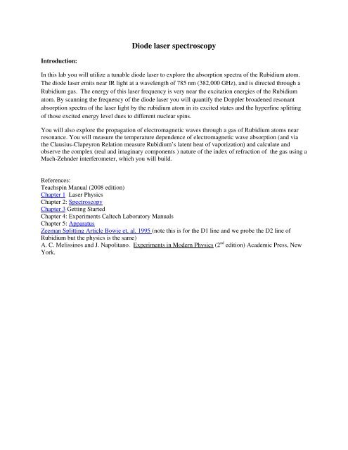
Diode laser spectroscopy

Diode laser spectroscopy
Introduction:
In this lab you will utilize a tunable diode laser to explore the absorption spectra of the Rubidium atom.
The diode laser emits near IR light at a wavelength of 785 nm (382,000 GHz), and is directed through a
Rubidium gas. The energy of this laser frequency is very near the excitation energies of the Rubidium
atom. By scanning the frequency of the diode laser you will quantify the Doppler broadened resonant
absorption spectra of the laser light by the rubidium atom in its excited states and the hyperfine splitting
of those excited energy level dues to different nuclear spins.
You will also explore the propagation of electromagnetic waves through a gas of Rubidium atoms near
resonance. You will measure the temperature dependence of electromagnetic wave absorption (and via
the Clausius-Clapeyron Relation measure Rubidium’s latent heat of vaporization) and calculate and
observe the complex (real and imaginary components ) nature of the index of refraction of the gas using a
Mach-Zehnder interferometer, which you will build.
References:
Teachspin Manual (2008 edition)
Chapter 1 Laser Physics
Chapter 2: Spectroscopy
Chapter 3 Getting Started
Chapter 4: Experiments Caltech Laboratory Manuals
Chapter 5: Apparatus
Zeeman Splitting Article Bowie et. al. 1995 (note this is for the D1 line and we probe the D2 line of
Rubidium but the physics is the same)
A. C. Melissinos and J. Napolitano. Experiments in Modern Physics (2 nd edition) Academic Press, New
York.

Theoretical Background:
The majority of the theoretical background behind using Doppler broadened Saturated Absorption
Spectroscopy to study Rubidium atoms can be found in Chapter 2 of the Teach Spin Manual
(Spectroscopy ). This includes discussion of how absorption peaks (and crossover resonances) come to
be, as well as the quantum mechanical background of the transitions in Rubidium. Below is a summary
of some of the useful information presented with little explanation.
Rubidium transitions:
From (Caltech Manual chapter 4.1):
Rubidium has two stable isotopes: 85 Rb (72 percent abundance), with nuclear spin quantum number I =
5/2, and 87 Rb (28 percent abundance), with I = 3/2. The different energy levels are labeled by “term
states”, with the notation 2S+1 L’ J , where S is the spin quantum number, L’ is the spectroscopic notation for
the angular momentum quantum number (i. e. S, P,D, . . ., for orbital angular momentum quantum
number L = 0, 1, 2, . . .), and J = L+S is the total angular momentum quantum number. For the ground
state of rubidium S = 1/2 (since only a single electron contributes), and L = 0, giving J = 1/2 and the
ground state 2S 1/2 . For the first excited state we have S = 1/2, and L = 1, giving J = 1/2 or J = 3/2, so there
are two excited states 2P 1/2 and 2P 3/2 . Spin-orbit coupling lifts splits the otherwise degenerate P 1/2 and P 3/2
levels. (See any good quantum mechanics or atomic physics text for a discussion of spin-orbit coupling.)
The dominant term in the interaction between the nuclear spin and the electron gives rise to the magnetic
hyperfine splitting (this is described in many quantum mechanics textbooks):
∆E =(C/2) [F(F +1) − I(I +1) − J(J +1)]
where F = I + J is the total angular momentum quantum number including nuclear spin, and C is the
“hyperfine structure constant.”
Figure 1: (Left) Level diagrams for the D2 lines of the two stable rubidium isotopes.
(Right) Typical absorption spectrum for a rubidium vapor cell, with the different lines shown. (From Teach Spin Manual
Chapter 2)

Figure 8: Rubidium energy level diagrams showing hyperfine splittings of the ground and excited states. Selection rules
for transitions are ∆F=0,+/-1.
Experimental apparatus:

Experimental setup shown above is enclosed within the Plexiglas box. Take some time to identify the
different parts (but don’t bump any of the optics). They should be aligned fairly well at this point, but you
may have to do some alignment as part of your lab work.
Our specific setup is shown on the following page.
In addition to the setup above, there is also:
1) The Laser control box (which controls laser temperature, current, and scanning frequencies)
2) CCD camera and TV
3) Digital Oscilloscope
4) Keithley multimeter
5) Notes on the laser: The laser should be aligned within the cavity. Do not remove its enclosure
box. If you have difficulty observing the laser, or any of the features, it is mostly likely because
of alignment of the optics, or settings on the electronics. You should be able to identify which and
how to remedy the situation.

90/10 bs
90/10 bs
mirror
mirror
50/50 bs
mirror
photodiodes
interferometer
50/50 bs
mirror
mirror

Safety:
• Before beginning this experiment Penn State Requires that all students operating a class IIIB laser
take the online laser safety training found by following the instructions here:
http://www.ehs.psu.edu/radprot/training_and_quiz.cfm
After your training is complete include a copy of your training certificate in the back of the Diode
laser spectroscopy 3-ring binder and add your name to the list of those who are specifically
trained for this experiment on the Laser Training Sheet at the back of the binder.
• Optical setup is enclosed within a Plexiglas case to prevent stray laser light from exiting the
experimental area.
• Note, the laser is infrared and you can’t see it directly, so there is no blink reflex if the laser hits
your eye, so you must wear safety goggles whenever the laser is on and the Plexiglas lid is off.
• Never put your head at eye level with the laser ON. Always look at the setup from above.
• When turning on the control box always make sure the LASER ON switch is turned off (down).
• Also, never touch the mirrors/beam splitters/optics devices, the surfaces will scratch when
cleaned and this can cause the laser to reflect improperly.
The experiment:
*Note below is an abbreviated description of how to measure the Rubidium spectrum. If the setup
is reasonably aligned this description will be sufficient. Otherwise refer to the Teachspin Manual
Chapter 3 and Chapter 4.1 (Caltech Experiment Manual).
Finding the laser beam: Place a business card in a holder between beam splitter 1 and beam splitter 2.
Also place a business card between photodiode detector 3 and the interferometer beam splitter. You will
not need this part of the optics path at this point. Turn on the control box and set the temperature to 50C,
wait until the temperature is stabilized, and then turn on the laser with the current dial at zero. Using the
IR viewing card, place the card directly in front of the laser output and slowly turn on the current until
you can see the orange spot on the card. (You may remove the neutral density filter directly in front of the
laser). This is how you will locate the laser beam, as you can’t see it with your eye. Now turn the laser off
again (no need to turn the current back down).
1) Varying the laser current:
a. Find the lasing current. To do this, focus the TV camera on the card. Dim the room
lights and turn the laser current to zero. Now increase the current while watching the
TV monitor. You will see a light spot that becomes slightly brighter as you increase
the current. Your diode laser is below threshold, it is not lasing, but only acting as an
LED. As you continue to increase the current you will observe a sudden brightening
of the beam spot and the appearance of a speckle pattern characteristic of lasing.
Adjust the current so that the laser is just above threshold. You can measure the laser
current with a voltmeter. A diode current of 50 mA will give 5.0 Volt output on the
LASER CURRENT in the MONITORS section. You can compare your measured
value with the threshold current recorded on your data sheet. A lower threshold
current represents better optical alignment. If the threshold current is significantly

different from that on the data sheet (1 st page of manual), the laser cavity will need to
be re-aligned.
2) Observing Rubidium Fluorescence:
a. Move the business card from between the beam splitters to be between beam splitter 2
and the first mirror. Use the orange card to assure the beam is hitting the business card.
For now we will focus on this simple part of the experimental setup:
b. Check that the 2 (why are there 2) laser beams enter the Rubidium gas and comes out the
other side (The neutral density filter can still be out at this point). Point the camera so it
looks into the Rb cell from the Side Hole in the cell heater. If you place the camera
up on the base of the cell holder you can position the camera so that it abuts the glass
holder surrounding the Rb cell.
c. Observe the RAMP OUTPUT of the RAMP GENERATOR module on an oscilloscope using
the RAMP GENERATOR SYNC. OUTPUT as a trigger. Observe the output on the ‘scope as
you adjust the RAMP GENERATOR settings.
d. Use the RAMP GENERATOR and PIEZO CONTROLLER to Set the Frequency Sweep
i. Turn the ramp amplitude down and connect the RAMP OUTPUT from the
oscilloscope to the modulation input connection on the PIEZO CONTROLLER
MODULE.
ii. Connect the MONITOR OUTPUT of the PIEZO to Channel 1 of the oscilloscope.
Turn the piezo OUTPUT OFFSET knob to zero. (The OUTPUT OFFSET
changes the DC level of the monitor output. It does not change the voltage
applied to the piezo stack.
iii. Set the ramp generator frequency to about 10 Hz. Turn the piezo
ATTENUATOR knob to one (1). Set the ramp generator AMPLITUDE knob
to ten (10) and use the DC OFFSET knob of piezo controller to produce a
large-amplitude triangle wave that is not clipped at the top or bottom. The
piezo MONITOR OUTPUT should have a signal that runs from about 3 volts
to about 8 volts. (You should know what the piezo is doing before you move
on)
e. Find the minimum laser current that creates rubidium fluorescence, and compare it to
the value on the front page of the manual.
3) Rubidium Doppler Broadened absorption peaks
a. Check that each of the 2 beams are going to detector 1 and detector 2, respectively. At
this point you should return the neutral density filter to its location. Using detector 2,
view the output of the Photodiode detector on the ‘scope on channel 2. The signal from
the Photodiode Detector is negative and saturates at about -11.0 volts. If the signal is
saturated turn down the gain on the back of the photodiode until you see a signal. For
the best performance you want the PD Gain to be as high as possible without
saturating the PD, a signal level of 2 to 6 volts is reasonable. Block the beam with

your hand to convince yourself that the PD is detecting the transmitted laser light.
You may have to wiggle the photodiode to maximize the signal going to the detector.
You should see a ‘scope signal that looks something like this:
b. The absorption dips in your trace are interrupted by various “mode hops” – why do
these occur? Observe how the signal changes when you vary the laser current and the
piezo drive parameters. With proper adjustment you should be able to set a scan that
covers the first three lines in the absorption spectrum. (You should understand the
physics of why these absorption peaks exist, and why they have some width)
c. Using Simultaneous Current and Piezo Modulation to produce a larger scan range
without mode hops.
i. Set the laser CURRENT ATTENUATOR knob to zero. Attach the BNC splitter
“F” connector to the RAMP OUTPUT on the RAMP GENERATOR. Plug one BNC
from the RAMP OUTPUT to the MODULATION INPUT of the PIEZO CONTROLLER,
and the second BNC from RAMP OUTPUT to the CURRENT MODULATION INPUT.
ii. Turn the ramp generator amplitude up to maximum, and watch what happens
when you turn up the current attenuator knob. With some tweaking you
should be able to produce a full trace over the Rb spectrum.
a. Record the spectra and measure frequency shifts between absorption peaks and peak
widths.
i. To do this you will need to calibrate the observed spectra with the interference
fringes measured with the Michelson Interferometer (detector 3). You will have
to remove the beam block in front of detector 3, and make sure the detector is
positioned to see the laser beam, and adjust the gain on the photodiode to observe
the fringe pattern. You should get something like the figure below on the ’scope
if you are doing everything right:

i. You may need to adjust and align the optics of the Michelson Interferometer.
To setup and align the Michelson Interferometer follow the steps in the manual
(pages 3.26-3.30 of Chapter 3).
ii. Once you have the Interferometer aligned, return the laser frequency to
scanning mode- you should observe oscillations on the photodiode output
shown on the oscilloscope. When a beam travels a distance L it picks up a
phase 2πL/λ, so the electric field becomes ϕ
iii.
When the beam is split in the interferometer, the two parts are sent down the two
arms, making the combined electric field
E = E arm1 + E arm2 = E 0 e iωt( e i4πL 1 /λ + e i4πL2/λ )
where L1 and L2 are the two arm lengths. The additional factor of two comes
from the fact that the beam goes down the arm and back again. Squaring this to
get the intensity we have
I ~(e i4πL1/λ + e i4πL2/λ ) 2 ~ 1 + cos(4π∆L/λ)
where ∆L = L1 − L2. If the laser frequency is constant, then the fringe pattern
goes through one cycle every time the arm length changes by λ/2. If ∆L is fixed,
E0eiωteiϕ
what is the fringe period in MHz?
Use the two oscilloscope traces to plot the interferometer fringes and the
saturated absorption spectra at the same time, as you scan the laser frequency.
You will use the Michelson Interferometer in the next step as well.
=
E =
4) Observing the Saturated Absorption Spectra and Measuring the hyperfine splitting of
Rubidium:
a. From the non-saturated absorption spectra you should have noticed there are four excited
energy states of Rubidium which you can probe with the laser. Each of these excited
energy states has a hyperfine splitting due to nuclear spin states. The frequencies of these
hyperfine states are observed as spikes in the absorption peaks (why are they spikes?).
Added features called crossover resonances are also observed. These are
additional narrow absorption dips arising because several upper or lower energy
levels are close enough in energy that their Doppler-broadened profiles overlap
creating an extra absorption spike between each of the expected peaks. Before you
measure the hyperfine splitting of each of the four excited states, you should make 4
graphs (one for each absorption peak) showing the expected frequency peaks, including

the crossover peaks for each of the four possible transition scenarios given that the
selection rule is ∆F=0,+/-1. Crossover peaks are found half-way between each of the
expected peaks (ν 1 +ν 2 )/2 for two absorption peaks of frequency ν 1 and ν 2 . Refer to the
manual section on Spectroscopy for an explanation of the quantum mechanics involved,
and for hints about crossover resonances.
b. Re-connect the current modulation for this part of the experiment. Remove beam block
between the second beam splitter and the first mirror. Chances are you will have to align
the optic such that there are three beams passing through the rubidium chamber, two
weak probe beams which are split of the 90/10 beamsplitter, and a third which is directed
back through the rubidium chamber which acts as a pump beam. You should know what
the roles are of these two beams. The resulting SAS spectra will be observed in the
photodiode detector #1. You may observe this directly on the ‘scope.
c. Expand the scale so that you can observe the two large absorption features. If your
beams are close to being aligned, you will start to see some sharp spikes within the
broad absorptions – you should know why you see spikes, ie, why has the absorption
decreased? If they are not well aligned, you will have to re-align the beams using the
instructions in the manual. You may now try to maximize the size of these spikes by
gently wiggling the adjustment screws on the mirrors and the 50/50 BS.
d. Compare the spectra observed in Photodiode 1 to that in Photodiode 2. It is useful to use
the detector electronics section of your electronics box to isolate that difference
between these two signals. Put the signal from Detector 1 into the minus input and
that from Detector 2 into the plus input of the detector section of the electronics box.
Attach the monitor output to the ‘scope. Set the plus balance control to zero and the
minus balance control to one and observe the signal from Detector 1 on the ‘scope.
Adjust the gain on Detector 1 so that you have a large signal (several volts) but not so
large as to saturate the detector (maximum signal less than 10 volts). Now, set the
plus balance to one and the minus balance to zero and observe the signal form
Detector 2. It will be inverted, with negative voltage values. Again adjust the gain of
Detector 2 for a signal level that is comparable to that seen by Detector 1. Because
the beam going to Detector 2 is not attenuated by the 50/50 beam splitter, the gain
needed on Detector 2 will be less than that of Detector 1.
e. Now set both balance knobs to one and then reduce the balance on the larger signal so
that the Doppler broadened background is removed. This subtraction is never perfect,
so there will always be some residual broad absorption signal remaining. You may
now raise the gain setting on the difference signal and bring the SAS spikes up to the
volt level.
f. Measure the hyperfine splitting for each of the 4 Doppler broadened absorption lines. (To
get a good picture of the spectra for each of the 4 lines, it is useful to tune the piezo
voltage slightly until you see one line clearly (on the left of the o-scope), and then
increase the resolution on the scope, and then optimize the electronic subtraction.
Quantify the frequency shifts using the Michelson Interferometer.
5) Measuring the Zeeman splitting of the magnetic moments of Rubidium:
The 10 Ohm Helmholtz coils surrounding the Rubidium chamber can be used to create a
magnetic field up to 10 mT when 3A of current are supplied to them. Using the voltage source
available apply a minimum amount of current to the Helmholtz coils in order to observe magnetic
field induced splitting of the hyperfine split lines. Your goal should be to try to discern the
splitting due to the different magnetic moments available for the excited Rubidium atoms. An

excellent reference is the published paper included in the manual on the Zeeman Effect in
Rubidium. By measuring the change in energy of a magnetically induced absorption peak as a
function of magnetic field, you might be able to experimentally measure g the gyromagnetic ratio
which relates energy to magnetic field via:
∆E= g F µ b B M F ,
where
g F =g J (F(F+1)+J(J+1)-I(I+1))/[2F(F+1)]
and M F is the magnetic quantum number. Allowed transitions are determined by whether the
photons are left (∆M F =+1) or right (∆M F =-1) cicularly polarized.
6) Interferometric Measurement of Resonant Absorption and Refractive Index in Rubidium
a. NOTE: often other groups are using the same apparatus. Make sure to discuss with all
student groups before changing the optical setup.
b. Before you do this experiment you should complete problems #1 and #2 in the Caltech
experiment manual with the same title (found in the Teach-Spin manual section 4.2).
c. Measure temperature dependence of the fractional absorption (use the 85a line) of
Rubidium to calculate the latent heat of vaporization of Rubidium for one peak in the
absorption spectra. (See attached pages) You will have to disconnect the current sweep to
do this measurement. Block the pump beam before it enters beamsplitter #2, and use the
probe beam entering detector #2. You should also chose one temperature and vary the
laser current to measure the current dependence of the fractional absorption.
d. To measure the frequency dependence of the index of refraction you will need to rearrange
and align the optics to create the Mach-Zehnder interferometer. This is most
easily done by replacing beamsplitter #1 in the diagram with a 50/50 beam splitter,
removing beamsplitter #2, and switching the locations of beamsplitter #3 and mirror #2
(not the one in the Michelson interferometer).
e. To align the interferometer, turn off the frequency and current scanning on the electronics
box, and remove the rubidium chamber (after assuring that the laser goes through the
rubidium chamber’s window). Follow instructions in the manual to align the
interferometer. After you have the two beams parallel and overlapping, move detector #3
to intercept the beam. Use the output from detector three to optimize the amplitude of the
interference between the two beams (follow Caltech instructions about wiggling the
mirrors and adjusting until the amplitude of the wiggled signal is >0.8 of the DC voltage).
f. After the interferometer is aligned, re-insert the Rubidium chamber, and add a cartridge
filter in between the chamber and the mirror. Increase the current such that the Rubidium
fluoresces, and re-assess the interference amplitude (it may require further tweaking).
g. Turn on the frequency scanning, and place a business card in the path of the laser beam
that does not traverse the Rubidium chamber. Verify that you have a nice Doppler
broadened spectra with no mode hops, and center the 85b line in the middle of the
oscilloscope.
h. Follow the Caltech instructions to capture the spectra at different phases at low and high
temperature. Attempt to match those spectra to those you calculated, and relate the
spectra you observed with the temperature dependent absorption.
i. Return optics to the original configuration in the diagram above.