Nanosurf easyScan 2 AFM Operating Instructions
Nanosurf easyScan 2 AFM Operating Instructions
Nanosurf easyScan 2 AFM Operating Instructions

Create successful ePaper yourself
Turn your PDF publications into a flip-book with our unique Google optimized e-Paper software.
<strong>Nanosurf</strong><br />
<strong>easyScan</strong> 2 <strong>AFM</strong><br />
<strong>Operating</strong> <strong>Instructions</strong><br />
for<br />
SPM Control Software<br />
Version 3.0
“NANOSURF” AND THE NANOSURF LOGO ARE TRADEMARKS OF NANOSURF AG,<br />
REGISTERED AND/OR OTHERWISE PROTECTED IN VARIOUS COUNTRIES.<br />
COPYRIGHT © JULY 2011, NANOSURF AG, SWITZERLAND.<br />
OPERATING INSTRUCTIONS V3.0R1, BT02089-13.
Table of contents
Table of contents<br />
CHAPTER 1: The <strong>easyScan</strong> 2 <strong>AFM</strong> 11<br />
1.1: Introduction.............................................................................................. 12<br />
1.2: Components of the system ...................................................................... 13<br />
1.2.1: Contents of the Tool Set .................................................................................14<br />
1.3: Connectors, indicators and controls ....................................................... 15<br />
1.3.1: The <strong>easyScan</strong> 2 <strong>AFM</strong> Scan Head ..................................................................15<br />
1.3.2: The <strong>easyScan</strong> 2 Controller..............................................................................16<br />
CHAPTER 2: Installing the <strong>easyScan</strong> 2 <strong>AFM</strong> 19<br />
2.1: Installing the hardware............................................................................ 20<br />
2.1.1: Installing the <strong>easyScan</strong> 2 controller ...........................................................20<br />
2.1.2: Installing the <strong>AFM</strong> Video Camera................................................................21<br />
2.1.3: Installing the Signal Module S......................................................................21<br />
2.1.4: Installing the Signal Module A and its Connector Box........................22<br />
2.1.5: Installing the <strong>easyScan</strong> 2 <strong>AFM</strong> Scan Head ...............................................22<br />
2.2: Installing the SPM Control Software....................................................... 23<br />
2.2.1: Preparations before installing ......................................................................23<br />
2.2.2: Initiating the installation procedure ..........................................................24<br />
2.2.3: Hardware recognition .....................................................................................25<br />
2.2.4: Manual installation of the USB Video Adapter driver ..........................25<br />
CHAPTER 3: Preparing for measurement 27<br />
3.1: Introduction.............................................................................................. 28<br />
3.2: Initializing the <strong>easyScan</strong> 2 Controller..................................................... 28<br />
3.3: Installing the cantilever ........................................................................... 29<br />
3.3.1: Selecting a cantilever ......................................................................................30<br />
3.3.2: Inserting the cantilever in the Scan Head................................................31<br />
3.4: Installing the sample................................................................................ 34<br />
3.4.1: Preparing the sample ......................................................................................34<br />
3.4.2: <strong>Nanosurf</strong> samples .............................................................................................34<br />
3.4.3: Stand-alone measurements..........................................................................37<br />
3.4.4: The Sample Stage .............................................................................................38<br />
3.4.5: Mounting a sample ..........................................................................................38<br />
CHAPTER 4: A first measurement 41<br />
4.1: Introduction.............................................................................................. 42<br />
4.2: Running the microscope simulation....................................................... 42<br />
4.3: Preparing the instrument ........................................................................ 43<br />
4.3.1: Entering and changing parameter values ...............................................43<br />
4
4.4: Approaching the sample ......................................................................... 44<br />
4.4.1: Manual coarse approach................................................................................45<br />
4.4.2: Manual approach using the motorized approach stage....................46<br />
4.4.3: Automatic final approach ..............................................................................47<br />
4.5: Starting a measurement .......................................................................... 49<br />
4.6: Selecting a measurement area................................................................ 50<br />
4.7: Storing the measurement........................................................................ 52<br />
4.8: Creating a basic report............................................................................. 53<br />
4.9: Further options......................................................................................... 53<br />
CHAPTER 5: Improving measurement quality 55<br />
5.1: Removing interfering signals.................................................................. 56<br />
5.1.1: Mechanical vibrations .....................................................................................56<br />
5.1.2: Electrical interference......................................................................................56<br />
5.1.3: Infrared or other light sources......................................................................57<br />
5.2: Adjusting the measurement plane ......................................................... 57<br />
5.3: Judging tip quality ................................................................................... 60<br />
CHAPTER 6: <strong>Operating</strong> modes 63<br />
6.1: Introduction.............................................................................................. 64<br />
6.2: Static Force mode ..................................................................................... 64<br />
6.3: Dynamic Force mode................................................................................ 65<br />
6.4: Phase Contrast mode ............................................................................... 65<br />
6.5: Force Modulation mode........................................................................... 67<br />
6.6: Spreading Resistance mode .................................................................... 68<br />
6.7: Kelvin Probe Force Microscopy ............................................................... 69<br />
6.7.1: Introduction........................................................................................................69<br />
6.7.2: <strong>Operating</strong> principle..........................................................................................69<br />
6.7.3: System requirements.......................................................................................70<br />
6.7.4: Procedures...........................................................................................................72<br />
CHAPTER 7: Finishing measurements 81<br />
7.1: Finishing scanning ................................................................................... 82<br />
7.2: Turning off the instrument ...................................................................... 82<br />
7.3: Storing the instrument ............................................................................ 83<br />
CHAPTER 8: Maintenance 85<br />
8.1: Introduction.............................................................................................. 86<br />
8.2: The <strong>easyScan</strong> 2 <strong>AFM</strong> Scan Head .............................................................. 86<br />
8.3: The <strong>easyScan</strong> 2 controller........................................................................ 86<br />
CHAPTER 9: Problems and solutions 87<br />
9.1: Introduction.............................................................................................. 88<br />
5
9.2: Software and driver problems ................................................................ 88<br />
9.2.1: No connection to microscope......................................................................88<br />
9.2.2: USB Port error.....................................................................................................88<br />
9.2.3: Driver problems.................................................................................................89<br />
9.3: <strong>AFM</strong> measurement problems .................................................................. 91<br />
9.3.1: Probe Status light blinks red.........................................................................91<br />
9.3.2: Automatic final approach fails .....................................................................92<br />
9.3.3: Image quality suddenly deteriorates.........................................................92<br />
9.4: <strong>Nanosurf</strong> support ..................................................................................... 93<br />
9.4.1: Self help................................................................................................................93<br />
9.4.2: Assistance ............................................................................................................94<br />
CHAPTER 10: <strong>AFM</strong> theory 95<br />
10.1: Scanning probe microscopy .................................................................... 96<br />
10.2: The <strong>easyScan</strong> 2 <strong>AFM</strong> ................................................................................. 97<br />
CHAPTER 11: Technical data 99<br />
11.1: Introduction............................................................................................. 100<br />
11.2: The <strong>easyScan</strong> 2 <strong>AFM</strong> Scan Heads............................................................ 100<br />
11.2.1: Specifications and features ..........................................................................100<br />
11.2.2: Dimensions ........................................................................................................101<br />
11.3: The <strong>easyScan</strong> 2 Controller ...................................................................... 102<br />
11.3.1: Hardware features and specifications ......................................................102<br />
11.3.2: Software features and computer requirements ...................................102<br />
11.4: Hardware modules and options............................................................. 104<br />
11.4.1: <strong>AFM</strong> modules ....................................................................................................104<br />
11.4.2: The Signal Modules.........................................................................................105<br />
11.4.3: The <strong>AFM</strong> Video Module .................................................................................108<br />
11.4.4: The Micrometer Translation Stage.............................................................108<br />
CHAPTER 12: The SPM Control Software user interface 109<br />
12.1: General concept and layout.................................................................... 110<br />
12.2: The workspace ......................................................................................... 111<br />
12.3: <strong>Operating</strong> windows................................................................................. 112<br />
12.4: Document space ...................................................................................... 113<br />
12.5: Panels ....................................................................................................... 114<br />
12.6: Ribbon ...................................................................................................... 116<br />
12.7: Status bar ................................................................................................. 117<br />
12.8: View tab.................................................................................................... 118<br />
12.8.1: Workspace group.............................................................................................118<br />
12.8.2: Panels group......................................................................................................118<br />
12.8.3: Window group ..................................................................................................119<br />
6
CHAPTER 13: Imaging 121<br />
13.1: Introduction............................................................................................. 122<br />
13.2: Imaging panel.......................................................................................... 123<br />
13.3: The Imaging toolbar................................................................................ 127<br />
13.4: Acquisition tab ........................................................................................ 128<br />
13.4.1: Preparation group ...........................................................................................129<br />
13.4.2: Approach group ...............................................................................................130<br />
13.4.3: Imaging group ..................................................................................................131<br />
13.4.4: Scripting group.................................................................................................132<br />
13.5: Stage panel .............................................................................................. 133<br />
13.5.1: Move Stage To dialog .....................................................................................134<br />
13.6: Video panel .............................................................................................. 135<br />
13.6.1: Analog video camera display ......................................................................136<br />
13.6.2: Digital Video Camera display.......................................................................137<br />
13.6.3: Illumination section ........................................................................................140<br />
13.6.4: Digital Video Properties dialog ...................................................................140<br />
13.7: Online panel............................................................................................. 142<br />
13.7.1: Scan Position section......................................................................................142<br />
13.7.2: Master Image section .....................................................................................143<br />
13.7.3: Illumination section ........................................................................................144<br />
CHAPTER 14: Spectroscopy 145<br />
14.1: Introduction............................................................................................. 146<br />
14.2: Spectroscopy panel................................................................................. 148<br />
14.3: Spectroscopy toolbar.............................................................................. 149<br />
14.4: Acquisition tab ........................................................................................ 150<br />
14.4.1: Spectroscopy group........................................................................................150<br />
CHAPTER 15: Lithography 151<br />
15.1: Introduction............................................................................................. 152<br />
15.2: Performing lithography.......................................................................... 153<br />
15.3: Lithography panel................................................................................... 154<br />
15.3.1: Layer Editor dialog...........................................................................................157<br />
15.3.2: Object Editor dialog........................................................................................159<br />
15.4: Acquisition tab ........................................................................................ 160<br />
15.4.1: Lithography group ..........................................................................................160<br />
15.5: Lithography toolbar................................................................................ 161<br />
15.5.1: Vector Graphic Import dialog......................................................................163<br />
15.5.2: Pixel Graphic Import dialog .........................................................................165<br />
15.6: Lithography preview............................................................................... 168<br />
7
CHAPTER 16: Working with documents 169<br />
16.1: Introduction............................................................................................. 170<br />
16.2: Data Info panel ........................................................................................ 170<br />
16.2.1: Data Info toolbar ..............................................................................................171<br />
16.3: Charts ....................................................................................................... 171<br />
16.3.1: Working with multiple charts......................................................................173<br />
16.3.2: Chart Properties dialog..................................................................................174<br />
16.4: Gallery panel............................................................................................ 181<br />
16.4.1: History File mask ..............................................................................................182<br />
16.4.2: Image list.............................................................................................................182<br />
16.4.3: Gallery toolbar ..................................................................................................182<br />
16.4.4: Mask Editor dialog ...........................................................................................183<br />
16.4.5: File Rename dialog ..........................................................................................185<br />
16.5: Analysis tab.............................................................................................. 186<br />
16.5.1: Measure group..................................................................................................187<br />
16.5.2: Correction group..............................................................................................189<br />
16.5.3: Roughness group.............................................................................................191<br />
16.5.4: Filter group.........................................................................................................193<br />
16.5.5: Tools group ........................................................................................................195<br />
16.5.6: Report Group.....................................................................................................196<br />
16.5.7: Scripting group.................................................................................................198<br />
16.6: Tool panel................................................................................................. 198<br />
CHAPTER 17: Advanced settings 201<br />
17.1: About dialog ............................................................................................ 202<br />
17.2: File menu.................................................................................................. 203<br />
17.2.1: Options dialog ..................................................................................................206<br />
17.3: Settings tab.............................................................................................. 212<br />
17.3.1: Scan Head group..............................................................................................213<br />
17.3.2: Hardware group ...............................................................................................213<br />
17.4: Scan Head Selector dialog ...................................................................... 214<br />
17.5: Scan Head Calibration Editor dialog...................................................... 215<br />
17.5.1: Scan Axis .............................................................................................................215<br />
17.5.2: I/O Signals...........................................................................................................216<br />
17.6: Scan Axis Correction dialog.................................................................... 218<br />
17.7: Scan Head Diagnosis dialog ................................................................... 218<br />
17.7.1: Dialog for <strong>AFM</strong> scan heads ...........................................................................219<br />
17.7.2: Dialog for STM scan head .............................................................................219<br />
17.8: Controller Configuration dialog............................................................. 220<br />
8
17.9: SPM Parameters dialog........................................................................... 221<br />
17.9.1: Imaging ...............................................................................................................222<br />
17.9.2: Spectroscopy.....................................................................................................225<br />
17.9.3: Lithography........................................................................................................228<br />
17.9.4: <strong>Operating</strong> Mode...............................................................................................229<br />
17.9.5: Approach ............................................................................................................231<br />
17.9.6: Z-Controller........................................................................................................233<br />
17.9.7: Signal Access .....................................................................................................235<br />
17.10: User Signal Editor dialog........................................................................ 238<br />
17.11: Vibration Frequency Search dialog ....................................................... 239<br />
17.11.1: General concept ...............................................................................................239<br />
17.11.2: Automated vibration frequency search...................................................240<br />
17.11.3: Manual sweep controls..................................................................................241<br />
17.11.4: Auto Frequency Config dialog ....................................................................243<br />
17.12: Laser Alignment dialog .......................................................................... 244<br />
17.13: Cantilever Browser dialog ...................................................................... 245<br />
17.13.1: Cantilever Editor dialog .................................................................................247<br />
17.14: ATS Stage and TSC 3000 driver configuration ...................................... 248<br />
17.14.1: Stage Configuration dialog ..........................................................................250<br />
17.14.2: The COM Port Configuration dialog..........................................................252<br />
Quick reference 253<br />
9
About this Manual<br />
This manual is divided into two parts: The first part provides instructions on how to set up<br />
and use your <strong>Nanosurf</strong> <strong>easyScan</strong> 2 <strong>AFM</strong> system. The second part is a reference for the<br />
software that comes with the <strong>easyScan</strong> 2 <strong>AFM</strong> system. It applies to <strong>Nanosurf</strong> SPM Control<br />
Software version 3.0. If you are using newer software versions, download the latest manual<br />
from the <strong>Nanosurf</strong> support pages, or refer to the “What’s new in this version.pdf” file that is<br />
installed in the Manuals subdirectory of the directory where the SPM Control Software is<br />
installed.<br />
The first part of the manual starts with Chapter 1: Introduction (page 12), which provides an<br />
introduction to the <strong>easyScan</strong> 2 <strong>AFM</strong> system, and with Chapter 2: Installing the <strong>easyScan</strong> 2<br />
<strong>AFM</strong> (page 19), which should be read when installing your system. Chapter 3: Preparing for<br />
measurement (page 27) and Chapter 4: A first measurement (page 41) should be read by all<br />
users, because they contain useful instructions for everyday measurements. The other<br />
chapters provide more information for advanced or interested users.<br />
The second part of the manual can be used as a reference for the SPM Control Software that<br />
controls the <strong>AFM</strong>. It starts with Chapter 12: The SPM Control Software user interface (page<br />
109) and ends with Chapter 17: Advanced settings (page 201). This part describes the<br />
functions of all buttons, inputs, dialogs, and control panels of the SPM Control Software.<br />
The final chapter of this manual, Quick reference (page 254), contains an index to the<br />
software reference part of the manual for quick retrieval of the relevant information<br />
locations.<br />
For more information on the scripting interface of the software packages, refer to the online<br />
help file <strong>easyScan</strong> 2 Script Programmers Manual that is installed together with the SPM<br />
Control Software.<br />
For more information on the optional <strong>Nanosurf</strong> Report software, refer to the on-line help<br />
included with the <strong>Nanosurf</strong> Report software.
CHAPTER 1:<br />
The <strong>easyScan</strong> 2 <strong>AFM</strong><br />
0<br />
0
CHAPTER 1: THE EASYSCAN 2 <strong>AFM</strong><br />
1.1: Introduction<br />
The <strong>Nanosurf</strong> <strong>easyScan</strong> 2 <strong>AFM</strong> system is an atomic force microscope that can measure the<br />
topography and several other properties of a sample with nanometer resolution. These<br />
measurements are performed, displayed, and evaluated using the SPM Control Software.<br />
The <strong>easyScan</strong> 2 <strong>AFM</strong> system is a modular scanning probe system that can be upgraded to<br />
obtain more measurement capabilities. The main parts of the basic system are the<br />
<strong>easyScan</strong> 2 <strong>AFM</strong> Scan Head, the <strong>AFM</strong> Sample stage, the <strong>easyScan</strong> 2 Controller with <strong>AFM</strong><br />
Basic module, and the SPM Control Software.<br />
The content of the system and the function of its major components are described in this<br />
chapter. Detailed technical specifications and system features can be found in Chapter 11:<br />
Technical data (page 99).<br />
Several other <strong>Nanosurf</strong> products can be used in conjunction with the <strong>easyScan</strong> 2 <strong>AFM</strong>:<br />
• <strong>AFM</strong> Dynamic Module: adds dynamic mode measurement capabilities for measuring<br />
delicate samples.<br />
• <strong>AFM</strong> Mode Extension Module: adds phase contrast, force modulation and current<br />
measurement capabilities.<br />
• <strong>AFM</strong> Video Module: allows observation of the approach on the computer screen. This is<br />
useful when observation using the lenses is impractical.<br />
• Signal Modules: allow monitoring signals (Module S) and creating custom operating<br />
modes (Module A). Refer to Section 11.4.2: The Signal Modules (page 105) for more details.<br />
• <strong>Nanosurf</strong> Micrometer Translation Stage: allows locating of a position on a sample with<br />
micrometer accuracy. Should be used together with the <strong>Nanosurf</strong> <strong>easyScan</strong> 2 Sample<br />
Stage.<br />
• <strong>Nanosurf</strong> Report: software for simple automatic evaluation and report generation of<br />
SPM measurements.<br />
• <strong>Nanosurf</strong> Analysis: software for detailed analysis of SPM measurements.<br />
• Scripting Interface: software for automating measurements. Refer to Section 13.4.4:<br />
Scripting group (page 132) and the Programmer’s Manual for more details.<br />
• Lithography Option: software for professional lithography applications. Refer to Chapter<br />
15: Lithography (page 151) for more information.<br />
• The <strong>Nanosurf</strong> isoStage: a highly compact active vibration isolation table, equipped with<br />
a special <strong>easyScan</strong> 2 <strong>AFM</strong> Sample Stage (The isoStage Adapter Plate), and dedicated for<br />
use with <strong>Nanosurf</strong> <strong>AFM</strong> scan heads.<br />
• The Halcyonics_i4 Active Vibration Isolation Table: a larger and heavier active vibration<br />
isolation solution, which features load adjustment.<br />
12
COMPONENTS OF THE SYSTEM<br />
1.2: Components of the system<br />
This section describes the parts that may be delivered with an <strong>easyScan</strong> 2 <strong>AFM</strong> system. The<br />
contents of delivery can vary from system to system, depending on which parts were<br />
ordered. To find out which parts are included in your system, refer to the delivery note<br />
shipped with your system. Some of the modules listed in the delivery note are built into the<br />
controller. Their presence is indicated by the status lights on the top surface of the<br />
controller when it is turned on (see Section 1.3.2: The <strong>easyScan</strong> 2 Controller (page 16)).<br />
1<br />
2<br />
3<br />
4 5 6<br />
7<br />
8 9<br />
17<br />
18<br />
19<br />
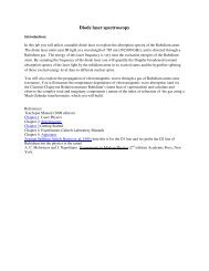
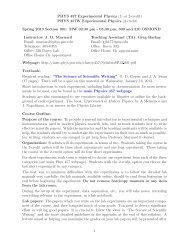
Figure 1-1: Components. The <strong>easyScan</strong> 2 <strong>AFM</strong> system<br />
1. <strong>easyScan</strong> 2 Controller with a built-in <strong>AFM</strong> Basic Module, and optionally with built-in<br />
<strong>AFM</strong> Dynamic Module, <strong>AFM</strong> Mode Extension Module, Video Module electronics and<br />
Signal Module A or S electronics.<br />
2. <strong>easyScan</strong> 2 <strong>AFM</strong> Scan Head(s) with <strong>AFM</strong> Video Camera (comes with <strong>AFM</strong> Video<br />
Module).<br />
3. Scan Head Case.<br />
4. USB cable.<br />
5. Mains cable.<br />
6. Scan Head cable, connects the Scan Head to the <strong>easyScan</strong> 2 controller.<br />
7. Video Camera cable (see item 2; comes with <strong>AFM</strong> Video Module).<br />
13
CHAPTER 1: THE EASYSCAN 2 <strong>AFM</strong><br />
8. <strong>AFM</strong> Sample stage (option).<br />
9. <strong>AFM</strong> Tool set (option). The items contained in the <strong>AFM</strong> Tool set are described in the<br />
next section.<br />
10. The <strong>easyScan</strong> 2 Installation CD (not shown): Contains software, calibration files, and<br />
PDF files of all manuals.<br />
11. A calibration certificate for each <strong>easyScan</strong> 2 <strong>AFM</strong> Scan Head (not shown).<br />
12. This <strong>easyScan</strong> 2 <strong>AFM</strong> <strong>Operating</strong> <strong>Instructions</strong> manual (not shown).<br />
13. <strong>AFM</strong> Extended Sample Kit (option; not shown), which comes with a set of 10 samples<br />
and description of experiments.<br />
14. Micrometer Translation Stage (option; not shown).<br />
15. User's Guide; Translation Stage, Model 9064 (not shown; comes with Micrometer<br />
Translation Stage).<br />
16. Positioning Tool Set (not shown; comes with the Micrometer Translation Stage).<br />
17. Break-out cable (comes with Signal Module S).<br />
18. Connector box (comes with Signal Module A).<br />
19. Two Signal Module cables (come with Signal Module A).<br />
20. Scripting Interface certificate of purchase with Activation key printed on it (not shown;<br />
comes with Scripting Interface).<br />
21. Lithography Option certificate of purchase with Activation key printed on it (not<br />
shown; comes with the Lithography Option).<br />
22. Instrument Case (not shown).<br />
The package may also contain <strong>easyScan</strong> 2 STM head(s) and modules for the STM, which are<br />
described in the <strong>easyScan</strong> 2 STM <strong>Operating</strong> <strong>Instructions</strong>.<br />
Please keep the original packaging material (at least until the end of the warranty period),<br />
so that it may be used for transport at a later date, if necessary. For information on how to<br />
store, transport, or send in the instrument for repairs, see Section 7.3: Storing the instrument<br />
(page 83).<br />
1.2.1: Contents of the Tool Set<br />
The content of the Tool set depends on the modules and options included in your order. It<br />
may contain any of the following items:<br />
1. Ground cable.<br />
2. Protection feet.<br />
3. Cantilever tweezers: (103A CA).<br />
4. Screwdriver, 2.3 mm.<br />
14
CONNECTORS, INDICATORS AND CONTROLS<br />
1 2 3<br />
4<br />
5<br />
6<br />
7<br />
8<br />
9 10<br />
11<br />
12<br />
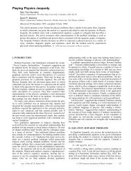
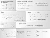
Figure 1-2: Contents of the Tool set<br />
5. Cantilever insertion tool (usually mounted in the DropStop).<br />
6. DropStop.<br />
7. Sample holder (comes as an option with the <strong>AFM</strong> Sample Stage).<br />
8. Samples (option). Possible combinations are:<br />
a. <strong>AFM</strong> Large Scan Sample Kit (Grid: 10 μm / 100 nm, CD ROM piece).<br />
b. <strong>AFM</strong> High Resolution Sample Kit (Grid: 660 nm, Graphite (HOPG) sample on<br />
sample support).<br />
c. Two calibration samples (Calibration grid: 10 μm / 100 nm, Calibration grid:<br />
660 nm).<br />
9. <strong>AFM</strong> Calibration Samples Kit (option) with three calibration samples (Calibration grid:<br />
10 μm / 100 nm, Calibration grid: 660 nm, Flatness sample).<br />
10. Set of 10 Static mode cantilevers (option).<br />
11. Set of 10 Dynamic mode cantilevers (option).<br />
12. USB dongle for <strong>Nanosurf</strong> Report or <strong>Nanosurf</strong> Analysis software (option).<br />
1.3: Connectors, indicators and controls<br />
Use this section to find the location of the parts of the <strong>easyScan</strong> 2 <strong>AFM</strong> that are referred to<br />
in this manual.<br />
1.3.1: The <strong>easyScan</strong> 2 <strong>AFM</strong> Scan Head<br />
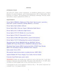
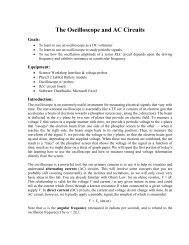
The location of the scan head parts listed below is shown in Figure 1-3: Parts of the Scan<br />
Head.<br />
15
CHAPTER 1: THE EASYSCAN 2 <strong>AFM</strong><br />
Levelling<br />
screws<br />
Scan head<br />
serial number<br />
Hole for cantilever<br />
insertion tool<br />
Camera<br />
connector<br />
Ground<br />
connector<br />
Scan head cable<br />
connector<br />
Cantilever on<br />
alignment chip<br />
Figure 1-3: Parts of the Scan Head. Scan Head with video Camera.<br />
Leveling screws<br />
For coarse approach of the sample (Section 4.4.1: Manual coarse approach (page 45)), and<br />
for aligning the plane of the scanner with the plane of the sample (Section 5.2: Adjusting the<br />
measurement plane (page 57)).<br />
Scan Head cable connector<br />
For connecting the Scan Head cable that also connects to the <strong>easyScan</strong> 2 Controller.<br />
Ground connector<br />
For connecting a cable that puts the sample or the Sample Holder at the same ground<br />
potential as the scan head.<br />
Alignment chip and hole for cantilever insertion tool<br />
Used for mounting the cantilever on the scan head (Section 3.3: Installing the cantilever<br />
(page 29)).<br />
Scan Head serial number<br />
Shows what serial number and version of the scan head you have.<br />
1.3.2: The <strong>easyScan</strong> 2 Controller<br />
Status lights<br />
All status lights on top of the controller will light up for one second when the power is<br />
turned on.<br />
16
CONNECTORS, INDICATORS AND CONTROLS<br />
Module lights<br />
Scan Head lights<br />
Probe Status light<br />
Video Out<br />
connector<br />
(optional)<br />
Video In<br />
connector<br />
(optional)<br />
Signal Out<br />
connector<br />
(optional)<br />
Signal In<br />
connector<br />
(optional)<br />
Scan head<br />
cable connector<br />
Power<br />
switch<br />
S/N: 23-05-001<br />
Controller<br />
Serial number<br />
USB outputs<br />
(to dongle)<br />
USB power<br />
light<br />
Mains power<br />
connector<br />
USB input<br />
(from PC)<br />
USB active<br />
light<br />
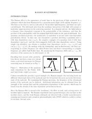
Figure 1-4: The <strong>easyScan</strong> 2 controller<br />
The Probe Status light<br />
Indicates the status of the Z-feedback loop. The Probe Status light can be in any of the<br />
following states:<br />
– Red<br />
The scanner is in its upper limit position. This occurs when the tip–sample interaction is<br />
stronger than the Setpoint for some time. There is danger of damaging the tip due to an<br />
interaction that is too strong.<br />
– Orange/yellow<br />
The scanner is in its lower limit position. This occurs when the tip–sample interaction is<br />
weaker than the Setpoint for some time. The tip is probably not in contact with the<br />
sample surface.<br />
– Green<br />
The scanner is not in a limit position, and the feedback loop is able to follow the sample<br />
surface.<br />
– Blinking green<br />
The feedback loop has been turned off in the software.<br />
17
CHAPTER 1: THE EASYSCAN 2 <strong>AFM</strong><br />
– Blinking red<br />
There is no laser signal with which to do feedback: see Section 9.3.1: Probe Status light<br />
blinks red (page 91) for possible causes and for more information on how to resolve this<br />
situation).<br />
The Scan Head lights<br />
Indicate the Scan Head type that is connected to the instrument. The Scan Head lights blink<br />
when no Scan Head can be detected, or when the controller has not been initialized yet.<br />
The Module lights<br />
Indicate the modules that are built in into the controller. The module lights blink when the<br />
controller has not been initialized yet. During initialization, the module lights are turned on<br />
one after the other.<br />
The Video Out connector<br />
An RCA/cinch connector that outputs a PAL video signal that can be connected to a video<br />
monitor.<br />
18
CHAPTER 2:<br />
Installing the <strong>easyScan</strong> 2<br />
<strong>AFM</strong><br />
0<br />
0
CHAPTER 2: INSTALLING THE EASYSCAN 2 <strong>AFM</strong><br />
2.1: Installing the hardware<br />
IMPORTANT<br />
• Make sure that the mains power connection is protected against excess voltage<br />
surges.<br />
• Place the instrument on a stable support in a location that has a low level of building<br />
vibrations, acoustic noise, electrical fields, and air currents.<br />
IMPORTANT<br />
• Never touch the cantilever tips, the cantilevers (Figure 1-2: Contents of the Tool set<br />
(page 15), item 10 and item 11), or any part of the Cantilever deflection detection<br />
system (Figure 3-2: Cantilever deflection detection system (page 30)).<br />
• Ensure that the surface to be measured is free of dust and possible residues.<br />
• Always put the Scan Head it in the Scan Head Case during transport and storage (see<br />
Figure 7-2: Scan Head storage).<br />
2.1.1: Installing the <strong>easyScan</strong> 2 controller<br />
1 Connect the USB Cable (Figure 1-1: Components (page 13), item 4) to the <strong>easyScan</strong> 2<br />
Controller (item 1), but do not connect it to the computer yet.<br />
IMPORTANT<br />
If you inadvertently connected the USB Cable to both the <strong>easyScan</strong> 2 Controller and a<br />
running computer, Windows will attempt to install drivers for the newly found<br />
hardware. When this happens, do the following:<br />
• Do NOT break off the installation!<br />
• Insert the Software Installation CD (if the Software Installation program should start,<br />
choose “Exit” first) and follow the steps described for the USB Video Adapter in Section<br />
2.2.4: Manual installation of the USB Video Adapter driver (page 25) to let Windows<br />
search for the necessary drivers on this CD.<br />
• When this process has finished, disconnect the USB cable from the computer, finish<br />
the remaining steps below, and then go through the Software Installation procedure<br />
as described in Section 2.2: Installing the SPM Control Software (page 23).<br />
20
INSTALLING THE HARDWARE<br />
2 Connect the Scan Head Cable (item 6) to the <strong>easyScan</strong> 2 controller but not to the Scan<br />
Head (item 2) yet.<br />
3 Connect the <strong>easyScan</strong> 2 Controller to the mains power using the Mains Cable (item 5),<br />
but do not turn on the controller yet.<br />
Figure 2-1: Measurement setup. Complete <strong>easyScan</strong> 2 <strong>AFM</strong> system with Sample Stage, Micrometer<br />
Translation Stage, <strong>AFM</strong> Video Module and Signal Module A.<br />
2.1.2: Installing the <strong>AFM</strong> Video Camera<br />
To install the <strong>AFM</strong> Video Camera:<br />
> Connect the Video Camera cable (Figure 1-1: Components (page 13), item 7) to the<br />
connector on the <strong>AFM</strong> Video Camera (Figure 1-1: Components (page 13), item 2) and to<br />
the Video In connector on the Controller (Figure 1-4: The <strong>easyScan</strong> 2 controller (page<br />
17)).<br />
To upgrade a system without Video Camera:<br />
1 Order the upgrade from your <strong>Nanosurf</strong> distributor.<br />
2 Send in the Scan Head and the Controller for mounting of the Video Camera on the<br />
Scan Head and installation of the Video Module inside the Controller.<br />
3 After the Controller has been returned, you should install the drivers for the <strong>AFM</strong> Video<br />
Module (Section 2.2: Installing the SPM Control Software).<br />
2.1.3: Installing the Signal Module S<br />
To install the Signal Module S:<br />
21
CHAPTER 2: INSTALLING THE EASYSCAN 2 <strong>AFM</strong><br />
> Connect the Break-out cable (Figure 1-1: Components (page 13), item 17) to the Signal<br />
Out connector on the Controller (Figure 1-4: The <strong>easyScan</strong> 2 controller (page 17)).<br />
In case of an upgrade, the Controller must be sent in to your local <strong>Nanosurf</strong> distributor for<br />
installing the Signal Module S electronics inside the Controller.<br />
2.1.4: Installing the Signal Module A and its Connector Box<br />
To install the Signal Module A:<br />
1 Connect one Signal Module cable (Figure 1-1: Components (page 13), item 19) to the<br />
Signal Out connector on the Controller and to the Output connector on the Signal<br />
Module A.<br />
2 Connect the other Signal Module cable to the Signal In connector on the Controller<br />
and to the Input connector on the Signal Module A.<br />
In case of an upgrade, the Controller must be sent in to your local <strong>Nanosurf</strong> distributor for<br />
installing the Signal Module A electronics in the Controller.<br />
2.1.5: Installing the <strong>easyScan</strong> 2 <strong>AFM</strong> Scan Head<br />
! WARNING<br />
LASER RADIATION (650nm)<br />
DO NOT STARE INTO THE BEAM<br />
OR VIEW DIRECTLY WITH OPTICAL<br />
INSTRUMENTS (MAGNIFIERS)<br />
CLASS 2M LASER PRODUCT<br />
• Always close the DropStop before inspecting or mounting a cantilever, or before<br />
inspecting the alignment chip, especially when using optical instruments (magnifiers)<br />
for the inspection.<br />
• Never remove the lens cover from the Scan Head (nor remove the built-in top view<br />
and side view lenses from the lens cover itself), as this would remove the optical filters<br />
that block back-reflected laser radiation and protect your eyes from laser damage.<br />
Older Scan heads may contain lasers with 850 nm wavelength infrared light, and lower<br />
optical power. These lasers have class 1 rating, which does not require special protection,<br />
even when viewing the laser radiation directly with optical instruments. The wavelength<br />
and laser class are indicated next to the serial number on the scan head (see Figure 1-3: Parts<br />
of the Scan Head (page 16)).<br />
22
INSTALLING THE SPM CONTROL SOFTWARE<br />
To mount the Scan Head<br />
1 Attach the Scan Head cable (Figure 1-1: Components (page 13), item 6) to the Scan<br />
Head (Figure 1-1: Components (page 13), item 2) using the screwdriver (Figure 1-2:<br />
Contents of the Tool set (page 15), item 4).<br />
The cable has a helix shape in order to isolate the Scan Head from vibrations of the<br />
table it is standing on. Take care that it is lying loosely on the table to ensure proper<br />
operation, and avoid stretching it.<br />
2 Place the Scan Head onto the <strong>AFM</strong> Sample Stage.<br />
It is recommended to cover the instrument in order to shield it from near-infrared light<br />
from artificial light sources, since this light may cause noise in the cantilever deflection<br />
detection system. The optional <strong>Nanosurf</strong> Scan Protector is optimized for this task, and<br />
additionally protects against noise and electrical interferences. Refer to the Scan Protector<br />
manual for instructions on how to set up and use the Scan Protector correctly.<br />
If the vibration isolation of your table is insufficient for your measurement purposes, use an<br />
active vibration isolation table such as the <strong>Nanosurf</strong> isoStage or the Halcyoncis_i4. Refer to<br />
the respective manuals for installation instructions.<br />
2.2: Installing the SPM Control Software<br />
2.2.1: Preparations before installing<br />
Before installation, the following steps need to be performed:<br />
1 Make sure the computer to be used meets the minimal computer requirements, as<br />
described in Chapter 11: Technical data under Computer requirements (page 103).<br />
2 When the <strong>easyScan</strong> 2 controller is connected to the computer via the USB cable,<br />
disconnect it by unplugging the USB cable from the computer.<br />
The <strong>easyScan</strong> 2 controller should only be connected to the computer when the<br />
controller software and driver installation is complete.<br />
3 Turn on the computer and start Windows.<br />
4 Log on to your computer with Administrator privileges.<br />
IMPORTANT<br />
Do not run any other programs while installing the <strong>easyScan</strong> 2 software.<br />
23
CHAPTER 2: INSTALLING THE EASYSCAN 2 <strong>AFM</strong><br />
2.2.2: Initiating the installation procedure<br />
To initiate the installation procedure:<br />
1 Insert the <strong>easyScan</strong> 2 Installation CD into the CD drive of the computer.<br />
In most cases, the Autorun CD Menu program will open automatically. Depending on<br />
your Autoplay settings, however, it is also possible that the Autoplay window opens,<br />
or that nothing happens at all. In these cases:<br />
> Click “Run CD_Start.exe” in the Autoplay window, or manually open the <strong>easyScan</strong><br />
2 Installation CD and start the program “CD_Start.exe”.<br />
IMPORTANT<br />
The <strong>easyScan</strong> 2 Installation CD contains calibration information (.hed files) specific to<br />
your instrument! Therefore, always store (a backup copy of) the CD delivered with the<br />
instrument in a safe place.<br />
2 Click the “Install <strong>easyScan</strong> 2 Software” button.<br />
The CD Menu program now launches the software setup program, which will start<br />
installation of all components required to run the <strong>Nanosurf</strong> <strong>easyScan</strong> 2 software.<br />
In Windows Vista/7, the User Account Control (UAC) dialog may pop up after clicking<br />
the “Install <strong>easyScan</strong> 2 Software” button, displaying the text “An unidentified program<br />
wants access to your computer”. If the name of the program being displayed is<br />
“Setup.exe”:<br />
> Click the “Allow” button.<br />
After the software setup program has started:<br />
1 Click “Next” in the “Welcome”, “Select Destination Folder”, and “Select Start Menu<br />
Folder” windows that sequentially appear, accepting the default choices in all dialogs.<br />
2 When the “Ready to install” window appears, click on the “Install” button.<br />
The setup program now performs its tasks without any further user interaction.<br />
Depending on the configuration of your computer, a reboot may be required at the<br />
end of the software installation process. If this is the case, the setup program will<br />
inform you of this, and will provide you with the opportunity to do so.<br />
This completes the software installation procedure. Proceed with Section 2.2.3: Hardware<br />
recognition to complete the setup process.<br />
24
INSTALLING THE SPM CONTROL SOFTWARE<br />
2.2.3: Hardware recognition<br />
To initiate the automatic hardware recognition process for the devices present in your<br />
<strong>easyScan</strong> 2 controller:<br />
1 Power on the <strong>easyScan</strong> 2 controller.<br />
2 Connect the <strong>easyScan</strong> 2 controller to the computer with the supplied USB cable (Figure<br />
1-1: Components (page 13), item 4).<br />
A popup balloon appears in the Windows notification area, stating that new hardware<br />
devices have been found and drivers are being installed. Depending on the<br />
configuration of your controller and computer, the detection process can take quite<br />
some time (20 seconds or more). Please be patient! After successful automatic<br />
installation, the popup balloon indicates that the installation has finished and that the<br />
devices are now ready for use.<br />
With some older <strong>easyScan</strong> 2 controllers, manual installation of the Video Adapter drivers<br />
will be required. This is indicated by the appearance of the “Found new Hardware” window<br />
during hardware recognition. The procedure to install the respective drivers manually<br />
differs slightly between Windows 2000/XP and Windows Vista/7, and is detailed in Section<br />
2.2.4: Manual installation of the USB Video Adapter driver. On controllers where manual<br />
installation of the USB Video Adapter driver is required, Hardware recognition and Manual<br />
installation of the USB Video Adapter driver should be repeated for each of the computer’s<br />
USB ports. It is recommended to do this now while you are logged on with Administrator<br />
privileges.<br />
This completes the hardware recognition process and the entire setup process. If you wish<br />
to use the Lithography features of the <strong>easyScan</strong> 2 software and want to design your own<br />
vector graphics for import into the lithography module, you can opt to install the<br />
LayoutEditor software by clicking the “Install CAD Program” button in the CD Menu<br />
program. This will launch the LayoutEditor installation program, which will guide you<br />
through the CAD program setup. Otherwise, you may exit now by clicking the “Exit” button.<br />
2.2.4: Manual installation of the USB Video Adapter driver<br />
If required for your controller, follow the operating-system-specific instructions below for<br />
manual installation of the Video Adapter driver. If Section 2.2.3: Hardware recognition (page<br />
25) was completed automatically, this section can be skipped.<br />
25
CHAPTER 2: INSTALLING THE EASYSCAN 2 <strong>AFM</strong><br />
Windows Vista/7<br />
To manually install the USB Video Adapter driver:<br />
1 In the “Found New Hardware” dialog for an “Unknown Device”, click the “Locate and<br />
install driver software (recommended)” button.<br />
The User Account Control (UAC) dialog may pop up after pressing this button,<br />
displaying the text “Windows needs your permission to continue” for a “Device driver<br />
software installation”. If this is the case:<br />
> Click the “Continue” button.<br />
2 In the next dialog, which states “Windows couldn’t find driver software for your<br />
device”, click the “Browse my computer for driver software (advanced)” button.<br />
3 In the next dialog, “Browse” to your CD drive (usually D:) or manually type “D:\” (or the<br />
corresponding drive letter) into the Path field. Make sure “include subfolders” is<br />
checked. Then click the “Next” button.<br />
Windows begins searching the specified path, and — since an unsigned driver is found<br />
— a Windows Security window opens, stating that “Windows can’t verify the publisher<br />
of this driver software”<br />
4 In the Windows Security window, click the “Install this driver software anyway” button.<br />
The Found New Hardware window now displays a “USB Video Adapter” and driver<br />
installation will take place.<br />
5 When Windows has finished installing the Video driver software, click “Close”.<br />
Windows 2000/XP<br />
To manually install the USB Video Adapter driver:<br />
1 When the “Found New Hardware” dialog displays the text “Can Windows connect to<br />
Windows Update to search for software?”, select “No, not this time” and click “Next”.<br />
2 In the next dialog, select “Install automatically (recommended)” and click “Next”.<br />
Windows now begins searching for the appropriate driver, and — since an unsigned<br />
driver is found — a Warning window opens, stating that “The software that you are<br />
trying to install for this hardware: USB Video Adapter has not passed Windows Logo<br />
testing for compatibility with Windows XP”.<br />
3 In the Warning window, click the “Continue anyway” button.<br />
Under some circumstances a “Files Needed” window may pop up. If this is the case:<br />
> “Browse” to the Installation CD’s “DriverVideo” folder and click “OK”.<br />
4 When Windows has finished installing the Video driver, click “Finish”.<br />
26
CHAPTER 3:<br />
Preparing for<br />
measurement<br />
0<br />
0
CHAPTER 3: PREPARING FOR MEASUREMENT<br />
3.1: Introduction<br />
Once the system has been set up (see Chapter 2: Installing the <strong>easyScan</strong> 2 <strong>AFM</strong> (page 19)),<br />
the instrument and the sample have to be prepared for measurement. The preparation<br />
consists of three steps: Initializing the <strong>easyScan</strong> 2 Controller, Installing the cantilever, and<br />
Installing the sample.<br />
3.2: Initializing the <strong>easyScan</strong> 2 Controller<br />
To initialize the <strong>easyScan</strong> 2 controller:<br />
1 Make sure that the <strong>easyScan</strong> 2 controller is connected to the mains power and to the<br />
USB port of the control computer.<br />
2 Turn on the power of the <strong>easyScan</strong> 2 controller.<br />
First all status lights on top of the controller briefly light up. Then the Scan Head lights<br />
and the lights of the detected modules will start blinking, and all other status lights<br />
turn off.<br />
3 Start the SPM Control Software on the control computer.<br />
The main program window appears, and all status lights are turned off. Now a Message<br />
“Controller Startup in progress” is displayed on the computer screen, and the module<br />
lights are turned on one after the other. When initialization is completed, a Message<br />
“Starting System” is briefly displayed on the computer screen, and the Probe Status<br />
light, the Scan Head status light of the detected scan head, and the Module lights of<br />
the detected modules will light up. If no scan head is detected, both Scan Head Status<br />
lights blink.<br />
4 In the Preparation group of the Acquisition tab you will see the currently selected<br />
<strong>Operating</strong> mode and Cantilever type.<br />
5 Determine which operating mode you wish to use.<br />
Refer to Chapter 6: <strong>Operating</strong> modes (page 66) for the properties of the modes<br />
available.<br />
To change the operating mode:<br />
28
INSTALLING THE CANTILEVER<br />
> Select the desired operating mode from the <strong>Operating</strong> mode drop-down menu<br />
by clicking the currently selected operating mode:<br />
6 Determine which cantilever type you wish to use.<br />
The cantilever suited for your measurements will depend on Measurement<br />
environment, the selected <strong>Operating</strong> mode and on your sample.<br />
To change the cantilever type:<br />
> Select the desired cantilever type from the Cantilever type drop-down menu by<br />
clicking the currently selected cantilever type:<br />
3.3: Installing the cantilever<br />
To maximize ease of use, the <strong>easyScan</strong> 2 <strong>AFM</strong> is designed in such a way that the cantilever<br />
can quickly be installed and removed without having to re-adjust the cantilever deflection<br />
detection system. The quick cantilever installation is possible because the Scan Head<br />
contains a self-alignment system. The alignment system consists of a structure in the<br />
alignment chip and matching grooves in the back side of the cantilever chip. The alignment<br />
system positions the cantilever with micrometer accuracy (see Figure 3-1: Cantilever, left).<br />
This accuracy is only guaranteed when the cantilever and the mounting chip are absolutely<br />
clean. Installation of the cantilever should therefore still be carried out with great care. The<br />
quality of measurements depends strongly on the accuracy of the installation.<br />
29
CHAPTER 3: PREPARING FOR MEASUREMENT<br />
Figure 3-1: Cantilever. (Left) Alignment system. (Center) Cantilever chip viewed from the top. (Right)<br />
Cantilever, 450 μm long, 50 μm wide with integrated tip.<br />
Sample illumination<br />
Cantilever<br />
Photodetector<br />
Cantilever<br />
holder spring<br />
Laser<br />
Alignment chip<br />
Hole for cantilever<br />
insertion tool<br />
Figure 3-2: Cantilever deflection detection system<br />
3.3.1: Selecting a cantilever<br />
It is very important that the cantilever type is suitable for the operating mode that is used.<br />
Stiffer and shorter cantilevers (e.g. NCLR, Nanoworld or Tap190Al-G, BudgetSensors) are<br />
generally used for the Dynamic operating mode. More flexible and longer cantilevers (e.g.<br />
CONTR, Nanoworld or ContAl-G, BudgetSensors) are generally used for the Static operating<br />
mode.<br />
To change to a different cantilever type:<br />
> In the Preparation group of the Acquisition tab, select the desired cantilever type from<br />
the “Mounted cantilever” drop-down menu by clicking the currently selected<br />
cantilever type.<br />
The various usable types are listed in Section 11.2.1: Specifications and features (page 100),<br />
under Compatible cantilevers.<br />
30
INSTALLING THE CANTILEVER<br />
3.3.2: Inserting the cantilever in the Scan Head<br />
! WARNING<br />
LASER RADIATION (650nm)<br />
DO NOT STARE INTO THE BEAM<br />
OR VIEW DIRECTLY WITH OPTICAL<br />
INSTRUMENTS (MAGNIFIERS)<br />
CLASS 2M LASER PRODUCT<br />
• Always close the DropStop before inspecting or mounting a cantilever, or before<br />
inspecting the alignment chip, especially when using optical instruments (magnifiers)<br />
for the inspection.<br />
• Never remove the lens cover from the Scan Head (nor remove the built-in top view<br />
and side view lenses from the lens cover itself), as this would remove the optical filters<br />
that block back-reflected laser radiation and protect your eyes from laser damage.<br />
Older Scan heads may contain lasers with 850 nm wavelength infrared light, and lower<br />
optical power. These lasers have class 1 rating, which does not require special protection,<br />
even when viewing the laser radiation directly with optical instruments. The wavelength<br />
and laser class are indicated next to the serial number on the scan head (see Figure 1-3: Parts<br />
of the Scan Head (page 16)).<br />
CAUTION<br />
• Nothing should ever touch the cantilever.<br />
• The Cantilever Holder Spring is very delicate. NEVER touch or pull on it! It will become<br />
bent and unusable otherwise!<br />
• Always close the DropStop before handling the cantilever. If you fail to do so, the<br />
cantilever can fall into the Scan Head, causing malfunction of the microscope,<br />
particularly of the scanner.<br />
• If a cantilever has dropped into the Scan Head, and the microscope is malfunctioning,<br />
contact your local support. Never open the Scan Head, because this will cause<br />
damage to the scanner and the laser beam deflection detection system.<br />
To remove the old cantilever:<br />
1 Put the Scan Head upside-down on the table.<br />
31
CHAPTER 3: PREPARING FOR MEASUREMENT<br />
2 Remove the Cantilever Insertion Tool from the DropStop<br />
3 Close the DropStop (see Figure 3-3: Closing the DropStop).<br />
The laser beam is now blocked by the DropStop. As a consequence, the Probe Status<br />
light on the <strong>easyScan</strong> 2 controller will now blink red.<br />
4 Place the cantilever insertion tool (Figure 1-2: Contents of the Tool set (page 15), item 5)<br />
into the hole behind the alignment chip (Figure 3-4: Mounting the cantilever, top left).<br />
The Cantilever Holder Spring opens.<br />
5 Use the Cantilever Tweezers (figure Figure 1-2: Contents of the Tool set (page 15), item<br />
3) to remove the old cantilever from the instrument (Figure 3-4: Mounting the cantilever,<br />
top right).<br />
CAUTION<br />
Always store and ship the Scan Head with a cantilever installed. Otherwise, the<br />
cantilever holder spring may damage the alignment chip.<br />
Figure 3-3: Closing the DropStop<br />
To insert the new cantilever:<br />
1 Take the new cantilever out of its box with the cantilever tweezers.<br />
2 Place the cantilever carefully on the alignment chip in the Scan Head (Figure 3-4:<br />
Mounting the cantilever, top right).<br />
3 Verify that the cantilever does not move with respect to the Alignment Chip by<br />
carefully tapping on it with the tweezers.<br />
If the cantilever does move, it is probably not inserted correctly. Refer to Figure 3-5:<br />
Cantilever Alignment for correct alignment and examples of incorrect alignment.<br />
4 Gently pull the cantilever insertion tool out of the hole.<br />
The Cantilever Holder Spring closes and holds the cantilever chip tightly in position<br />
(Figure 3-4: Mounting the cantilever, bottom right).<br />
32
INSTALLING THE CANTILEVER<br />
Figure 3-4: Mounting the cantilever. (top left) inserting the cantilever insertion tool, (top right)<br />
inserting/removing the cantilever, (bottom right) correctly inserted cantilever.<br />
Figure 3-5: Cantilever Alignment. (Left) correct: the mirrored environment shows a reflection that is<br />
continuous over the cantilever and the alignment chip, and small triangular gaps can be seen between<br />
the edges of the alignment chip and the corners of the cantilever chip, (center & right) incorrect: the<br />
mirrored environment shows a reflection that is different on the cantilever and on the alignment chip,<br />
and no nice triangular gaps can be discerned.<br />
5 Remove the DropStop.<br />
The laser beam is now unblocked, and the Probe Status light on the <strong>easyScan</strong> 2<br />
controller should now stop blinking red. If this is not the case refer to Section 9.3.1:<br />
Probe Status light blinks red (page 91).<br />
33
CHAPTER 3: PREPARING FOR MEASUREMENT<br />
3.4: Installing the sample<br />
3.4.1: Preparing the sample<br />
The <strong>easyScan</strong> 2 <strong>AFM</strong> can be used to examine any material with a surface roughness that<br />
does not exceed the height range of the scanning tip. Nevertheless the choice and<br />
preparation of the surface can influence the surface–tip interaction. Examples of<br />
influencing factors are excess moisture, dust, grease or other contaminations of the sample<br />
surface. Because of this, some samples need special preparation to clean their surface.<br />
Generally, however, only clean your samples if this is absolutely required, and be sure to<br />
clean very carefully in order not to harm the sample surface.<br />
If the surface is dusty, try to measure on a clean area between the dust. Although it is<br />
possible to blow away coarse particles with dry, oil-free air, small particles generally stick<br />
quite strongly to the surface and cannot be easily removed this way. Also note that bottled,<br />
pressurized air is generally dry, but pressurized air from an in-house supply is generally not.<br />
In this case an oil filter should be installed. Blowing away dust by breath is not advisable,<br />
because it too is not dry, and the risk of contaminating the sample even further is very high.<br />
When the sample surface is contaminated with solid matter or substances that can be<br />
dissolved, the surface should be cleaned with a solvent. Suitable solvents are distilled or<br />
demineralized water, alcohol or acetone, depending on the nature of the contaminant. The<br />
solvent should always be highly pure in order to prevent accumulation of impurities<br />
contained within the solvent on the sample surface. When the sample is very dirty, it should<br />
be cleaned several times to completely remove partially dissolved and redeposited<br />
contaminants. Delicate samples, which would suffer from such a treatment, can<br />
alternatively be cleaned in an ultrasonic bath.<br />
3.4.2: <strong>Nanosurf</strong> samples<br />
<strong>Nanosurf</strong> delivers various optional samples, which are usually packed in the <strong>AFM</strong> Tool Set.<br />
These samples are briefly described here. Further samples are available in the <strong>AFM</strong><br />
Extended Sample Kit, which contains its own sample description.<br />
All samples should be stored in their respective box. This way, it should not be necessary to<br />
clean them. Cleaning of the samples is generally not advisable (unless indicated below),<br />
because their surfaces are often rather delicate.<br />
Grid: 10 μm / 100 nm<br />
The Grid: 10 μm / 100 nm can be used for testing the XY-calibration of the 70 μm and<br />
100 μm scanners, and for testing the Z-calibration. It is manufactured using standard silicon<br />
34
INSTALLING THE SAMPLE<br />
100 nm<br />
Figure 3-6: Structure of Grid: 10 μm / 100 nm<br />
microfabrication technology, which produces silicon oxide squares on a silicon substrate. It<br />
has a period of 10 μm and a square height of approximately 100 nm.<br />
Sample specifications:<br />
Size:<br />
5 mm × 5 mm<br />
Material:<br />
Silicon oxide on silicon<br />
Structure:<br />
Square array of square hills of silicon oxide hills on silicon.<br />
Grid period:<br />
10 μm<br />
Approximate height: 100 nm<br />
Calibrated values of period and height (with 3% accuracy) are printed on the package.<br />
Certified Calibration grids are available as an option.<br />
Grid: 660 nm<br />
10 µm<br />
The Grid: 660 nm can be used to test the XY-calibration of the 10 μm scanner. Depending<br />
on the grid version, it consists either of:<br />
• Silicon oxide hills on a silicon substrate with a period of 660 nm and an unspecified<br />
height. The approximate height is 149 nm,<br />
• Holes in a silicon oxide layer with a period of 660 nm and an unspecified depth. At the<br />
time of writing, the approximate depth is 60 nm.<br />
35
CHAPTER 3: PREPARING FOR MEASUREMENT<br />
Sample specifications:<br />
Size: 5 mm × 5 mm<br />
Material: Silicon oxide on silicon<br />
Structure: Square array of holes or hills in the silicon oxide layer<br />
Period:<br />
660 nm. Calibrated value of period (with 3% accuracy) is printed on the<br />
package. Certified Calibration grids are available as an option.<br />
60 nm<br />
Figure 3-7: Structure of Grid: 660nm (version with holes)<br />
Flatness sample<br />
The Flatness sample is a polished silicon sample. It can be used for testing the Flatness of<br />
the scanned plane.<br />
Sample specifications:<br />
Size: 5 mm × 5 mm<br />
Material: Silicon<br />
Thickness: Approx. 320 μm<br />
CD-ROM piece<br />
Sample for demonstrating the <strong>AFM</strong> imaging. The CD sample is a piece from a CD, without<br />
any coating applied to it.<br />
Sample specifications:<br />
Material:<br />
Structure:<br />
Microstructure<br />
660 nm<br />
Polycarbonate<br />
100 nm deep pits arranged in tracks that are spaced 1.6 μm apart.<br />
Sample for demonstrating <strong>AFM</strong> imaging (no longer available). The microstructure is<br />
approximately the negative of the Grid: 10μm / 100nm. It consists of holes in a silicon oxide<br />
36
INSTALLING THE SAMPLE<br />
layer with an unspecified period and depth. The approximate period is 10 μm, the<br />
approximate depth is 100 nm.<br />
Graphite (HOPG) on sample support<br />
This sample can be used for STM as well as <strong>AFM</strong> measurements. In high resolution <strong>AFM</strong><br />
measurements, the atomic steps of the graphite surface can be seen. Conductivity<br />
variations can be observed in Spreading Resistance mode.<br />
Sample specifications:<br />
Size:<br />
5 mm × 5 mm<br />
Material:<br />
Highly Oriented Pyrolytic Graphite (HOPG)<br />
Sample support: Magnetic Steel disc, galvanized with Nickel.<br />
The surface of the graphite sample can be cleaned when it is very dirty or uneven. Due to<br />
the layered structure of graphite this can easily be done using a piece of adhesive tape<br />
(Figure 3-8: Cleaving graphite):<br />
1 Put the sample on the table using a pair of tweezers.<br />
2 Stick a piece of adhesive tape gently to the graphite and then pull it off again.<br />
The topmost layer of the sample should stick to the tape.<br />
3 Remove any loose flakes with the tweezers.<br />
The graphite sample is now ready for use and should not be touched anymore.<br />
Figure 3-8: Cleaving graphite<br />
3.4.3: Stand-alone measurements<br />
You can either use the instrument with a sample stage, or as a stand-alone instrument. The<br />
sample stage offers vibration isolation, and a stable scan head mount. Therefore, only<br />
operate the instrument as a stand-alone when the sample is too large for the sample stage.<br />
37
CHAPTER 3: PREPARING FOR MEASUREMENT<br />
For stand-alone measurements, put the Scan head directly on top of the sample. Protection<br />
feet to be placed under the three alignment screws are provided to protect delicate<br />
samples from being scratched (Figure 1-2: Contents of the Tool set (page 15), item 2).<br />
3.4.4: The Sample Stage<br />
The Sample Stage (Figure 1-1: Components (page 13), item 8) offers vibration isolation and<br />
reproducible scan head placement (see Figure 3-9: The <strong>easyScan</strong> 2 <strong>AFM</strong> Scan Head on its<br />
Sample Stage), and can be used to comfortably position a sample. An optional Micrometer<br />
Translation Stage for XY-positioning can be mounted on the Sample Stage. The sample can<br />
either be put directly on the sample stage, or mounted onto the Sample Holder (Figure 1-2:<br />
Contents of the Tool set (page 15), item 7) before measurement (see Section 3.4.5: Mounting<br />
a sample).<br />
Figure 3-9: The <strong>easyScan</strong> 2 <strong>AFM</strong> Scan Head on its Sample Stage<br />
3.4.5: Mounting a sample<br />
Samples may either be placed directly onto the sample stage, or first mounted onto the<br />
Sample Holder before being placed there.<br />
To mount a sample onto the Sample Holder:<br />
1 Put a double-sided adhesive tape on the frontside of a Post-it ® note, so that it is on the<br />
opposite side of the sticky part.<br />
2 Cut off all parts of the note that do not have adhesive tape on it.<br />
3 Fix the tape-side of the prepared note to the Sample Holder.<br />
38
INSTALLING THE SAMPLE<br />
Figure 3-10: Sample mounted onto the Sample Holder<br />
4 Put the sample on the sticky side of the Post-it ® note, and press on it lightly.<br />
The result should resemble Figure 3-10: Sample mounted onto the Sample Holder.<br />
5 Remove the scan head and place the Sample Holder on top of the Sample plate.<br />
It is recommended to always connect the Sample Holder to the ground connector on<br />
the Scan Head using the ground cable.<br />
6 Place the scan head back onto the Sample Stage, but be sure to keep a safe distance<br />
between the cantilever and the sample surface. If necessary, adjust the tip–sample<br />
distance via the leveling screws before placing back the scan head.<br />
39
40<br />
CHAPTER 3: PREPARING FOR MEASUREMENT
CHAPTER 4:<br />
A first measurement<br />
0<br />
0
CHAPTER 4: A FIRST MEASUREMENT<br />
4.1: Introduction<br />
In this chapter, step-by-step instructions are given to operate the microscope and to<br />
perform a simple measurement. More detailed explanations of the software and of the<br />
system can be found elsewhere in this manual.<br />
4.2: Running the microscope simulation<br />
The SPM Control Software can be started without having the microscope connected to<br />
your computer in order to explore the <strong>easyScan</strong> 2 system (measurements and software)<br />
without danger of damaging the instrument or the cantilever. In simulation mode, most<br />
functions of the real microscope are emulated. The sample is replaced by a mathematical<br />
description of a surface.<br />
When the SPM Control Software is started without a microscope connected to your<br />
computer, the following dialog appears:<br />
> Click “OK”.<br />
The status bar will now display the text “Simulation”.<br />
You can also switch to simulation mode with the microscope connected:<br />
> In the Hardware group of the Settings tab, click the “Simulation” button.<br />
The “Simulation” button will now be highlighted and the status bar will display the text<br />
“Simulation”.<br />
To exit the microscope Simulation mode:<br />
> In the Hardware group of the Settings tab, click the “Simulation” button again.<br />
The highlighting of the “Simulation” button will now disappear, and the status bar will<br />
display the text “Online”.<br />
42
PREPARING THE INSTRUMENT<br />
4.3: Preparing the instrument<br />
IMPORTANT<br />
• Never touch the cantilever or the surface of the sample! Good results rely heavily on a<br />
correct treatment of the tip and the sample.<br />
• Avoid exposing the system to direct light while measuring. This could influence the<br />
cantilever deflection detection system and reduce the quality of the measurement.<br />
Prepare the instrument as follows (see Chapter 3: Preparing for measurement (page 27) for<br />
more detailed instructions):<br />
1 If you have the <strong>AFM</strong> Dynamic Module, install an NCLR type cantilever, otherwise install<br />
a CONTR type cantilever.<br />
2 Install one of the samples from the <strong>Nanosurf</strong> <strong>AFM</strong> Basic Sample Kit or Calibration<br />
Sample Kit. Preferably, install the 10 μm Calibration grid when using a 70-μm or 110-<br />
μm scan head, and the 660 nm Calibration grid when using a 10-μm scan head.<br />
The measurement examples shown here were made with the 10 μm Calibration grid.<br />
To make sure that the configuration is correct, do the following:<br />
1 Open the menu item “File” >> “Parameters” >> “Load...”, and load the file “Default_EZ2-<br />
<strong>AFM</strong>.par” from the directory that holds the default <strong>easyScan</strong> 2 configurations.<br />
Usually this is “C:\Program Files\<strong>Nanosurf</strong>\Nansurf <strong>easyScan</strong> 2\Config”.<br />
2 Open the menu item “File” >> “Chart Arrangement” >> “Load...”, and load the file<br />
“Default_EZ2-<strong>AFM</strong>.chart” from the directory that holds the default <strong>easyScan</strong> 2<br />
configurations.<br />
4.3.1: Entering and changing parameter values<br />
Parameter values can be found in the parameter sections of the <strong>Operating</strong> windows and in<br />
special dialogs. Depending on your measurement or optimization thereof, you may from<br />
time to time need to change or enter new values.<br />
To change a parameter or enter a value:<br />
1 Activate the parameter by clicking inside the (white) parameter edit box with the<br />
mouse:<br />
43
CHAPTER 4: A FIRST MEASUREMENT<br />
2 In case of a drop-down menu selection list, change the selection using the mouse or<br />
the up and down arrows on the keyboard. In case of a numerical value, use one of the<br />
following methods:<br />
• Use the up and down arrow keys on the keyboard to increase or decrease its value.<br />
The new value is automatically used after one second.<br />
• Click the arrow buttons next to the parameter value with the mouse pointer.<br />
Normally, the parameter value is changed by a small amount (usually in the range of<br />
1–10%). Some edit boxes are doubling or dividing the parameter value by two (e.g.<br />
the “points/line” parameter). The new value is automatically used after one second.<br />
• Enter the new value using the keyboard. The entered value is applied upon pressing<br />
the “Enter” or “Return” key, or by activating another input. The entered value is<br />
discarded upon pressing the “Esc” key. The unit prefix can be changed by typing one<br />
of the following keyboard keys:<br />
f = femto space bar = no prefix<br />
p = pico k = kilo<br />
n = nano M (shift-m) = mega<br />
u = micro G (shift-g) = giga<br />
m = milli T (shift-t) = tera<br />
Examples: if the basic unit is Volts, type “m” to change to millivolts, type the space<br />
bar for volts, type “u” for microvolts.<br />
Sometimes the program will change an entered value to a slightly different value. This<br />
happens when the desired value is outside the digitization range of the <strong>easyScan</strong> 2<br />
controller, for example due to resolution or timing limits. In such cases, the desired<br />
value is automatically changed to the nearest possible value.<br />
4.4: Approaching the sample<br />
To start measuring, the cantilever tip must come within a fraction of a nanometer of the<br />
sample without touching it with too much force. To achieve this, a very careful and sensitive<br />
approach of the cantilever is required. This delicate operation is carried out in three steps:<br />
Manual coarse approach, Manual approach using the motorized approach stage, and the<br />
Automatic final approach. The color of the Status light on the controller shows the current<br />
status of the approach:<br />
– Orange/yellow<br />
Normal state during approach: the Z-scanner is fully extended toward the sample.<br />
– Red<br />
The approach has gone too far: the tip was driven into the sample, and the Z-scanner is<br />
fully retracted from the sample. In this case, the tip is probably damaged and you will<br />
have to install a new cantilever again.<br />
44
APPROACHING THE SAMPLE<br />
– Green<br />
The approach has finished successfully: the Z-scanner is within the measuring range.<br />
To prepare for the approach process:<br />
> Select the Acquisition tab<br />
The controls for positioning the cantilever with respect to the sample are located in the<br />
Approach group.<br />
During the approach steps described in the following sections, use the side view of the<br />
cantilever to judge the distance between tip and sample surface:<br />
> If the <strong>AFM</strong> Video Camera is installed, select “Side view” in the Video panel located in<br />
the Info pane (see Section 13.6: Video panel (page 135)).<br />
If the Video Camera is not installed, use the side view lens of the scan head to observe<br />
the sample instead.<br />
4.4.1: Manual coarse approach<br />
In this step, the sample surface is brought within the range of the motorized approach<br />
stage of the Scan Head.<br />
To perform a manual coarse approach:<br />
> Use the three leveling screws to lower the Scan head so that the cantilever is within 1–<br />
2 mm of the sample (see Figure 1-3: Parts of the Scan Head (page 16)). Take care that the<br />
Scan head remains parallel to the sample surface by approximately turning all screws<br />
equally.<br />
The side view should now look as shown in Figure 4-1: Side view of the cantilever after<br />
manual coarse approach. When the sample is reflective, the mirror image of the<br />
cantilever should be visible. When the sample is not reflective, the shadow of the<br />
cantilever may be visible. If neither a mirror image nor a shadow is visible, change the<br />
environment light until it is. You can use the cantilever as a ruler to judge distances in<br />
the views of the integrated optics.<br />
45
CHAPTER 4: A FIRST MEASUREMENT<br />
Figure 4-1: Side view of the cantilever after manual coarse approach.<br />
4.4.2: Manual approach using the motorized approach stage<br />
In this step, the tip is brought as close to the sample surface as possible, without touching<br />
it. The closer the two are together, the less time the automatic final approach takes.<br />
1 Observe the distance between tip and sample in the side view of the integrated optics.<br />
Figure 4-2: View of sample and cantilever after manual approach using the motorized approach<br />
stage. (Left) side view, (Right) top view.<br />
46
APPROACHING THE SAMPLE<br />
2 While observing the tip–sample distance, click and hold the “Advance” button in the<br />
Approach group of the Acquisition tab until the tip is close enough to the sample:<br />
The tip should not come closer to the sample than a few times the cantilever width<br />
(Figure 4-2: View of sample and cantilever after manual approach using the motorized<br />
approach stage, left).<br />
Now that the sample is in focus, the top view image can be used to find a suitable location<br />
to measure on. In top view, the sample is seen from a direction perpendicular to its surface<br />
(see Figure 4-2: View of sample and cantilever after manual approach using the motorized<br />
approach stage, right).<br />
To use the top view:<br />
1 If the <strong>AFM</strong> Video Camera is installed, select Top view in the Video panel (see Section<br />
13.6: Video panel (page 135)). If the Video Camera is not installed, use the top view lens<br />
to observe the sample instead.<br />
2 If necessary, move the Sample Holder to find a suitable location that is free of dust<br />
particles.<br />
4.4.3: Automatic final approach<br />
In this last step, the tip automatically approaches the sample until a given Setpoint is<br />
reached. Before starting the automatic approach, select the desired operating mode and<br />
cantilever type. To do this:<br />
> In the Preparation group of the Acquisition tab, select an operating mode and<br />
cantilever type that match the cantilever installed.<br />
In Dynamic Force mode, the instrument will automatically determine the vibration<br />
frequency to be used during imaging. To determine the optimal frequency, the controller<br />
performs a coarse and a fine frequency sweep in which the cantilever vibration amplitude<br />
(and — in Phase Contrast mode — also the phase) are recorded as a function of excitation<br />
47
CHAPTER 4: A FIRST MEASUREMENT<br />
frequency. It is instructive to see both frequency sweep measurements in all detail at least<br />
once. To do this, it is possible to manually perform the frequency sweeps:<br />
1 In the Preparation group of the Acquisition tab, click the “Freq. Sweep” button:<br />
The Vibration Frequency Search dialog now opens (see Section 17.11: Vibration<br />
Frequency Search dialog (page 239) for details).<br />
2 Click the “Auto frequency set” button.<br />
The SPM Control Software now sets appropriate values for the coarse and fine sweeps<br />
and performs these sweeps. The fine sweep will overwrite the data of the coarse<br />
sweep in the charts displayed in the “Vibration frequency search” dialog. To see the<br />
results of the individual sweeps:<br />
> Press the “Coarse sweep” and “Fine sweep” buttons sequentially.<br />
Before final approach of the sample, it is necessary to set the scanning and feedback<br />
parameters of the control software to suitable initial values. The easiest way to do this is to<br />
use the “Auto Set” wizard:<br />
1 In the Preparation group of the Acquisition tab, click the “Auto Set” button:<br />
A dialog will pop up, which will ask you some basic questions about your sample and<br />
your measurement needs.<br />
2 Answer the questions of the wizard to the best of your knowledge.<br />
For descriptions of the features of standard <strong>Nanosurf</strong> samples refer to Section 3.4.2:<br />
<strong>Nanosurf</strong> samples (page 34).<br />
Now that the initial software settings have been given suitable values, you need to name<br />
the measurement series (see Section 16.4.1: History File mask (page 182)). Each completed<br />
measurement (scan/image) will be temporarily saved (automatically) in the History folder<br />
under this name, with index numbers (or, optionally, date and time attributes) added to<br />
identify the individual measurements. It is best to enter the measurement series’ name<br />
now, since the control software will (by default) start measuring as soon as the final<br />
approach is done. It is also strongly recommended to move all relevant measurements to a<br />
48
STARTING A MEASUREMENT<br />
new folder when you are finished, since the files in the History folder will be overwritten<br />
over time (see Max History Files (page 211)).<br />
To set the measurement series name:<br />
1 Activate the Gallery panel (see Section 16.4: Gallery panel (page 181)) in the Info pane.<br />
2 Click the History tab at the top of the Gallery panel with the mouse.<br />
3 In the entry box at the top of the panel, enter a name by hand or use the Mask Editor<br />
dialog (see Section 16.4.4: Mask Editor dialog (page 183)) to create the name mask.<br />
If no [INDEX] attribute is explicitly added to the name mask, it will be implicitly applied<br />
to the end of the file name so that individual measurements can be stored and<br />
distinguished.<br />
The automated final approach can now be started. To do this:<br />
1 In the Approach group of the Acquisition tab, click the “Approach” button:<br />
The cantilever is moved towards the sample via the approach stage, with the Z-<br />
Controller turned on. This movement continues until the Z-Controller error becomes<br />
zero. From this point onward, the distance between sample and tip is maintained<br />
automatically by the electronics. The probe status light changes to a constant green,<br />
and a message “Approach done” appears:<br />
2 Click the “OK” button.<br />
If the automatic final approach fails, refer to Section 9.3: <strong>AFM</strong> measurement problems (page<br />
91) for the next steps to take.<br />
4.5: Starting a measurement<br />
Now that the tip–sample interaction defined by Setpoint is established between tip and<br />
sample, measurements can start. By default, the instrument is set to automatically start<br />
measuring after the automatic approach. If this is not the case:<br />
49
CHAPTER 4: A FIRST MEASUREMENT<br />
> Start measurements manually by clicking the “Start” button in the Imaging group of<br />
the Acquisition tab:<br />
Two representations of the ongoing measurement are drawn in the Imaging panel. One<br />
representation is a color coded height image (Topography) called a Color map. The other is<br />
a plot of height as a function of X* position called a Line graph. With the current settings,<br />
the software automatically adjusts the contrast of the Color map, and height range of the<br />
Line graph to the data that have been measured.<br />
To judge the imaging quality, watch the displays until at least one fourth of the<br />
measurement has been completed.<br />
IMPORTANT<br />
Measurements on the micrometer/nanometer scale are very sensitive to environment<br />
influences. Direct light or fast movements — causing air flow and temperature<br />
variations near the Scan Head — can influence and disturb the measurement.<br />
When a measurement contains large disturbances, or no two scan lines are similar, stop<br />
measuring and reduce or eliminate the disturbances. To do this:<br />
> Click the “Stop” button in the Imaging group of the Acquisition tab and follow the<br />
instructions in Chapter 9: Problems and solutions (page 87):<br />
4.6: Selecting a measurement area<br />
If you were able to prepare your measurement so that the scan line in the Line graph<br />
reproduces stably, the color map graph should look similar to the one shown below after<br />
the measurement has finished.<br />
To zoom in to an interesting part of the measurement:<br />
1 Activate the color map graph by clicking on it.<br />
50
SELECTING A MEASUREMENT AREA<br />
Figure 4-3: Zooming in on an overview measurement<br />
2 Click the “Zoom” button in the Chart bar:<br />
The mouse pointer becomes pen-shaped when moving over the color map.<br />
3 Click on one corner of the region to be selected using the left mouse button, and keep<br />
the button pressed.<br />
4 Drag the mouse to the other corner of the region.<br />
The size and the position of the square are shown in the Tool results panel of the Info<br />
pane.<br />
5 Release the mouse button when the size of the square covers approximately one<br />
period of the grid.<br />
6 Confirm the selection by double clicking the color map graph using the left mouse<br />
button. Now the selection is enlarged to the whole display size. You can abort the<br />
zoom function by clicking the “Zoom” button again.<br />
The microscope will now start measuring a single grid period. Once the measurement is<br />
completed, you should get an image such as the one in Figure 4-4: Zoomed measurement,<br />
left. The depression in the sample surface to the sides of the structure is due to the LineFit<br />
data filter used. To remove it, click on “LineFit” and select the data filter “Raw Data” from the<br />
drop-down menu. The chart will now look like Figure 4-4: Zoomed measurement, right.<br />
51
CHAPTER 4: A FIRST MEASUREMENT<br />
Figure 4-4: Zoomed measurement. (Left) with line subtraction, (Right) without line subtraction.<br />
4.7: Storing the measurement<br />
By default, each completed measurement is temporarily stored (automatically) on your<br />
computer so that it can be used later. Additionally, you can also take snapshots of<br />
measurements still in progress. To do this:<br />
> Click the “Capture” button in the Chart bar:<br />
The current measurement is immediately stored and will show up in the History page<br />
of the Gallery panel, together with all other finished/stored measurements (see Section<br />
16.4: Gallery panel (page 181) for details). In addition, the captured document will<br />
remain open in the Document space of the SPM Control Software.<br />
Measurement documents in the temporary History folder should always be moved to a<br />
new location for permanent storage when you are done measuring. For details on how to<br />
do this, see Save as (page 182). Measurement documents thus permanently stored can<br />
always be loaded with the SPM Control Software or the optional <strong>Nanosurf</strong> Report or<br />
<strong>Nanosurf</strong> Analysis software packages for later viewing, analysis, and printing. A brief<br />
introduction on how to create a basic report using the Report software is given in the next<br />
section. For more detailed information on starting and using the Report software, see<br />
Section 22.2: Creating a report (page 452), or refer to the <strong>Nanosurf</strong> Report online help.<br />
52
CREATING A BASIC REPORT<br />
4.8: Creating a basic report<br />
The optional <strong>Nanosurf</strong> Report software can be used to evaluating the measurement, and<br />
to create visually appealing reports. Here, we will just start the software and create a basic<br />
report.<br />
To create a basic report of a completed measurement:<br />
1 Open a measurement from the Gallery panel.<br />
2 In the Report group of the Analysis tab, click the “Report” button.<br />
The <strong>Nanosurf</strong> Report software will now launch, import the currently open<br />
measurement, and evaluate the data using the default template.<br />
IMPORTANT<br />
After a fresh installation of the Report software, the Report software has to be run at least<br />
once before it can be automatically started from within the SPM Control Software. To run<br />
the Report software for the first time, select it from the Microsoft Windows “Start” menu.<br />
4.9: Further options<br />
From this point on, there are several things that can be done. Please refer to the respective<br />
chapters for detailed instructions:<br />
• Performing a new measurement on another sample by repeating the instructions given<br />
in Chapter 3: Introduction and Chapter 4: A first measurement with the new sample.<br />
• Improving measurement quality, as described in Chapter 5: Improving measurement<br />
quality (page 55).<br />
• Performing a different type of measurement by choosing a different operating mode, as<br />
described in Chapter 6: <strong>Operating</strong> modes (page 66).<br />
• Finishing measurements, turning off the instrument, and/or storing the instrument, as<br />
described in Chapter 7: Finishing measurements (page 81).<br />
53
54<br />
CHAPTER 4: A FIRST MEASUREMENT
CHAPTER 5:<br />
Improving measurement<br />
quality<br />
0<br />
0
CHAPTER 5: IMPROVING MEASUREMENT QUALITY<br />
5.1: Removing interfering signals<br />
Interfering signals can be recognized because they have a fixed frequency, usually a<br />
multiple of the local mains frequency (50 or 60 Hz) throughout the image. Thus, they are<br />
manifested by straight lines that run throughout the entire image.<br />
Possible interference sources are:<br />
• Mechanical vibrations from machines or heavy transformers in direct vicinity (e.g.<br />
pumps).<br />
• Electrical interference (in the electronics, or in electrical forces of the tip–sample<br />
interaction).<br />
• Infrared or other light sources (light bulbs, sample illumination in an inverted microscope).<br />
5.1.1: Mechanical vibrations<br />
Measure the frequency of the vibrations to find out if the interference is due to mechanical<br />
vibrations. Such vibrations have a frequency that is (a multiple of) the rotation frequency<br />
of the source. This frequency is usually not a multiple of the local mains frequency, and may<br />
change slightly over time. Try the following to find out if the interfering signal is due to<br />
mechanical vibrations:<br />
1 If possible, turn off all rotating machines (i.e. pumps) in the room.<br />
2 Change the vibration isolation by putting the Scan Head directly on the table, instead<br />
of on the Sample stage.<br />
To reduce the influence of these vibrations, either improve the isolation of these machines,<br />
or improve the isolation of the instrument by using a vibration isolation table (e.g. the<br />
optional TS-150 active vibration isolation table).<br />
5.1.2: Electrical interference<br />
Electrical interference may be caused by interference in the electronics, or by electrostatic<br />
forces acting between the tip and the sample. Try the following in order to reduce the<br />
influence of electrical interference:<br />
1 Connect the instrument to the mains power supply using sockets with line filters and<br />
surge protection.<br />
2 Connect the sample, the sample support, or the Sample Holder, or the Sample Stage<br />
to the ground connector on the Scan Head using the ground cable (Figure 1-2:<br />
Contents of the Tool set (page 15), item 1).<br />
56
ADJUSTING THE MEASUREMENT PLANE<br />
3 Remove interfering electromagnetic field sources, such cathode ray tube displays,<br />
loudspeakers, …<br />
5.1.3: Infrared or other light sources<br />
Infrared and other light sources can influence the cantilever deflection detection system.<br />
This problem is especially severe when measuring in the Static Force mode. Try the<br />
following in order to reduce the influence of infrared light sources:<br />
1 Turn off the light.<br />
2 Shield the instrument from external light sources.<br />
3 When using the instrument with an inverted microscope, use filters that filter out<br />
infrared light.<br />
5.2: Adjusting the measurement plane<br />
Ideally, the sample surface and the XY-plane of the scanner run parallel to each other. In<br />
most cases, however, the sample plane is tilted with respect to the XY-plane of the scanner.<br />
In this case, the sample cross section in the X* measurement direction has a certain slope.<br />
The Line graph chart in Figure 5-1: Maladjusted slope is an example.<br />
This slope depends on the direction of the X* direction and therefore on the rotation of the<br />
measurement, as shown in Figure 5-2: Sample and measurement orientation before slope<br />
adjustment.<br />
This slope is undesirable for several reasons:<br />
• It makes it difficult to see small details on the sample surface, because the Average, Plane<br />
fit, or higher order filters cannot be used properly.<br />
• The Z-Controller functions less accurately, because it continuously has to compensate for<br />
the sample slope.<br />
Ideally, the XY-plane of the scanner has already been correctly aligned with the sample<br />
plane using the three leveling screws on the Scan Head. This alignment can, however, not<br />
easily be performed once the automatic approach has been done, as this would damage<br />
the tip. After approach, the measurement plane should therefore be adjusted<br />
electronically. This can be done automatically or manually. Both procedures are described<br />
below.<br />
57
CHAPTER 5: IMPROVING MEASUREMENT QUALITY<br />
Figure 5-1: Maladjusted slope. Measurement with improperly set X*-slope.<br />
'Y-Slope'<br />
angle<br />
Y*<br />
Image area X*<br />
'Rotation'<br />
angle<br />
Measurement plane<br />
Y<br />
Z, Z*<br />
X<br />
'X-Slope' angle<br />
Scanner XY-plane<br />
Figure 5-2: Sample and measurement orientation before slope adjustment<br />
58
ADJUSTING THE MEASUREMENT PLANE<br />
Figure 5-3: Adjusted slope. Measurement with properly set X*-slope.<br />
To automatically adjust the measurement plane once:<br />
1 In the Parameters section of the Imaging panel, click the “More” button:<br />
The SPM Parameter dialog will now open (see Section 17.9: SPM Parameters dialog<br />
(page 221) for details). This dialog contains all possible parameters and settings that<br />
influence the behavior of your <strong>Nanosurf</strong> <strong>easyScan</strong> 2 <strong>AFM</strong> system.<br />
59
CHAPTER 5: IMPROVING MEASUREMENT QUALITY<br />
2 Make sure that “Imaging” is selected in the SPM Parameter dialog:<br />
3 Click the “Adjust slope” button:<br />
The SPM Control Software will automatically perform a slope determination<br />
procedure similar to the manual procedure described below and will enter the slope<br />
angles into the X- and Y-Slope parameters.<br />
IMPORTANT<br />
If the sample surface contains large jumps or steps in height, the line fitting procedure<br />
used to determine the slope in X- and Y-direction may not deliver the best possible<br />
results. In such cases it is recommended to perform a manual slope adjustment as<br />
described below.<br />
To automatically adjust the measurement plane before each measurement:<br />
> Check the “Auto set” checkbox next to the “Adjust slope” button.<br />
To manually adjust the measurement plane:<br />
1 Measure the slope for X in the Line graph using the angle tool (see Measure Angle<br />
(page 189)).<br />
Use a single click instead of dragging the first line to create a horizontal line and<br />
measure the angle relative to the X*-Axis.<br />
2 Enter the result of the angle determination as X-Slope (see Imaging options (page 223))<br />
and fine-tune its value until the X-axis of the scan line lies parallel to the X-axis of the<br />
sample.<br />
3 Set Rotation to 90° to scan along the Y-direction of the scanner.<br />
4 If the scan line in Y-direction is not horizontal, perform the same procedure as<br />
described for correction of the slope in X but now for Y.<br />
5 Reset “Rotation” to 0°.<br />
The scanner scans in X-direction again.<br />
5.3: Judging tip quality<br />
When all prerequisites for measurement are optimal, the measurement quality mainly<br />
depends on the quality of the tip. A good tip quality is essential for high quality images and<br />
high resolution.<br />
60
JUDGING TIP QUALITY<br />
When the image quality deteriorates dramatically during a previously good measurement,<br />
the tip has most probably picked up some material from the sample. As a result, the image<br />
in the color map charts consist of uncorrelated lines or the image appear blurred (see<br />
Chapter 5: Measurement containing tip artifacts). In such cases:<br />
> Follow the suggestions in Section 9.3.3: Image quality suddenly deteriorates (page 92).<br />
If these do not help, the cantilever should be replaced.<br />
When all peaks in the image have the same, usually triangular shape, the sharp end of the<br />
tip may have broken off. The measured structure reflects the shape of the tip rather than<br />
that of the sample and is called a tip artefact. In such cases:<br />
> Replace the cantilever.<br />
Figure 5-4: Measurement containing tip artifacts<br />
61
62<br />
CHAPTER 5: IMPROVING MEASUREMENT QUALITY
CHAPTER 6:<br />
<strong>Operating</strong> modes
CHAPTER 6: OPERATING MODES<br />
6.1: Introduction<br />
This chapter instructs you on how to use the Static Force mode, Dynamic Force mode, Phase<br />
Contrast mode, Force Modulation mode, and Spreading Resistance mode. If you are unfamiliar<br />
with Atomic Force Microscopy techniques, it is recommended to first read Chapter 10: <strong>AFM</strong><br />
theory (page 95).The amount of available modes depends on the Scan head and the<br />
available modules built into the <strong>easyScan</strong> 2 controller. The modules required to be able to<br />
use a certain operating mode are listed in Table 6-1: <strong>Operating</strong> modes and required modules.<br />
If additional hardware is required, it will be discussed in the respective section explaining<br />
the measurement mode.<br />
<strong>Operating</strong> mode<br />
Static Force<br />
Dynamic Force<br />
Phase Contrast<br />
Force Modulation<br />
Spreading Resistance<br />
Kelvin Probe Force<br />
Required modules<br />
<strong>AFM</strong> Basic<br />
<strong>AFM</strong> Basic, <strong>AFM</strong> Dynamic<br />
<strong>AFM</strong> Basic, <strong>AFM</strong> Dynamic, <strong>AFM</strong> Mode Extension<br />
<strong>AFM</strong> Basic, <strong>AFM</strong> Dynamic, <strong>AFM</strong> Mode Extension<br />
<strong>AFM</strong> Basic, <strong>AFM</strong> Mode Extension<br />
<strong>AFM</strong> Basic, <strong>AFM</strong> Dynamic, Signal Module A<br />
Table 6-1: <strong>Operating</strong> modes and required modules<br />
6.2: Static Force mode<br />
In the Static Force mode, the “static” deflection of the cantilever is used as the error signal<br />
for the Z-Controller. The Setpoint in Newton is calculated by multiplying the deflection with<br />
the spring constant of the selected cantilever. In order to minimize tip/sample wear, the<br />
force Setpoint should be made as small as possible. In some cases, even a negative Setpoint<br />
(i.e. an adhesive force) may work, but when the tip momentarily loses contact with the<br />
sample due to some disturbance, the Z-Controller will always fully retract the cantilever<br />
from the sample. Moreover, working in this range may cause image artifacts due to<br />
instabilities in the tip–sample contact.<br />
Both the Force Modulation mode and the Spreading Resistance mode are an extension of<br />
the Static Force mode.<br />
The procedure for a first Static Force mode measurement is almost identical to the<br />
procedure described for the Dynamic Force mode in Chapter 4: A first measurement (page<br />
41). In contrast to the description given there, however, do the following:<br />
1 Select a cantilever suitable for static force mode (e.g. CONTR).<br />
2 Install the cantilever as described in Section 3.3: Installing the cantilever (page 29).<br />
3 Select this cantilever type in the Preparation group of the Acquisition tab.<br />
64
4 Select the Static Force mode in this group as well.<br />
5 Set the force Setpoint in the Z-Controller section of the Imaging window.<br />
DYNAMIC FORCE MODE<br />
For a more detailed description of the parameters that can be set, refer to Section 17.9.4:<br />
<strong>Operating</strong> Mode (page 229).<br />
6.3: Dynamic Force mode<br />
In the Dynamic Force mode, changes in the dynamic behavior of the cantilever are<br />
detected by measuring changes in its vibration amplitude when it is excited with a<br />
sinusoidal signal with a frequency close to the free resonance frequency of the cantilever.<br />
When the cantilever tip comes close to the sample surface, this vibration amplitude will<br />
generally go down. Thus the Setpoint is the percentage of the vibration amplitude that<br />
remains when the cantilever is close to the sample surface compared to the vibration<br />
amplitude when the cantilever is far away from the surface. A small percentage means a big<br />
reduction, and a large percentage means a small reduction. To minimize tip/sample wear,<br />
the Setpoint should be set as large as possible. However, when the Set-point becomes too<br />
large, the Z-Controller may not be able to optimally follow the sample surface, and artifacts<br />
may occur due to instabilities in the cantilever vibration.<br />
The procedure for a first Dynamic Force mode measurement is described for the Dynamic<br />
Force mode in Chapter 4: A first measurement (page 41). For more information on how the<br />
vibration amplitude and frequency are set, refer to Section 17.9.4: <strong>Operating</strong> Mode (page<br />
229) and Section 17.11: Vibration Frequency Search dialog (page 239).<br />
6.4: Phase Contrast mode<br />
The Phase Contrast mode is an extension of the Dynamic Force mode. Therefore, the same<br />
cantilevers can be used as for Dynamic force mode. In addition to the vibration amplitude,<br />
the phase shift between the cantilever vibration and a reference signal is measured. This<br />
phase shift changes when the resonance characteristic of the cantilever changes due to<br />
changes in the tip–sample interaction. Thus, the Phase contrast mode can be used to<br />
produce material contrast when there is a significant difference in the tip sample<br />
interaction of these materials. This section gives a brief description of how to operate the<br />
<strong>easyScan</strong> 2 <strong>AFM</strong> in phase contrast mode. For a more detailed description of the parameters<br />
that can be, refer to section Section 17.9.4: <strong>Operating</strong> Mode (page 229).<br />
The phase contrast mode can also be used to do Magnetic and Electrostatic Force<br />
Microscopy. For more information on how to do Magnetic Force Microscopy, refer to<br />
technical note TN00031 Magnetic Force Microscopy, which can be downloaded from the<br />
support section of the <strong>Nanosurf</strong> web site at www.nanosurf.com.<br />
65
CHAPTER 6: OPERATING MODES<br />
Phase measurement<br />
In Phase contrast mode, the phase of the measured cantilever vibration is compared to the<br />
phase of a reference sine wave. The phase comparison is performed by multiplying the<br />
measured vibration signal with the reference. The measured phase, φ measured , is the output<br />
of this multiplication, and is related to the actual phase shift between the measured<br />
vibration and the excitation sine wave, φ actual , according to the following equation:<br />
φ measured<br />
= 90° sin ( φ actual<br />
– φ reference ) ,<br />
where φ reference is a reference phase that can be set by the user. This has two important<br />
consequences:<br />
1. The measured phase shift lies between –90° and +90°; phase shifts outside this range<br />
are folded back into the –90° to +90° range. The measurement does not distinguish<br />
between phase φ and phase φ + 180°.<br />
2. The phase shift measurement becomes less sensitive when the phase approaches<br />
+90° and –90°.<br />
Note that the phase of the cantilever vibration changes by 180° symmetrically around its<br />
resonance frequency. This phase shift only fits into the –90° to +90° range when the<br />
reference phase is set in such a way that it is zero at the resonance frequency. However, the<br />
operating frequency is generally set to be different from the resonance frequency. In such<br />
cases, the reference phase is automatically set so that the phase shift is zero at the<br />
operating frequency. Thus, part of the frequency spectrum of the phase shift will be folded<br />
back into the –90° to +90° range (Figure 6-5: Phase shift folded back).<br />
Figure 6-5: Phase shift folded back. Frequency spectrum with phase shift folded back over the +90°<br />
limit.<br />
<strong>Operating</strong> the <strong>easyScan</strong> 2 <strong>AFM</strong> in Phase Contrast mode<br />
To operate the <strong>easyScan</strong> 2 <strong>AFM</strong> in Phase Contrast mode:<br />
66
FORCE MODULATION MODE<br />
> Select the Phase Contrast mode in the Preparation group of the Acquisition tab.<br />
A new Color map and line chart for the phase data will automatically be added to the<br />
chart area. If necessary, you can increase the size of the measurement pane to make<br />
room for the new charts.<br />
After approach, the reference phase is usually set automatically in such a way that the<br />
average phase shift lies in the center of the measurement range. To re-adjust the phase<br />
shift:<br />
Click the “Freq. Sweep” button in the Preparation group of the Acquisition tab.<br />
If you do not want the reference phase to be set automatically:<br />
1 Open the SPM Parameter dialog by clicking the “More” button in the Mode Properties<br />
section of the Imaging window.<br />
2 Uncheck the reference phase “Auto set” checkbox.<br />
3 Enter the reference phase manually using the “Reference phase” input box.<br />
6.5: Force Modulation mode<br />
The Force Modulation mode is an extension of the Static force mode. The static force acting<br />
on the cantilever is still used to produce a topography image of the sample.<br />
Simultaneously, the cantilever is excited and the resulting vibration amplitude measured.<br />
The vibration amplitude depends on the drive amplitude, the stiffness of the cantilever<br />
and, most importantly, the stiffness of the tip–sample contact. Thus, the force modulation<br />
mode can be used to produce material contrast when there is a significant difference in the<br />
stiffness of the tip–sample contact of these materials. This section gives a brief description<br />
of how to operate the <strong>easyScan</strong> 2 <strong>AFM</strong> in force modulation mode. For a more detailed<br />
description of the parameters that you can set, refer to Section 17.9.4: <strong>Operating</strong> Mode (page<br />
229).<br />
To operate the <strong>easyScan</strong> 2 <strong>AFM</strong> in the Force Modulation mode:<br />
1 Select a cantilever that has a spring constant that is suitable for the sample stiffness<br />
that you expect.<br />
Good results were obtained with LFMR-type cantilevers. The FMR type cantilever,<br />
which is explicitly sold for Force Modulation mode measurements, cannot be used due<br />
to its insufficient width.<br />
2 Install the cantilever as described in Section 3.3: Installing the cantilever (page 29).<br />
3 In the Preparation group of the Acquisition tab, select the Force Modulation operating<br />
mode.<br />
4 In the Z-Controller section of the Imaging window, verify the force Setpoint.<br />
67
CHAPTER 6: OPERATING MODES<br />
5 In the Preparation group of the Acquisition tab, click the “Freq. seep” button.<br />
6 Click the “Auto frequency set” button to measure the frequency characteristic of the<br />
cantilever.<br />
7 Make a note of the cantilever resonance frequency from the sweep chart and set<br />
“Vibration frequency” to this value.<br />
8 Set “Vibration amplitude” to the desired modulation amplitude.<br />
9 Increase the vibration amplitude if no proper Force Modulation signal can be<br />
measured.<br />
6.6: Spreading Resistance mode<br />
The Spreading Resistance mode is an extension of the static force mode. The static force<br />
acting on the cantilever is used to produce a topography image of the sample.<br />
Simultaneously, changes in the spreading resistance from the cantilever tip to a ground<br />
contact on a sample can be imaged by measuring changes in tip current while a fixed<br />
voltage is applied to the tip. This section gives a brief description of how to operate the<br />
<strong>easyScan</strong> 2 <strong>AFM</strong> in Spreading Resistance mode. For a more detailed description of the<br />
parameters that you can set, refer to Section 17.9.4: <strong>Operating</strong> Mode (page 229).<br />
To operate the <strong>easyScan</strong> 2 <strong>AFM</strong> in the Spreading Resistance mode:<br />
1 Electrically connect the sample to the Ground connector on the <strong>easyScan</strong> 2 <strong>AFM</strong> Scan<br />
Head (Figure 1-3: Parts of the Scan Head (page 16)) via a 100 kOhm resistor in order to<br />
prevent damage to the tip due to an excessive current.<br />
For best results, the sample should be electrically isolated except for the connection<br />
mentioned above.<br />
2 Select a suitable cantilever:<br />
• CDT-NCLR should be used for samples where a high force is needed to penetrate a<br />
surface oxide layer.<br />
• CONT-PtIr cantilevers can be used on delicate samples. The applied voltage should<br />
be small, because high currents may cause the conducting layer on the tip to<br />
evaporate. Also, applied forces should be very small to prevent damage to the<br />
conducting layer.<br />
• NCL-PtIr cantilevers could be used in combination with non-contact topography<br />
measurements, but damage to the tip is likely.<br />
IMPORTANT<br />
• Standard CONTR cantilevers cannot be used due to the surface oxide on the tip, and<br />
the semiconducting contact between the tip and the sample.<br />
68
KELVIN PROBE FORCE MICROSCOPY<br />
IMPORTANT<br />
• EFM cantilevers cannot be used for static force mode measurements, due to their<br />
insufficient width.<br />
3 Install the cantilever as described in Section 3.3: Installing the cantilever (page 29).<br />
4 In the Preparation group of the Acquisition tab, select the Spreading Resistance<br />
operating mode.<br />
5 In the Z-Controller section of the Imaging window, verify the Setpoint.<br />
6 In the Mode Properties section, set the Tip voltage to your requirements.<br />
6.7: Kelvin Probe Force Microscopy<br />
6.7.1: Introduction<br />
Kelvin Probe Force Microscopy (KPFM) is an extension of <strong>AFM</strong>. The technique was first<br />
published in 1991 by Nonnenmacher and co-workers. Using KPFM, images can be recorded<br />
that contain information on the local work function or local contact potential difference<br />
between tip and sample.<br />
6.7.2: <strong>Operating</strong> principle<br />
KPFM uses the mechanical response of a cantilever to a voltage difference between tip and<br />
sample. The voltage difference consists of two parts: an alternating current (AC) voltage<br />
and a direct current (DC) voltage. The mechanical response to the AC voltage depends on<br />
the DC voltage and becomes zero when there is no contact potential difference between<br />
the tip and surface. During normal dynamic mode imaging, a second feedback loop adjusts<br />
the DC voltage to minimize the mechanical response to the AC voltage. The DC voltage that<br />
needs to be applied to achieve this situation is therefore a measure for the local contact<br />
potential of the surface.<br />
The AC voltage is applied at a frequency different from the normal cantilever oscillation,<br />
which normally is at or close to the cantilever resonance frequency. By going to a frequency<br />
well below its resonance, the mechanical response of the cantilever will be in phase with<br />
the AC voltage. To increase the mechanical response of the cantilever, the AC voltage can<br />
also be applied at the next higher resonance frequency of the cantilever.<br />
On <strong>Nanosurf</strong> <strong>AFM</strong>s, the KPFM signal and topography data can be recorded in a single scan.<br />
Although all current <strong>Nanosurf</strong> <strong>AFM</strong>s (Nanite systems with SPM S200 controller, as well as all<br />
<strong>easyScan</strong> 2 <strong>AFM</strong> systems with <strong>AFM</strong> Dynamic Module) are in principle capable of performing<br />
69
CHAPTER 6: OPERATING MODES<br />
KPFM, the Flex<strong>AFM</strong> has demonstrated best KPFM performance and is therefore the<br />
instrument of choice for this type of measurement.<br />
6.7.3: System requirements<br />
Overview<br />
System: Nanite <strong>easyScan</strong> 2<br />
Controller<br />
SPM S200<br />
All <strong>easyScan</strong> 2 controllers<br />
equipped with <strong>AFM</strong><br />
Dynamic Module<br />
Scan Head<br />
All beam deflection<br />
(B-type) scan heads<br />
<strong>AFM</strong> or Flex<strong>AFM</strong><br />
Signal Module A Version 6 or newer Version 6 or newer<br />
Lock-in amplifier Yes Yes<br />
Cantilevers<br />
For KPFM experiments, beam deflection-type scan heads equipped with conductive<br />
cantilevers (for example commercially available EFM cantilevers) are required.<br />
An excitation source is required to provide the AC signal. In addition, a signal detection<br />
source that can filter out mechanical movements of the cantilever at the frequency of the<br />
modulation needs to be used. Both excitation and frequency-selective detection can be<br />
accomplished using a Lock-in amplifier.<br />
Hardware setup<br />
Conductive with alignment<br />
structures<br />
and suited for<br />
dynamic operation<br />
Table 6-2: Components and modules required to perform KPFM.<br />
Conductive with alignment<br />
structures<br />
and suited for<br />
dynamic operation<br />
The KPFM setup for <strong>Nanosurf</strong> <strong>AFM</strong>s will schematically look as depicted in Figure 6-6: KPFM<br />
connection schematics. The User Controller 1 of the SPM Control Software is used as PID<br />
controller to regulate the applied DC voltage. Signal Module A is used for communication<br />
between the <strong>AFM</strong> and the Lock-in amplifier.<br />
Three cables are required to connect the Signal Module A (featuring BNC connectors) to the<br />
Lock-in amplifier (depending on the model used, most likely also equipped with BNC<br />
connectors).<br />
The reference output of the Lock-in amplifier is used to generate the AC voltage. This wire<br />
is connected to the cantilever via the “Tip Voltage” connector on the input side of Signal<br />
Module A.<br />
70
KELVIN PROBE FORCE MICROSCOPY<br />
Detector<br />
Lock In<br />
Cantilever<br />
Signal<br />
in<br />
Amplitude<br />
out (X)<br />
Reference<br />
out<br />
Tip<br />
voltage<br />
Sample<br />
User Input<br />
Tip<br />
Input<br />
in<br />
Scan<br />
Head<br />
Resistor<br />
Ground<br />
Deflection<br />
Output<br />
out<br />
PC<br />
KPFM CP Image<br />
Topography Image<br />
Signal Module A<br />
Controller<br />
Figure 6-6: KPFM connection schematics.<br />
The mechanical response of the cantilever is measured on the cantilever deflection<br />
channel by connecting “Current or Deflection” on the output side of Signal Module A to the<br />
“Signal in” of the Lock-in amplifier.<br />
The X-channel output of the Lock-in is connected to the User 1 connector on the input side<br />
of Signal Module A (see the last sentence of the Lock-in settings section for an explanation<br />
as to why the X-channel is used).<br />
If the alternating voltage is applied to the cantilever, the sample has to be grounded.<br />
<strong>Nanosurf</strong> can supply thin cables that can be inserted into the ground connector of the scan<br />
head. A resistor between sample and ground can help prevent short circuits occurring<br />
between tip and sample.<br />
Alternative setup<br />
Instead of applying the alternating voltage to the cantilever tip, it can also be applied to the<br />
sample support. In this case the ground connection has to be removed from the sample<br />
support and needs to be replaced by a direct connection to the “Reference out” connector<br />
71
CHAPTER 6: OPERATING MODES<br />
of the Lock-in amplifier, which in turn should no longer be connected to “Tip Voltage” of<br />
Signal Module A.<br />
6.7.4: Procedures<br />
Lock-in settings<br />
There are several approaches for selecting the reference frequency of the Lock-in:<br />
– AC frequency below the resonance frequency of the cantilever<br />
At these low frequencies, the cantilever is in a forced oscillation and the mechanical<br />
response of the cantilever and the excitation are almost at the same phase or close to the<br />
opposite phase (depending on whether the forces between tip and surface are attractive<br />
or repulsive).<br />
– AC frequency at a higher oscillation mode of the cantilever<br />
In these situations, the cantilever oscillation is self-amplifying.<br />
Note that in both cases, the frequency that can be applied to the tip is limited by a filter<br />
present in the “Tip Voltage” channel of Signal Module A. The maximum frequency that can<br />
be applied depends on the version number of your Signal Module A.<br />
To identify the installed Signal Module A version number:<br />
1 In the upper right corner of the control software window, just beneath the Window’s<br />
Close button, click the “About” button:<br />
2 Locate the “Signal Module A” entry in the list of installed modules.<br />
In case of Signal Module A version 6 or newer:<br />
> Set the excitation frequency applied to the cantilever tip to 15 kHz.<br />
In case of lower Signal Module A version numbers:<br />
> Either apply a 1 kHz excitation frequency to the tip, or apply 15 kHz to the sample<br />
instead of the tip (see Alternative setup (page 71)).<br />
In the <strong>AFM</strong> controller, the amplitude response of the cantilever to the applied AC voltage is<br />
kept minimal by variation of a DC voltage. The relation between the surface potential and<br />
the DC voltage required to obtain this minimal mechanical response is best understood,<br />
and this situation is therefore aimed at. Since the amplitude signal is always positive<br />
(independent of the sign of the force), it cannot be used to obtain opposite feedback<br />
responses for the attractive or repulsive forces. Therefore:<br />
> Set the output of the Lock-in amplifier to “XY” instead of to “Amplitude and Phase”.<br />
The X-channel incorporates both sign and magnitude of the deviation.<br />
72
KELVIN PROBE FORCE MICROSCOPY<br />
Software settings<br />
Before KPFM imaging can start, the control software must be adjusted to allow application<br />
of a voltage to the tip, and the phase settings of the Lock-in amplifier must be optimized.<br />
There is a Wizard that can automatically prepare the software and some of the settings for<br />
you (see More (page 129)), but it is suggested to go through the manual procedure at least<br />
once so that you know what to adjust and optimize when you really do use the wizard.<br />
To allow tip voltages to be set:<br />
1 In the “Hardware” group of the “Settings” tab, select the “Signal Access” button:<br />
2 In the SP Parameter dialog, which now opens with the Signal Access page, select<br />
“Voltage Source Output” as Tip Signal mode in the Signal Module Config section (see<br />
Figure 6-7: Activating Voltage Source Output).<br />
Figure 6-7: Activating Voltage Source Output<br />
73
CHAPTER 6: OPERATING MODES<br />
To optimize the phase settings on the lock-in amplifier:<br />
1 Approach the sample in Dynamic Force mode with a suitable cantilever.<br />
2 In the Mode Properties section of the Imaging window, set “Tip Voltage” to +3 V (see<br />
Figure 6-8: Adjusting Tip Voltage).<br />
3 Adjust the phase on the Lock-in amplifier until the X-channel signal is maximally<br />
positive and the Y-channel signal is close to zero.<br />
4 Return the “Tip Voltage” setting to 0 V.<br />
Figure 6-8: Adjusting Tip Voltage<br />
Further optimization can optionally be carried out as outlined below (see also Figure 6-11:<br />
Tip Voltage Spectroscopy). This procedure will additionally give an indication of the signal<br />
variations that are to be expected in the imaging experiment.<br />
To further optimize the phase settings of the Lock-in amplifier, perform the following steps<br />
while approached:<br />
1 In the Signal Access page of the SPM Parameter dialog, select “Enable Input 1”.<br />
2 Configure User Input 1 and User Output 1 (see Figure 6-9: Configuration of User Input 1<br />
and User Output 1) by clicking the respective “Config” buttons.<br />
For correct voltage display, you will need to apply the conversion that the Lock-in<br />
amplifier produces (see Example below).<br />
Example<br />
• If the X-channels output has a range equal to ±10 V, the sensitivity range of the lockin<br />
amplifier can be inserted directly into the Calibration section of the User Signal<br />
Editor for User Input 1 (see Figure 6-9: Configuration of User Input 1 and User Output 1,<br />
left, which shows the calibration settings for a ±10 mV sensitivity range).<br />
• If the X-channel output has a range different from ±10 V, the sensitivity range that<br />
would be equivalent to ±10 V should be entered. Thus, a ±10 mV sensitivity range on<br />
a ±2.5 V output range would correspond to a ±40 mV sensitivity range on a ±10 V<br />
output range.<br />
74
KELVIN PROBE FORCE MICROSCOPY<br />
Figure 6-9: Configuration of User Input 1 and User Output 1. (Left) Suggested name and<br />
calibration settings for User Input 1; see example above. (Right) Suggested name and calibration<br />
settings for User Output 1.<br />
3 Make sure that “Enable Feedback Loop” in the User Controller section of the SPM<br />
Parameter dialog is unchecked.<br />
4 Open the Spectroscopy window (see Figure 6-11: Tip Voltage Spectroscopy) by clicking<br />
the Spectroscopy tab at the bottom of the Measurement pane.<br />
5 In the Parameters section of the Spectroscopy window, click the “More” button.<br />
The SPM Parameter dialog will open on the Spectroscopy page.<br />
6 Set all parameters and settings to the ones shown in Figure 6-10: Spectroscopy<br />
parameters<br />
7 Select User Input 1 (or the name assigned to it) to be displayed in the Line graph chart<br />
(see Figure 6-10: Spectroscopy parameters).<br />
8 Adjust the phase on the Lock-in amplifier until the maximum slope is observed.<br />
KPFM Imaging<br />
After proper adjustment of the phase, imaging can start (see Figure 6-12: KPFM imaging). On<br />
<strong>Nanosurf</strong> <strong>AFM</strong>s, the KPFM signal and sample topography can be recorded simultaneously<br />
in a single scan. To operate the Flex<strong>AFM</strong> in simultaneous KPFM mode:<br />
1 In the Mode Properties section of the Imaging window, make sure that “Tip Voltage” is<br />
set to 0 V.<br />
2 Set all Signal Access parameters and settings to the ones shown in Figure 6-7:<br />
Activating Voltage Source Output (page 73).<br />
75
CHAPTER 6: OPERATING MODES<br />
Figure 6-10: Spectroscopy parameters<br />
3 Configure User Output 1 (see Figure 6-9: Configuration of User Input 1 and User Output<br />
1, right).<br />
4 In the User Controller section of Signal Access page of the SPM Parameter dialog, check<br />
or uncheck the “Inverted Feedback” option (see also Figure 6-7: Activating Voltage<br />
Source Output (page 73)).<br />
The correct setting depends on the settings and type of Lock-in amplifier. If set<br />
incorrectly, the feedback responds in the wrong direction and the output voltage will<br />
go to its maximum or minimum value. When this happens:<br />
> Change the status of the “Inverted Feedback” check box.<br />
76
KELVIN PROBE FORCE MICROSCOPY<br />
Figure 6-11: Tip Voltage Spectroscopy. The phase optimization procedure. The “Tip voltage” setting<br />
(Mode Properties section of the Imaging window) is ignored during running of the voltage ramps. In<br />
the example shown here, a sequence of 8 curves was recorded to allow an easy comparison between<br />
the individual curves.<br />
77
CHAPTER 6: OPERATING MODES<br />
Figure 6-12: KPFM imaging. Settings during measurement.<br />
Tip:<br />
If signals are not as expected, the applied voltage can be checked with a multimeter. The<br />
tip voltage specified in the software should be directly measurable on the cantilever<br />
chip or spring. One test lead of the multimeter is pressed gently onto the cantilever chip,<br />
while the other is connected to the ground.<br />
CAUTION<br />
The test lead on the cantilever chip must be put on with great care, as excessive force on<br />
the chip will cause damage to the cantilever holder, optical unit or approach<br />
mechanism!<br />
Tip<br />
Upon request, a parameter file for KPFM measurements can be obtained from<br />
<strong>Nanosurf</strong>’s Support department.<br />
78
KELVIN PROBE FORCE MICROSCOPY<br />
Figure 6-13: KPFM measurement. Topography (left) and KPFM signal (right) of local charges that<br />
were placed on an insulating (oxide) surface layer in a “Swiss cross” pattern. Image courtesy: Marcin<br />
Kisiel, Thilo Glatzel and students of the Nanocurriculum of the University of Basel.<br />
KPFM Wizard<br />
As mentioned earlier, a KPFM wizard exists, which can set many of the parameters and<br />
settings for you, although the optimization processes described above will remain to be<br />
performed. To start the wizard:<br />
1 In the Preparation group of the Acquisition tab, Select “KPFM” from the drop-down<br />
menu of the “More” button:<br />
The wizard dialog will open.<br />
2 Follow the instructions of the wizard.<br />
Alternative measurement procedure<br />
As an alternative to the simultaneous measurement procedure described above, a sample<br />
can also be scanned twice: once for topography and a second time in constant height<br />
mode for the contact potential image (see also technical note TN00031 – MFM). Although<br />
the quantitative determination of the local work function can potentially be enhanced by<br />
constant height measurements, it has two main disadvantages:<br />
79
CHAPTER 6: OPERATING MODES<br />
1. The same scan area must be scanned twice, thereby consuming more time.<br />
2. A lateral mismatch between the topography and KPFM images may occur as a result<br />
of drift or vertical movement.<br />
These disadvantages do not occur during simultaneous collection of the topography and<br />
surface potential data. In addition, the lateral resolution of the KPFM signal is improved<br />
when recording all data in parallel, because the tip and sample can be kept at a smaller<br />
distance throughout the experiment. <strong>Nanosurf</strong> therefore recommends the simultaneous<br />
measurement procedure for KPFM.<br />
80
CHAPTER 7:<br />
Finishing measurements<br />
0<br />
0
CHAPTER 7: FINISHING MEASUREMENTS<br />
7.1: Finishing scanning<br />
Once you are done measuring:<br />
1 In the Imaging group of the Acquisition tab, click the “Stop” button to stop measuring.<br />
2 Open the positioning window.<br />
3 If the <strong>AFM</strong> Video Camera is installed, activate “Side view” in the Video panel (see<br />
Section 13.6: Video panel (page 135)).<br />
If the Video Camera is not installed, use the side view lens of the scan head to observe<br />
the sample instead.<br />
4 Retract the cantilever to a safe distance from the sample by clicking and holding the<br />
“Retract” button in the Approach group of the Acquisition tab until the tip–sample<br />
distance is at least as large as shown in Figure 7-1: Side view of the cantilever after<br />
retracting or by clicking the “Home” button and waiting for the automatic full<br />
withdrawal process to finish.<br />
Figure 7-1: Side view of the cantilever after retracting. Minimal distance required for safe removal<br />
of the scan head and sample.<br />
5 Remove the scan head from the sample stage.<br />
6 Remove the sample or sample holder from the sample stage.<br />
7.2: Turning off the instrument<br />
To turn off the instrument:<br />
1 Finish as described in Section 7.1: Finishing scanning<br />
2 Select the measurements that you want to keep in the History page of the Gallery<br />
panel and save them in a new folder (see Save as (page 182)).<br />
82
STORING THE INSTRUMENT<br />
3 Exit the SPM Control Software.<br />
4 Turn off the power switch on the controller (see Figure 1-4: The <strong>easyScan</strong> 2 controller<br />
(page 17) for its location).<br />
5 Store the Scan head in the Scan head case.<br />
IMPORTANT<br />
Always store the scan head with a(n old) cantilever installed. This will prevent dust from<br />
gathering on the alignment chip, and will protect the alignment chip against damage.<br />
7.3: Storing the instrument<br />
If you are not using the instrument for an extended period of time, if you have to transport<br />
it, or if you send it in for repairs, put the instrument in the original packaging material or<br />
instrument case.<br />
1 Turn off the instrument as described in Section 7.2: Turning off the instrument, and<br />
remove all cables.<br />
2 Leave the cantilever in the scan head, or replace it with an old one.<br />
3 Put the Scan Head in its Scan Head Case (see Figure 7-2: Scan Head storage).<br />
Figure 7-2: Scan Head storage. The <strong>easyScan</strong> 2 <strong>AFM</strong> Scan Head stored in its Scan Head case.<br />
4 Pack all components in the original <strong>Nanosurf</strong> packaging material or instrument case,<br />
as shown in Figure 7-3: Packing.<br />
83
CHAPTER 7: FINISHING MEASUREMENTS<br />
IMPORTANT<br />
Before transport, always put the Scan Head in the Scan Head case. Make sure the Scan<br />
Head is locked in tight. Put the instrument in the original <strong>Nanosurf</strong> packaging material<br />
or instrument case.<br />
Figure 7-3: Packing. The <strong>easyScan</strong> 2 <strong>AFM</strong> system packed in the Instrument Case.<br />
84
CHAPTER 8:<br />
Maintenance<br />
0<br />
0
CHAPTER 8: MAINTENANCE<br />
8.1: Introduction<br />
To ensure fault-free operation of the microscope, the maintenance instructions below have<br />
to be observed.<br />
8.2: The <strong>easyScan</strong> 2 <strong>AFM</strong> Scan Head<br />
It is important to keep the open parts of the scan head clean. Therefore, always store the<br />
scan head in a dust-free and dry environment when it is not in use. If exposed to moisture<br />
(high humidity) over a prolonged period, corrosion will occur.<br />
To clean the alignment chip when it has become dirty:<br />
> Blow away dust using dry, oil-free air or use a soft brush.<br />
CAUTION<br />
When using a (compressed gas) air duster to clean the alignment chip on the <strong>easyScan</strong><br />
2 <strong>AFM</strong> Scan Head, be sure to place the DropStop and to only gently blow over the<br />
alignment chip rather than fully onto it. A failure to do so will results in strong air<br />
currents inside the scan head that could damage sensitive wires belonging to the scan<br />
head electronics!<br />
8.3: The <strong>easyScan</strong> 2 controller<br />
To clean the case and the controls of the controller:<br />
> Use a soft cloth, lightly moistened with a mild detergent solution. Do not use any<br />
abrasive pads or solvents like alcohol or spirits.<br />
86
CHAPTER 9:<br />
Problems and solutions<br />
0<br />
0
CHAPTER 9: PROBLEMS AND SOLUTIONS<br />
9.1: Introduction<br />
The problems described here can occur during normal operation of the microscope. If the<br />
suggested course of action does not solve the problem, or the problem is not described<br />
here, refer to Section 9.4: <strong>Nanosurf</strong> support (page 93).<br />
9.2: Software and driver problems<br />
9.2.1: No connection to microscope<br />
This error message appears when the <strong>easyScan</strong> 2 software is waiting for an answer from the<br />
controller. Most likely, the <strong>easyScan</strong> 2 is not connected to the mains power, or it is not<br />
turned on. In this case the status lights on the top of the controller are off. To fix this<br />
problem:<br />
> Check the connections and the power switch.<br />
9.2.2: USB Port error<br />
The USB serial converter is not available. The USB cable is not properly connected. In this<br />
case the USB power light on the <strong>easyScan</strong> 2 controller rear panel) does not light up (Figure<br />
1-4: The <strong>easyScan</strong> 2 controller (page 17)). To fix this problem:<br />
1 Check if the a second copy of the <strong>easyScan</strong> 2 is already running and occupying the USB<br />
port.<br />
2 Check that the USB cable is properly connected.<br />
88
SOFTWARE AND DRIVER PROBLEMS<br />
If this does not solve the problem, check if there is a driver problem with the USB Serial<br />
port/USB Serial converter drivers, as described in the next section.<br />
9.2.3: Driver problems<br />
If you have trouble connecting to the controller, or if the video image in the positioning<br />
window is not available, it is possible that one of the drivers of your instrument is causing<br />
problems, for example because the installation did not work, or the installation of some<br />
other hardware is in conflict with the drivers of the <strong>easyScan</strong> 2. In order to solve driver<br />
problems:<br />
1 Check for driver updates on the <strong>Nanosurf</strong> Support web site.<br />
2 Insert the installation CD for your instrument.<br />
3 Log in with Administrator priviliges.<br />
The device manager can then be opened to view and correct any driver problems:<br />
1 Open the windows menu “Start” >> “Control Panel”.<br />
The control panel now opens.<br />
2 Select “Large icons” or “Small iconcs” if “View by” is set to “Categories”.<br />
3 Double-click the “Device Manager” icon.<br />
The device manager now opens.<br />
When the device manager opens and your controller is connected to your computer, you<br />
may see the drivers shown in Figure 9-1: Device manager (information may vary depending<br />
on the configuration of your system).<br />
If there are problems with any of these drivers, or a wrong driver is installed, you can try to<br />
do the following to fix this:<br />
1 Double click on the driver.<br />
Properties dialog for the device now opens.<br />
2 Select the “Driver”-tab.<br />
3 Click the “Update Driver”-button<br />
Windows will now ask you where to look for the driver.<br />
4 Instruct windows to manually search for the driver files on the Installation CD.<br />
89
CHAPTER 9: PROBLEMS AND SOLUTIONS<br />
<strong>Nanosurf</strong> Analysis (SPIP) dongle<br />
Framemaker grabber driver<br />
for Video Module v1<br />
USB to Serial converter (part 1)<br />
Framemaker grabber driver<br />
for Video Module v2 (part 1)<br />
<strong>Nanosurf</strong> Report dongle<br />
USB Hub<br />
Framemaker grabber driver<br />
for Video Module v2 (part 2)<br />
USB to Serial converter (part 2)<br />
Figure 9-1: Device manager. The drivers that may be installed on your system when your controller<br />
is connected to the computer.<br />
90
<strong>AFM</strong> MEASUREMENT PROBLEMS<br />
9.3: <strong>AFM</strong> measurement problems<br />
9.3.1: Probe Status light blinks red<br />
This light will blink red when an insufficient amount of light reaches the detector of the<br />
cantilever deflection detection system. This can either be due to the DropStop still being<br />
closed or to a misaligned cantilever chip.<br />
If the dropStop is still present:<br />
> Remove it.<br />
To check for a misaligned cantilever:<br />
1 Remove the Scan Head from the stage.<br />
2 Make sure that the cantilever is lying perfectly in the alignment chip (for details, see<br />
Figure 3-5: Cantilever Alignment (page 33)).<br />
If the cantilever is not well-aligned, there may be dust between the cantilever and<br />
alignment chip. To correct this:<br />
A Remove the cantilever as described in Section 3.3: Installing the cantilever (page<br />
29).<br />
B Blow away dust from the alignment chip and the back side of the cantilever using<br />
dry, oil-free air. Mount the cantilever again.<br />
For further details on the status of the laser detection system, open the Scan Head<br />
Diagnostics dialog:<br />
1 In the Scan Head group of the Settings tab, click the “Diagnostics” button:<br />
The Scan Head Diagnostics dialog now opens.<br />
2 Check the laser efficiency and position on the photodiode detector.<br />
In some rare cases, the blinking of the Probe Status light may be caused by light from<br />
external sources reaching the photodiode detector. If this is the case:<br />
> Turn off/down the external light source, or shield the scan head from its influence.<br />
91
CHAPTER 9: PROBLEMS AND SOLUTIONS<br />
9.3.2: Automatic final approach fails<br />
If the automatic approach fails, the Setpoint may either be too high, or the distance<br />
between tip and sample is larger than the maximum automatic approach range of the scan<br />
head. To solve these issues, try the procedures below (if necessary, try each and/or both<br />
procedures repeatedly until the automatic final approach is successful).<br />
To check for a low Setpoint, repeat the approach as follows:<br />
1 In the Approach group of the Acquisition tab, click the “Home” button to fully retract<br />
the cantilever.<br />
2 Decrease the Setpoint by 5-10% (see Z-Controller section (page 125)) and Section 4.3.1:<br />
Entering and changing parameter values (page 43) for details on how to do this).<br />
3 Repeat the automatic final approach as described in Section 4.4.3: Automatic final<br />
approach (page 47).<br />
To check for a large tip–sample distance, repeat the approach as follows:<br />
1 In the Approach group of the Acquisition tab, click the “Home” button to fully retract<br />
the cantilever.<br />
2 While watching the side view of the cantilever, manually approach a bit further by<br />
turning the Leveling Screws counterclockwise (see Section 4.4.1: Manual coarse<br />
approach (page 45)).<br />
3 Repeat the automatic final approach as described in Section 4.4.3: Automatic final<br />
approach (page 47).<br />
If both of these procedures do not solve the problem, check the status of the cantilever<br />
deflection detection system (Section 17.7: Scan Head Diagnosis dialog (page 218)) or try<br />
installing another cantilever.<br />
9.3.3: Image quality suddenly deteriorates<br />
Tip picks up material<br />
When a scan line suddenly starts reproducing badly, the tip may have picked up some<br />
particles.<br />
To get rid of these particles, follow the procedure below until the image quality improves:<br />
1 Continue measuring for a while (1–2 images), as the tip may eventually lose these<br />
particles again.<br />
2 In the Approach group of the Acquisition tab, click the “Withdraw” button to retract<br />
the cantilever, and then perform a new approach.<br />
92
NANOSURF SUPPORT<br />
3 Try to induce changes in the tip end:<br />
A While measuring, increase the force “Setpoint”, or decrease the amplitude<br />
“Setpoint” in the Z-Controller section of the Imaging window.<br />
B Restore the Setpoint to its old value when the contrast improves, or if nothing<br />
happens after scanning several lines.<br />
4 Change the cantilever if no improvement occurs after following the steps above.<br />
Setpoint drift<br />
When part of the scan line in the Line graph is drawn red, the tip has moved to its maximum<br />
or minimum Z-position. This should also be visible in the range display on the right hand<br />
side of the graph. The tip will move to its maximum Z-position when it has lost contact with<br />
the sample. To correct this:<br />
1 In the Static Force based modes, increase the force Setpoint, in the Dynamic Force<br />
based modes, reduce the amplitude Setpoint.<br />
2 If this does not help, retract and re-approach the tip.<br />
9.4: <strong>Nanosurf</strong> support<br />
9.4.1: Self help<br />
The fastest way to solve a problem is often to solve it yourself. If the previously suggested<br />
actions did not help, or the problem is not described here, refer to the <strong>Nanosurf</strong> support<br />
pages:<br />
1 Open www.nanosurf.com.<br />
2 Click on “Support”.<br />
3 Enter the login and password combination that you received upon registering.<br />
4 Select the <strong>easyScan</strong> 2 link.<br />
5 If the problem is software related, try to upgrade to the latest version and/or read the<br />
“SPM Software Version History” to see if the problem was solved. For the solution to<br />
other problems, refer to the Frequently Asked Questions (FAQ).<br />
If your instrument has not been registered yet, you will first have to register to receive a<br />
password.<br />
93
CHAPTER 9: PROBLEMS AND SOLUTIONS<br />
9.4.2: Assistance<br />
If the standard solutions are not sufficient, contact your local distributor for help. In order<br />
to resolve the problem as fast as possible, please provide as much information as possible,<br />
such as:<br />
• A detailed description of what happened before the problem occurred. For example:<br />
“When I click the ‘Approach’ button, then quickly click abort, the controller will not react<br />
to anything I do anymore. This only happens when measuring in Dynamic Force Mode.”<br />
• If an error message was displayed: The exact text of the message, or at least the start of<br />
the message.<br />
• The serial number of your scan head and/or controller.<br />
• A description of the computer hardware and software on which the control software is<br />
running: computer brand, type (laptop or desktop), operating system, software version<br />
etc.<br />
• Original <strong>Nanosurf</strong> image data (.nid) files that show the problem, rather than bitmap<br />
screen shots, because these files contain all the settings that were used to make them.<br />
• Parameter (.par) files with the instrument settings that were used when the problem<br />
occurred.<br />
• Script files, if the problem occurs during the operation of a script.<br />
IMPORANT<br />
Sending “.vbs” scripts by e-mail often does not work, because these files are usually<br />
blocked as a security measure. To successfully e-mail a script, you may either:<br />
• Add the script text to the body of the e-mail.<br />
• Change the extension of the script file to “.txt” and attach it to the e-mail.<br />
• Compress the script file to a “.zip” archive and attach it to the e-mail.<br />
94
CHAPTER 10:<br />
<strong>AFM</strong> theory<br />
0<br />
0
CHAPTER 10: <strong>AFM</strong> THEORY<br />
10.1: Scanning probe microscopy<br />
The <strong>easyScan</strong> 2 <strong>AFM</strong> is an atomic force microscope, which is part of the family of scanning<br />
probe microscopes. With the first scanning probe microscope, the scanning tunneling<br />
microscope (STM), it became possible to look into the fascinating world of atoms. The STM<br />
was developed by Gerd Binnig and Heinrich Rohrer in the early ’80s at the IBM research<br />
laboratory in Rüschlikon, Switzerland. For this revolutionary innovation, Binnig and Rohrer<br />
were awarded the Nobel prize in Physics in 1986.<br />
However, the STM technique is restricted to electrically conducting surfaces. An extension<br />
of this technique, called the Atomic Force Microscopy (<strong>AFM</strong>), was developed by Gerd<br />
Binnig, Calvin Quate and Christoph Gerber. The <strong>AFM</strong> also allowed insulating materials to be<br />
analyzed. Both the <strong>AFM</strong> and the STM microscopy techniques work without optical focusing<br />
elements. Instead, a small sharp probing tip is scanned very closely across the sample<br />
surface. The distance between the tip and the sample surface is so small that atomic-range<br />
forces act between them. In an <strong>AFM</strong>, a tip is attached to the end of a cantilever in order to<br />
measure these forces. The force acting on the tip can then be determined by detecting the<br />
deflection of this cantilever (see Figure 10-1: Cantilever).<br />
Figure 10-1: Cantilever. 228 μm long micro-fabricated silicon cantilever with integrated tip.<br />
The measurement of the cantilever deflection can be used to control the tip–surface<br />
distance on an atomic scale. Thus, enormous resolution can be achieved, so that even the<br />
atomic arrangement of surfaces can be probed. This measurement is a so-called static<br />
operating mode, in which the static deflection of the cantilever is used. Generally, the<br />
forces acting on the tip will cause it to snap onto the sample, which result in an effective,<br />
nanometer-range flattening of the tip, and friction and stiction between the tip and the<br />
sample.<br />
To circumvent the aforementioned problems, the so-called Dynamic force microscopy<br />
modes can be used, as was pointed out by the <strong>AFM</strong> inventors. In these modes, the<br />
cantilever vibrates during the operation. In the dynamic modes, changes in the free<br />
96
THE EASYSCAN 2 <strong>AFM</strong><br />
resonance frequency and the damping of the cantilever vibration caused by the forces<br />
between the tip and the cantilever can be measured and used to regulate the tip–sample<br />
distance.<br />
To achieve atomic resolution, ultra-clean and flat surfaces prepared in highly sophisticated<br />
vacuum systems are needed. Nevertheless, measurements in air can give useful results for<br />
many technically relevant surfaces. In this manual, the use of the dynamic modes in air on<br />
such surfaces is described.<br />
10.2: The <strong>easyScan</strong> 2 <strong>AFM</strong><br />
The <strong>easyScan</strong> 2 <strong>AFM</strong> is an <strong>AFM</strong> that can be used in both static and dynamic operating<br />
modes. The <strong>AFM</strong> cantilever is a microfabricated cantilever with an integrated tip mounted<br />
on a cantilever holder chip.<br />
When the sensor tip comes in contact with the sample, a repulsive force that increases with<br />
decreasing tip–sample distance acts on it. In the static force operating mode, the bend of<br />
the cantilever, due to the force acting on its tip, is measured using a cantilever deflection<br />
detection system.<br />
Control<br />
electronics<br />
Figure 10-2: SPM system. Cantilever with deflection detection system scanning the sample. The<br />
sample is visualized on a computer with installed scan software, which also directs the scan itself.<br />
In dynamic operating modes, the cantilever is excited using a piezo element. This piezo is<br />
oscillated with a fixed amplitude at an operating frequency close to the free resonance<br />
frequency of the cantilever. The repulsive force acting on the tip will increase the resonance<br />
frequency of the cantilever. This will cause the vibration amplitude of the cantilever to<br />
decrease. The vibration of the cantilever is also detected using the cantilever deflection<br />
detection system.<br />
97
CHAPTER 10: <strong>AFM</strong> THEORY<br />
The measured laser beam deflection or cantilever vibration amplitude can now be used as<br />
an input for a feedback loop that keeps the tip–sample interaction constant by changing<br />
the tip height. The output of this feedback loop thus corresponds to the local sample<br />
height.<br />
An image of the surface is made by scanning over the sample surface in the X and Y<br />
direction. The sample structure image is now obtained by recording the output of the<br />
height control loop as a function of the tip position. The direction of the X- and Y-axes of<br />
the scanner is shown in Figure 10-3: Scanner coordinate system. The scanner axes may not<br />
be the same as the measurement axes, when the measurement is rotated, or the<br />
measurement plane is tilted. Therefore, the image X- and Y-axes are denoted by an asterisk<br />
to avoid confusion (i.e. X*, Y*).<br />
Y<br />
X<br />
Figure 10-3: Scanner coordinate system<br />
98
CHAPTER 11:<br />
Technical data<br />
0<br />
0<br />
0
CHAPTER 11: TECHNICAL DATA<br />
11.1: Introduction<br />
The specifications given in this chapter represent typical values of the <strong>Nanosurf</strong> <strong>easyScan</strong><br />
2 <strong>AFM</strong> system. The exact specifications of all components belonging to your system are<br />
given on the calibration certificate delivered with the instrument.<br />
11.2: The <strong>easyScan</strong> 2 <strong>AFM</strong> Scan Heads<br />
11.2.1: Specifications and features<br />
Scan Head specifications<br />
<strong>AFM</strong> Scan Head: 10 μm 70 μm 110 μm<br />
Maximum Scan range (1) 10 μm 70 μm 110 μm<br />
Maximum Z-range 2 μm 14 μm 22 μm<br />
Drive resolution Z (2) 0.027 nm 0.21 nm 0.34 nm<br />
Drive resolution XY (2) 0.15 nm 1.1 nm 1.7 nm<br />
XY-Linearity Mean Error
THE EASYSCAN 2 <strong>AFM</strong> SCAN HEADS<br />
Field of view: top view: 4×4 mm side view: 5×3 mm<br />
White LEDs, sideway illumination, adjustable<br />
Sample illumination:<br />
brightness<br />
Compatible cantilevers<br />
Cantilevers used in conjunction with the <strong>easyScan</strong> 2 <strong>AFM</strong> should have the following<br />
properties:<br />
• Grooves that are compatible with the alignment chip used by Applied Nanostructures,<br />
BudgetSensors, NanoSensors, NanoWorld, and VISTAprobes.<br />
• A nominal length of 225 μm or more, and a width of 40 μm or more.<br />
• A coating on the backside of the cantilever that reflects (infra)red light.<br />
11.2.2: Dimensions<br />
42.1<br />
37.1<br />
18.8<br />
85.5<br />
43.4<br />
37.6<br />
9.5<br />
2.6<br />
44<br />
24<br />
24.5<br />
10.5<br />
2.1<br />
32.6<br />
75.1<br />
10<br />
32.6<br />
Figure 11-1: The <strong>Nanosurf</strong> <strong>easyScan</strong> 2 <strong>AFM</strong> Scan Head. All dimensions in mm.<br />
101
CHAPTER 11: TECHNICAL DATA<br />
11.3: The <strong>easyScan</strong> 2 Controller<br />
11.3.1: Hardware features and specifications<br />
The <strong>easyScan</strong> 2 Controller electronics<br />
Controller size / weight:<br />
470×120×80 mm / 2.4 kg<br />
Power supply:<br />
90–240 V AC, 50/60 Hz, 100 W<br />
Computer interface:<br />
USB 2.0 (Appr. controller serial number 23-06-030 and<br />
higher)<br />
Integrated USB hub:<br />
2 Ports (100 mA max)<br />
Scan generator:<br />
16 bit D/A converter for all axes<br />
Scan drive signals:<br />
±10 V, no high voltage<br />
Scan speed:<br />
Up to 60 ms/line at 128 data points/line<br />
Measurement channels:<br />
16 bit A/D converters, up to five signals depending on<br />
mode.<br />
Scan area and data points: Individual width/height, up to 2048×2048<br />
Scan image rotation: 0–360°<br />
Sample tilt compensation: Hardware X/Y-slope compensation<br />
Spectroscopy modes:<br />
Single point measurement or multiple measurements<br />
along a vector<br />
Spectroscopy data points: Up to 65535<br />
Spectroscopy averaging: Up to 1024 times<br />
Table 11-1: General features and specifications of the <strong>easyScan</strong> 2 controller electronics.<br />
11.3.2: Software features and computer requirements<br />
<strong>Nanosurf</strong> SPM Control Software<br />
Simultaneous display of<br />
data in charts types:<br />
User profiles:<br />
Online processing functions:<br />
Quick evaluation functions:<br />
Data export:<br />
Line graph, Color map, 3D view, …<br />
Customizable display and parameter settings<br />
Mean fit, Polynomial fit, Derived data, …<br />
distance, angle, cross section, roughness, …<br />
TIFF, PNG, BMP, ASCII, CSV, …<br />
102
<strong>Nanosurf</strong> <strong>easyScan</strong> 2 Scripting Interface<br />
Applications:<br />
Included control software:<br />
Remote control by:<br />
THE EASYSCAN 2 CONTROLLER<br />
The Scripting Interface has to be purchased separately for <strong>easyScan</strong> 2 systems.<br />
Lithography can also be performed via the scripting interface, but is more easily performed<br />
via the Lithography Window of the control software, or (when more advanced options are<br />
required) by purchasing the Lithography Option.<br />
Computer requirements<br />
Automating measurement tasks, custom evaluation<br />
functions, using third party measurement equipment,<br />
…<br />
Windows Scripting Host: Visual Basic Script, Java<br />
Script, …<br />
COM compatible languages: LabView, MathLab,<br />
Visual Basic, Delphi, C++, …<br />
For a detailed description of computer hardware requirements and supported operating<br />
systems, see <strong>Nanosurf</strong> technical note “TN00477 — Computer requirements for <strong>Nanosurf</strong><br />
Products”. The technical note can be downloaded from the Support section of the <strong>Nanosurf</strong><br />
website by all registered users.<br />
103
CHAPTER 11: TECHNICAL DATA<br />
11.4: Hardware modules and options<br />
11.4.1: <strong>AFM</strong> modules<br />
<strong>AFM</strong> Basic Module (1)<br />
Imaging modes:<br />
Spectroscopy modes:<br />
Tip voltage:<br />
Static Force (Contact): Constant Force<br />
(Topography), Constant Height (Deflection)<br />
Force-Distance, Force-Tip voltage<br />
±10V in 5mV steps<br />
(1) The <strong>AFM</strong> Basic Module is required for using <strong>AFM</strong> Scan Heads.<br />
Table 11-2: Features and specifications of the <strong>AFM</strong> Basic Module<br />
<strong>AFM</strong> Dynamic Module (1)<br />
Imaging modes:<br />
Spectroscopy modes:<br />
Tip voltage:<br />
Additional imaging modes:<br />
Additional spectroscopy modes:<br />
Dynamic frequency range:<br />
Dynamic frequency resolution:<br />
Static Force (Contact): Constant Force<br />
(Topography), Constant Height (Deflection)<br />
Force-Distance, Force-Tip voltage<br />
±10V in 5mV steps<br />
Dynamic Force (Intermittent Contact, etc.):<br />
Constant Amplitude (Topography), Constant<br />
Height (Amplitude)<br />
Amplitude-Distance<br />
15–500 kHz<br />
< 0.1 Hz<br />
(1) The <strong>AFM</strong> Basic Module is required for using the <strong>AFM</strong> Dynamic Module.<br />
Table 11-3: Features and specifications of the <strong>AFM</strong> Dynamic Module<br />
<strong>AFM</strong> Mode Extension Module (1)<br />
Additional imaging modes:<br />
Phase Contrast, Force Modulation, Spreading<br />
Resistance<br />
Additional spectroscopy modes:<br />
Phase-Distance, Current-Voltage, Current-<br />
Distance etc.<br />
Phase contrast range: ± 90°<br />
Phase contrast resolution: < 0.05°<br />
Phase reference range: 0–360°<br />
Tip current measurement:<br />
± 100 μA (3 nA resolution)<br />
Table 11-4: Features and specifications of the <strong>AFM</strong> Dynamic Module<br />
104
HARDWARE MODULES AND OPTIONS<br />
<strong>AFM</strong> Mode Extension Module (1)<br />
(1) The <strong>AFM</strong> Basic Module is required for using the <strong>AFM</strong> Mode Extension Module. The <strong>AFM</strong> Dynamic Module<br />
is required for some of the modes offered by the <strong>AFM</strong> Mode Extension Module (see Table 6-1: <strong>Operating</strong><br />
modes and required modules (page 64)).<br />
Table 11-4: Features and specifications of the <strong>AFM</strong> Dynamic Module<br />
11.4.2: The Signal Modules<br />
The Signal Modules consist of electronic modules that are built into the <strong>easyScan</strong> 2<br />
controller as well as of a Break-Out Connector that is externally attached to the controller.<br />
The Signal Modules can be used for monitoring signals (Signal Module S) and for adding<br />
functionality to the <strong>easyScan</strong> 2 system (Signal Module A). Signal Module A includes all the<br />
monitoring functions of Signal Module S. For information on installing the Signal Modules,<br />
refer to Section 2.1: Installing the hardware (page 20).<br />
Signal Module S<br />
Signal Module S can be used for monitoring signals from the <strong>AFM</strong> with external<br />
instruments, such as Volt-meters, oscilloscopes or spectrum analyzers. The signals are<br />
available on nine BNC connectors that are labelled with their signal names. The signal<br />
names and their function are listed in the table Table 11-5: Monitor signals (page 106).<br />
The calibration of the monitor signals can be found by looking up the signal calibration in<br />
the Scan Head Calibration Dialog, reached via the menu “Options” >> “Config Scan Head...”.<br />
The magnitude of the physical signal can be calculated from the Monitor Signal voltage<br />
using the formula:<br />
PhysicalSignal[ Unit]<br />
In addition to the monitor voltages, +15V and –15V voltage sources are available for driving<br />
small home-made electronics. The voltages are available on a three-pole mini-DIN<br />
connector. The pin-out of this connector is shown in Figure 11-2: Voltage source connector<br />
(page 108).<br />
Signal Module A<br />
MonitorSignalVoltage<br />
= ---------------------------------------------------------- ⋅<br />
10[ V]<br />
Maximum + Offset<br />
Signal Module A can be used to add functionality (custom operating modes) to the<br />
<strong>easyScan</strong> 2 system, in addition to the applications of Signal Module S. The signals are<br />
available on twenty-one BNC connectors that are labelled with their signal names. The<br />
signal names and their function are listed in Table 11-5: Monitor signals and Table 11-6:<br />
Custom operating mode signals.<br />
105
CHAPTER 11: TECHNICAL DATA<br />
Signal name<br />
X-Axis<br />
Y-Axis<br />
Z-Axis<br />
Tip Voltage<br />
Approach<br />
Excitation<br />
Deflection<br />
Amplitude<br />
Phase<br />
Function<br />
X-Position command of the Scanner. Is affected by Image X-Pos and<br />
the Imaging Area Rotation.<br />
Y-Position command of the Scanner. Is affected by Image X-Pos and<br />
the Imaging Area Rotation.<br />
Z-Position command of the Scanner. Is affected by the Z-Controller<br />
output, Ref. Z-Plane, X- and Y-Slope.<br />
The voltage applied to the tip.<br />
The voltage that determines the speed of the approach motor.<br />
The oscillating voltage that is applied to the piezo that excites the<br />
cantilever vibration.<br />
The raw cantilever deflection signal. Contains both the static<br />
cantilever deflection and the cantilever vibration.<br />
The measured cantilever vibration amplitude.<br />
The measured cantilever vibration phase. The phase is affected by<br />
the Reference Phase Mode Property setting of the Phase Contrast<br />
Mode.<br />
Table 11-5: Monitor signals<br />
The sum of the modulation inputs and the output value (for example of X-Axis) should not<br />
exceed the –10V to +10V range. The Excitation signal should not exceed the –5V to +5V<br />
range.<br />
In addition, –15V and +15V voltage sources are available for driving small home-made<br />
electronics. The voltages are available on the same type of three-pole mini-DIN connector<br />
that is used in the Signal Module S. The pin-out of this connector is shown in Figure 11-2:<br />
Voltage source connector.<br />
Signal name<br />
Sync<br />
User 1 Output<br />
Function<br />
An output that can be used to synchronize external equipment with<br />
the <strong>easyScan</strong> 2 controller. This feature can be controlled with the<br />
scripting interface. For more information, refer to the Script<br />
Programmers Manual, topic “Object Reference” >> “Class Scan” >><br />
“SyncOutMode” and “Object Reference” >> “Class Spec” >><br />
“SyncOutMode”<br />
An analog output that can be used to drive external instruments<br />
using the controller. The User output can be used for special<br />
spectroscopy measurements.<br />
Table 11-6: Custom operating mode signals.<br />
106
HARDWARE MODULES AND OPTIONS<br />
Signal name<br />
User 2 Output<br />
X-Axis Input<br />
Y-Axis Input<br />
Z-Axis Input<br />
Tip Voltage<br />
Excitation Input<br />
User 1 Input<br />
User 2 Input<br />
Aux 1<br />
Aux 2<br />
Function<br />
An analog output that can be used to drive external instruments<br />
using the controller. The User output can be used for special<br />
spectroscopy measurements.<br />
The Input voltage is added to the X-Position command of the<br />
scanner.<br />
The Input voltage is added to the Y-Position command of the<br />
scanner.<br />
The Input voltage is added to the Z-Position command of the<br />
scanner. If the Z-Controller is turned on, it will try to compensate<br />
this voltage, as a result of which the Input voltage will be added to<br />
the topography measurement.<br />
The input voltage is either added to the Tip-voltage set in the<br />
control software, or this Input connector has a direct electrical<br />
connection to the tip. The second option will be described in more<br />
detail in a future manual version (refer to the <strong>Nanosurf</strong> website).<br />
The input voltage is either added to the normal Excitation voltage,<br />
or only the Excitation Input signal is passed on to the Cantilever<br />
Excitation piezo. The second option will be described in more detail<br />
in a future manual version (refer to the <strong>Nanosurf</strong> website).<br />
An analog input that can be used to record the signal from external<br />
instruments in Imaging and Spectroscopy measurements.<br />
An analog input that can be used to record the signal from external<br />
instruments in Imaging and Spectroscopy measurements.<br />
A connector that can be used for accessing signals that are not<br />
otherwise available. Contact your local distributor if you need to use<br />
this connector.<br />
A connector that can be used for accessing signals that are not<br />
otherwise available. Contact your local distributor if you need to use<br />
this connector.<br />
Table 11-6: Custom operating mode signals.<br />
Using the User Inputs and Outputs<br />
The User Inputs and Outputs can be accessed through the <strong>Operating</strong> mode panel. Each<br />
signal can be calibrated with the User Signal Editor, which is accessed by clicking the<br />
corresponding “Config” button. This Section is only available in the Advanced user<br />
interface level. Refer to Section 17.10: User Signal Editor dialog (page 238) for a more detailed<br />
explanation.<br />
107
CHAPTER 11: TECHNICAL DATA<br />
1: +15V<br />
2: GND<br />
3: -15V<br />
Figure 11-2: Voltage source connector. Connector as seen from outside.<br />
Various other User Input and Output settings can be configured in the Signal Access page<br />
of the SPM Parameter dialog. Refer to Section 17.9.7: Signal Access (page 235) for details on<br />
how to change them.<br />
11.4.3: The <strong>AFM</strong> Video Module<br />
Camera system:<br />
Dual video (top/side view)<br />
Camera resolution: 352 × 288<br />
Magnification: Top: 100× / Side: 70×<br />
Field of view:<br />
Top: 3.2 × 2.7 mm / Side: 4.1 × 3.4 mm<br />
Video display:<br />
In control software<br />
Analog video output:<br />
PAL Video-S<br />
Video output:<br />
Version 2 video cameras: constant<br />
11.4.4: The Micrometer Translation Stage<br />
Micrometer Translation Stage Specifications (stage only)<br />
Travel (XY)<br />
13 mm in each direction<br />
(6.5 mm from center to all sides)<br />
Repositioning precision<br />
Better than 5 μm<br />
Straight line accuracy<br />
Better than 2 μm<br />
Z-stiffness (load displacement)<br />
0.16 μm/N at corners of the stage<br />
Weight<br />
1.050 kg<br />
108
CHAPTER 12:<br />
The SPM Control<br />
Software user interface<br />
0<br />
0
CHAPTER 12: THE SPM CONTROL SOFTWARE USER INTERFACE<br />
12.1: General concept and layout<br />
The SPM Control Software provides all functions to operate the microscope during imaging<br />
of surfaces and more advanced operating modes. It also provides data analysis functions<br />
for post-processing of measurement data.<br />
4<br />
1 2 3<br />
Figure 12-1: The main window in “Normal” workspace mode<br />
5<br />
The main SPM Control Software window (also referred to as workspace) consists of five<br />
major areas:<br />
1. The Measurement pane on the left. This area contains the so-called <strong>Operating</strong><br />
windows, which are used to acquire and display ongoing measurement data.<br />
2. The Document space in the middle. This area is used for displaying and analyzing<br />
previously stored measurement documents.<br />
3. The Info pane on the right. This area contains several stacked Panels and is used to<br />
group a diverse array of functionality and information.<br />
4. The Ribbon at the top. This area is used to access all action functions.<br />
5. The Status bar at the bottom. This area is used to display additional information.<br />
110
THE WORKSPACE<br />
12.2: The workspace<br />
With the <strong>Nanosurf</strong> SPM Control Software, measurement of newly acquired data and<br />
analysis of already stored data (in multiple documents) can be performed in parallel, since<br />
these tasks are partly performed in different areas of the workspace. It may however require<br />
a high resolution monitor (or multiple monitors) to make this process efficient. To offer the<br />
same functionality on systems with a limited resolution, the user can switch between a<br />
“Normal” (Figure 12-1: The main window in “Normal” workspace mode) and a “Document”<br />
mode (Figure 12-2: The main window in “Document” workspace mode). See also Section<br />
12.8.1: Workspace group (page 118).<br />
Figure 12-2: The main window in “Document” workspace mode<br />
In “Normal” mode, the emphasis lies on the Measurement and Info panes. The inside<br />
border of the two panes can be dragged by the mouse to adjust their individual widths to<br />
your needs. Document space on the other hand is rather limited (see Figure 12-1: The main<br />
window in “Normal” workspace mode). This mode is most suited for measurements.<br />
In “Document” mode, the Document space is maximized while the Measurement and Info<br />
panes are minimized to the left and right side of the main window, respectively (see Figure<br />
12-2: The main window in “Document” workspace mode). The various window and panel<br />
titles are shown in tabs so that you can still open them when needed. A click or a mouseover<br />
on one of these tabs will cause the respective window or panel to slide out<br />
111
CHAPTER 12: THE SPM CONTROL SOFTWARE USER INTERFACE<br />
automatically, so that you can work on it. It will automatically minimize again when you are<br />
done. This mode is most suited for analyzing stored measurement data.<br />
12.3: <strong>Operating</strong> windows<br />
<strong>Operating</strong> windows are used to perform specific operations with the microscope. The<br />
<strong>Operating</strong> windows are grouped together in the Measurement pane and can be accessed<br />
by clicking the respective tab. The operations themselves are usually controlled using the<br />
action buttons of the Ribbon.<br />
Figure 12-3: Elements of <strong>Operating</strong> windows. Shown here is the Imaging window, with the<br />
Parameter area (Imaging panel) on the left, the Chart area on the right, and the Chart bar on top.<br />
Clicking the tabs at the bottom of the Measurement pane switches between the <strong>Operating</strong> windows.<br />
112
DOCUMENT SPACE<br />
The <strong>Operating</strong> windows are:<br />
• The Imaging window; used for generating images of a sample (for details see Chapter 13:<br />
Imaging (page 121)).<br />
• Spectroscopy window; used for measuring various “A as a function of B” curves at certain<br />
sample locations, such as force-distance curves or current-voltage curves (for details see<br />
Chapter 14: Introduction (page 146)).<br />
• Lithography window; used for performing Lithography on the current scan area (for<br />
details see Chapter 15: Lithography (page 151)).<br />
All <strong>Operating</strong> windows contain three distinct elements, which are described in Figure 12-3:<br />
Elements of <strong>Operating</strong> windows and in the next chapters:<br />
1. The “Parameter area”, where the main parameters influencing the current<br />
measurement are grouped into different sections.<br />
2. The “Chart area”, where one or more charts, showing different aspects/signals of the<br />
current measurement, are being displayed.<br />
3. The “Chart toolbar”, where several functions that directly influence the current<br />
measurement (or display of it) are located.<br />
12.4: Document space<br />
In the document space, stored measurements can be displayed for evaluation and analysis.<br />
Each measurement is contained within its own document window. These windows can be<br />
arranged in document space to your liking.<br />
Figure 12-4: Example of a measurement document window<br />
113
CHAPTER 12: THE SPM CONTROL SOFTWARE USER INTERFACE<br />
By default, all measurements are temporarily stored (automatically) during imaging and<br />
spectroscopy. They can be opened at all times from the Gallery panel (see Section 16.4:<br />
Gallery panel (page 181)), but should be moved to a new folder for permanent storage as<br />
soon as you have finished measuring (see Save as (page 182)).<br />
Everything related to documents is described in more detail in Chapter 16: Working with<br />
documents (page 169).<br />
12.5: Panels<br />
In the panels of the Info pane, the control software provides additional information that<br />
can be useful to the user. These panels are normally docked to the Info pane and are<br />
stacked to save space. The panels have several features, however, that allow you to arrange<br />
them in a way that is most efficient for your application (see Figure 12-5: Arranging panels).<br />
Figure 12-5: Arranging panels. (Left) Stacked panels. (Center) Separated panel that is docked to a<br />
stack. (Right) Panels that are minimized in “Document” mode.<br />
To separate a panel and dock it individually to the side of/below another panel that is<br />
already docked to this window, drag its title bar to the desired position using the mouse<br />
cursor.<br />
To add a control panel to a stack, drag either its title bar or its label to either the title bar or<br />
labels of the stack. To remove a panel from a stack, drag its label away from the stack.<br />
When panels are stacked, their title labels are displayed on the bottom of the Info pane. To<br />
move a control panel to the top of the stack, click its tab.<br />
With the “pin” button ( ) in the tile bar of the individual panel or the Info pane, the auto<br />
hide feature is controlled. If “unpinned”, the panel or the Info pane minimizes to the right<br />
114
PANELS<br />
border of the main window and only the panel titles are visible (similar to the “Documents”<br />
workspace mode, but now only for the panel/Info pane and not for the Measurement area).<br />
A mouse hover over (or click on) a title tab will slide this panel into view.<br />
It is possible to scroll the content of a control panel up and down, when it is too small to<br />
display all the parameters it contains. To do this, move the mouse cursor over an area where<br />
it changes to a four pointed arrow. Then, drag the content up and down with the mouse.<br />
Tool<br />
The Tool panel contains the results of the various analysis tools available to you during and<br />
after measurement, displays the current mouse position during selections, and displays the<br />
size of those selections (e.g. during zooming). The Tool panel is described in more detail in<br />
Section 16.6: Tool panel (page 198).<br />
Gallery<br />
The Gallery panel displays a list of stored measurements for quick opening (viewing and<br />
analysis). A File Browser is also integrated for general file management tasks. The Gallery<br />
panel is described in more detail in Section 16.4: Gallery panel (page 181).<br />
Help<br />
The Help Panel provides quick access to PDF versions of the user manuals belonging to<br />
your system, to relevant application notes and technical notes, and to online sources of<br />
information (direct links to the <strong>Nanosurf</strong> website).<br />
115
CHAPTER 12: THE SPM CONTROL SOFTWARE USER INTERFACE<br />
Online<br />
The Online Panel provides you with an overview of the current scan range within the<br />
maximum range the scanner is capable of (Scan Position section), a “Master image” that<br />
can be used as a reference for multiple zoomed scans on different points of interest (Master<br />
Image section) and a simple illumination control (Illumination section). The Online panel is<br />
described in more detail in Section 13.7: Online panel (page 142).<br />
Video<br />
The Video panel with its top and side view of cantilever and sample is particularly useful<br />
during sample positioning and approach (see also Section 4.4: Approaching the sample<br />
(page 44)). The elements and usage of the Video panel is described in Section 13.6: Video<br />
panel (page 135).<br />
Stage<br />
The Stage panel can be used to control the automated translation stages (ATS A100 or ATS<br />
C301), but is only available when the Translation Stage software is installed. The Stage<br />
panel is explained in Section 13.5: Stage panel (page 133).<br />
12.6: Ribbon<br />
The Ribbon provides access to all major actions and commands by grouping them<br />
according to their usage.<br />
Figure 12-6: The Ribbon.<br />
The File menu<br />
The File menu contains commands to open, save and print measurements. Other files such<br />
as those containing parameter settings or chart properties can be loaded or saved here as<br />
well. The file menu also provides data export functions. General program settings are<br />
configured through the Options dialog, which is opened by clicking the “Options” button<br />
of the File menu. The File menu is described in Section 17.2: File menu (page 203).<br />
The Acquisition tab<br />
Guides you through the measurement process. There are groups of buttons for<br />
measurement preparation, sample approach and the measurement itself. The Acquisition<br />
116
STATUS BAR<br />
tab displays different buttons for each of the Measurement windows (Imaging,<br />
Spectroscopy and Lithography) and is therefore described in their respective Chapters.<br />
The Analysis tab<br />
Contains measurement data functions for extracting information from your measurements<br />
(e.g. “step height” or “roughness”). It also provides functions to permanently modify your<br />
image data (e.g. “backplane removal” or “noise filtering”. All of these functions are<br />
described in Section 16.5: Analysis tab (page 186).<br />
The Settings tab<br />
Contains functions to configure the microscope controller hardware and calibrating the<br />
scan head. It is described in Section 17.3: Settings tab (page 212)<br />
The View tab<br />
Provides access to the workspace modes “Normal” and “Documents” (see Section 12.4:<br />
Document space and Section 12.8.1: Workspace group), the Panels of the Info pane, and<br />
Document window arrangement options. Since it has a great impact on the overall look of<br />
the user interface of the SPM Control Software, it is described below (see Section 12.8: View<br />
tab).<br />
12.7: Status bar<br />
1 2 3 4 5 6 7<br />
Figure 12-7: The Status bar. Numbers in this figure correspond to those in the list below.<br />
The status bar displays relevant microscope information and the loaded settings (see Figure<br />
12-7: The Status bar). It contains the following elements:<br />
1. Help text information about the current menu button or latest error messages<br />
2. Status signal of the Z-feedback controller (red: in upper limit positions; orange: in<br />
lower limit position; green: tip in normal feedback contact with sample).<br />
3. Software status: “Online” or “Simulation” (depends on the presence or absence of a<br />
scan head, or on user choice).<br />
4. Currently loaded file (“.chart”) used for chart settings.<br />
5. Currently loaded file (“.par”) used for parameter settings.<br />
6. Currently loaded scan head calibration file (“.hed”).<br />
7. Buttons to access the Workspace “Normal” and “Document” view.<br />
117
CHAPTER 12: THE SPM CONTROL SOFTWARE USER INTERFACE<br />
12.8: View tab<br />
12.8.1: Workspace group<br />
The workspace group in the view tab gives you the ability to switch between the two<br />
workspace modes “Normal” and “Documents”. To switch, click on either of the buttons, or<br />
on the corresponding smaller buttons ( ) on the right-hand side of the status bar (see<br />
also Section 12.7: Status bar). With these you don't even need to switch to the view tab while<br />
measuring.<br />
Normal<br />
The optimal workspace choice during measurements.<br />
Documents<br />
The best choice for viewing or analysis of stored documents (see Chapter 16: Working with<br />
documents (page 169)).<br />
12.8.2: Panels group<br />
The buttons of the Panels group have the same function as the tabs at the bottom of the<br />
Info pane (i.e., to bring the respective panel to the top of Info pane). If the panel was<br />
undocked from the Info pane (see Section 12.5: Panels) and subsequently closed (i.e., no<br />
longer visible as panel or tab), it will re-appear by pressing its button in the Panels group.<br />
118
VIEW TAB<br />
IMPORTANT<br />
The “Video” and “Stage” buttons are only available when the appropriate hardware is<br />
present.<br />
12.8.3: Window group<br />
The window group provides you with tools to arrange open measurement documents in<br />
different ways or quickly close them all.<br />
Cascade<br />
Open document windows are stacked on top of each other and slightly offset with respect<br />
to each other so that individual windows can be easily accessed. Width and position of the<br />
windows is optimized by the control software.<br />
Tile H.<br />
Tiles the open document windows horizontally, so that individual measurements can be<br />
easily compared. Width of the document windows is maximized. Height is evenly<br />
distributed over the available document space.<br />
Tile V.<br />
Tiles the open document windows vertically, so that individual measurements can be easily<br />
compared. Height of the document windows is maximized. Width is evenly distributed<br />
over the available document space.<br />
Close all<br />
Closes all open document windows. If unsaved data exists, you will be asked to save it.<br />
119
120<br />
CHAPTER 12: THE SPM CONTROL SOFTWARE USER INTERFACE
CHAPTER 13:<br />
Imaging<br />
0<br />
0
CHAPTER 13: IMAGING<br />
13.1: Introduction<br />
Imaging measurements of the sample are controlled using the Imaging window. This<br />
chapter describes all elements of the Imaging window in detail. For procedures describing<br />
a basic measurements, refer to Chapter 4: A first measurement (page 41). For details on how<br />
to use the charts see Section 16.3: Charts (page 171). For advanced imaging settings see<br />
(Section 17.9.1: Imaging (page 222).<br />
The Imaging window is contained within the Measurement pane and can be opened by<br />
clicking the Imaging tab. The largest part of the Imaging window consists of a number of<br />
charts that display the data from the ongoing measurement: the Chart area. The imaging<br />
window can display as many charts as required. Scroll bars will appear automatically as<br />
soon as the content is larger than the window can accommodate. By default, two charts<br />
groups are displayed: 2 color maps of the sample and their corresponding line graphs.<br />
Usually, these show Topography on the left and another measurement signal on the right<br />
(e.g. Deflection), depending on the current operating mode. For more information on<br />
adding and changing charts, which basically works the same for charts in <strong>Operating</strong><br />
windows and in stored measurements documents, see Chapter 16: Working with documents<br />
(page 169).<br />
The Parameter area on the left side of the Imaging window, the so-called Imaging panel, is<br />
organized in 3 sections: the “Parameters”, “Z-Controller” and “Mode Properties” section.<br />
These sections are an integral part of the Imaging window and represent the most<br />
commonly used parameters for the currently selected operating mode. Possible<br />
parameters in these sections are described in Section 13.2: Imaging panel. Advanced<br />
parameters can be accessed via the “More” button in each section, which will open the SPM<br />
Parameter dialog on the respective page (see Section 17.9: SPM Parameters dialog (page<br />
221)).<br />
At the top, the Imaging window contains a toolbar with commands to control the imaging<br />
process: the Imaging toolbar. It is described in Section 13.3: The Imaging toolbar.<br />
Apart from the necessary settings, several actions have to be performed before being able<br />
to image a sample. These are accessed via the Acquisition tab of the Ribbon, the elements<br />
of which are described in detail in Section 13.4: Acquisition tab.<br />
Before and during imaging, several panels of the Info pane provide additional information<br />
for your reference. The relevant panels are explained in Section 13.6: Video panel and Section<br />
13.7: Online panel. A description of the other panels is found elsewhere in this manual.<br />
Please refer to the Quick reference (page 300) to locate them.<br />
122
IMAGING PANEL<br />
Figure 13-1: The Imaging window<br />
13.2: Imaging panel<br />
The imaging settings use two coordinate systems: the Scanner coordinate system and the<br />
Measurement image coordinate system. To separate the two systems, the image axes are<br />
denoted by an asterisk (i.e. X*, Y*). The relation between the two coordinate systems is<br />
determined by various parameters in the imaging panel. The effect of these parameters is<br />
illustrated in Figure 13-2: Coordinate systems. In the SPM Control Software, a ‘live’<br />
schematically illustration is displayed for the active imaging settings in the Scan Position<br />
section of the Online panel of the Info pane (see Section 13.7: Online panel).<br />
123
CHAPTER 13: IMAGING<br />
'Y-Slope'<br />
angle<br />
Y*<br />
Image area X*<br />
'Rotation'<br />
angle<br />
Measurement plane<br />
Y<br />
Figure 13-2: Coordinate systems<br />
Z, Z*<br />
X<br />
'X-Slope' angle<br />
Scanner XY-plane<br />
Imaging Parameter section<br />
Image size<br />
Defines the image size in both the X* and Y* direction. The size is doubled or halved when<br />
the arrows next to the edit box are used.<br />
Time / Line<br />
The time needed to acquire a single data line. The time needed for the entire image is<br />
displayed in the status bar.<br />
Points / Line<br />
The number of measured data points per line. It also sets the number of lines to the same<br />
value.<br />
Rotation<br />
The angle between the X-direction of the scanner and the X* direction of the measurement<br />
(Figure 15-2: Coordinate systems).<br />
“More” button<br />
Opens up the SPM Parameter dialog on the “Imaging” page for more advanced parameters<br />
(see Section 17.9.1: Imaging (page 222)).<br />
124
+<br />
+<br />
+<br />
+<br />
-<br />
IMAGING PANEL<br />
Z-Controller section<br />
During imaging, the tip–sample interaction is kept constant through the Z-Controller. The<br />
Z-Controller is a standard PID controller as is shown in Figure 13-3: Z-Controller.<br />
P-Gain<br />
Control Signal<br />
(Tip Current,<br />
Deflection,<br />
Amplitude, ...)<br />
Error<br />
Range<br />
1..16x<br />
Error<br />
Signal<br />
dt<br />
I-Gain<br />
D-Gain<br />
Topography<br />
Set point<br />
d<br />
dt<br />
Figure 13-3: Z-Controller<br />
Setpoint<br />
The working point for the Z-Controller. Depending on the operating mode, this is the<br />
tunneling current (STM mode), cantilever deflection (static force mode) or relative<br />
cantilever vibration amplitude (dynamic force mode). In the later case, the set amplitude is<br />
relative to the operating amplitude, set in the Mode Properties Section. For example, when<br />
a Setpoint of 70% is used, the Z-Controller will move the tip closer to the sample until the<br />
vibration amplitude has decreased to 70% of the vibration amplitude far away from the<br />
sample.<br />
P-Gain<br />
The strength of the Z-Controller reaction that is proportional to the error signal. Increasing<br />
the P-Gain decreases the error signal.<br />
125
CHAPTER 13: IMAGING<br />
I-Gain<br />
The strength of the Z-Controller reaction that is proportional to the integral of the error<br />
signal. Increasing the I-Gain decreases the error signal over time. It is the least sensitive to<br />
noise, and usually the dominant contributor to the topography measurement.<br />
D-Gain<br />
The strength of the Z-Controller reaction that is proportional to the derivative of the error<br />
signal. Increasing the D-Gain decreases fast changes in the error signal, but also amplifies<br />
high frequency noise.<br />
“More” button<br />
Opens the SPM Parameter dialog on the “Z-controller” page for more advanced parameters<br />
(see Section 17.9.6: Z-Controller (page 233)).<br />
Mode Properties section<br />
Tip Voltage<br />
This parameter defines the potential to be applied to the tip. The voltage that can be used<br />
lies between -10V and +10V.<br />
IMPORTANT<br />
With the STM scan head the sample is automatically connected to the ground of the<br />
instrument. With <strong>AFM</strong> scan heads the sample has to be electrically connected to the<br />
instrument’s chassis ground for accurate measurements.<br />
Free vibration amplitude<br />
The desired reference amplitude of the cantilever vibration. The cantilever vibrates at this<br />
amplitude when it is far away from the sample. The excitation strength is adjusted so that<br />
this vibration amplitude is reached.<br />
“More” Button<br />
Opens up the SPM Parameter dialog on the “<strong>Operating</strong> Mode” page for more advanced<br />
parameters (see Section 17.9.4: <strong>Operating</strong> Mode (page 229).<br />
126
THE IMAGING TOOLBAR<br />
13.3: The Imaging toolbar<br />
“Auto chart” button<br />
Using this button, the control software displays all meaningful charts for the currently<br />
selected operating mode. The actual number of charts varies depending on the mode.<br />
“Plus” and “Minus” buttons<br />
With these buttons you can add and remove chart groups, respectively, but not more than<br />
minimally makes sense. There will always be a chart group left. Conversely, you can't add<br />
more chart groups than the Auto tool would display. You can however still remove or add<br />
charts manually (See 13.7 Working with charts)<br />
“Clear old chart data” (eraser) button<br />
Deletes chart data from a previous measurement. Old chart data can be deleted at all times,<br />
regardless of whether a measurement is running or not.<br />
Zoom<br />
Selects an area that is to be measured in more detail. The size and area of the selected zoom<br />
area is displayed in the Tool Results panel.<br />
The zoom area is defined by two opposite corners of the area. Pressing the left mouse<br />
button at the first corner and holding it down while moving the mouse pointer to the other<br />
corner will create a zoom area of user-defined size. Alternatively, an area that has a third of<br />
the current measurement size and a center at the current mouse pointer position is defined<br />
with a single mouse click at the desired zoom position.<br />
The area defined by the marker can be resized by dragging one of its corners, or moved to<br />
a new position by dragging its center point.<br />
To accept the new zoom area:<br />
> Double-click the chart with the left mouse button, or click the “Zoom” button in the<br />
Tool Results panel.<br />
This action modifies the parameters “Image size”, “Image offset X” and “Image offset Y”<br />
in the Imaging page of the SPM Parameters dialog accordingly (see Section 17.9.1:<br />
Imaging (page 222)).<br />
To abort the zoom function<br />
> Click Zoom again, or use the right mouse button to select “Abort” in the context menu.<br />
Move<br />
The “Move” button moves the position of the imaged area. An interesting corner can thus<br />
be moved to the center of the measurement. The Tool Results panel numerically displays<br />
the change in position.<br />
127
CHAPTER 13: IMAGING<br />
Figure 13-4: Zooming. (Left) The Zoom tool area marker. (Right) The Zoom tool information in the<br />
Tool panel of the Info pane.<br />
The change in position is indicated by an arrow. The start of the arrow is defined by the<br />
mouse cursor position where the left mouse button is pressed; the end of the arrow by the<br />
position where the button is released. With a single click of the left mouse button an arrow<br />
ending in the center of the measurement is drawn. The direction of the arrow can be<br />
adjusted by dragging its end markers. It can be moved by dragging the center marker.<br />
The image is moved by double clicking, or clicking the “Move” button in the Tool Results<br />
panel. To abort the Move function, click the Move-Button again or click the right mouse<br />
button and select “Abort” in the context menu.<br />
Full<br />
The Full button returns the parameters Scan range to the largest possible values, and “X-<br />
Offset” and “Y-Offset” to zero (see Section 17.9.1: Imaging (page 222)).<br />
Capture<br />
With the “Capture” button, you can immediately copy the current measurement to the<br />
History page of the Gallery panel without waiting for the scan to be completed (see also<br />
Section 16.4: Gallery panel (page 181)). It is stored as a new document and remains open in<br />
the Document space of the SPM Control Software.<br />
13.4: Acquisition tab<br />
128
ACQUISITION TAB<br />
13.4.1: Preparation group<br />
Auto set<br />
The “Auto set” button opens the Parameter preparation wizard. This wizard sets the<br />
measurement parameters to reasonable values, based on the sample feature size and<br />
desired imaging quality that you enter:<br />
More<br />
Additional preparation wizards to help setting up certain operating modes are found here.<br />
Currently, only the KPFM Wizard is available:<br />
129
CHAPTER 13: IMAGING<br />
Environment<br />
This drop-down box allows the selection of either “Air” or “Liquid” as measurement<br />
environment. Depending on mounted scan head, certain options may or may not be<br />
available.<br />
<strong>Operating</strong> Mode<br />
This drop-down box allows the selection of the <strong>Operating</strong> mode used for measuring (see<br />
Chapter 6: <strong>Operating</strong> modes (page 63)). Depending on the installed controller modules and<br />
the mounted scan head, certain options may or may not be available.<br />
Cantilever Selector<br />
This drop-down box allows the selection of the mounted cantilever. For more details see<br />
Section 3.3.1: Selecting a cantilever (page 30). Depending on your scan head, certain options<br />
may or may not be available. The entry “Cantilever Browser…” opens the Cantilever<br />
Browser dialog, which allows you to edit existing or define new cantilever types (see Section<br />
17.13: Cantilever Browser dialog (page 245))<br />
Freq. Sweep<br />
This button opens the Vibration Frequency Search dialog. In this dialog, amplitude versus<br />
frequency plots can be measured and the operating frequency for dynamic modes can be<br />
set manually. In “Air” environment, setting of the vibration frequency is normally<br />
performed fully automatically, without user intervention. In “Liquid” environment, the<br />
Vibration Frequency Search dialog opens after the control software determined a suitable<br />
vibration frequency. You need to fine adjust and confirm the selected resonance frequency<br />
prior to approach. For more details about this dialog see Section 17.11: Vibration Frequency<br />
Search dialog (page 239).<br />
Laser Align<br />
This button opens the Laser Align dialog. In this dialog, laser power and the current<br />
position of the laser beam on the detector are monitored. It is used to check for good<br />
detector and laser alignment. With Flex<strong>AFM</strong> scan heads it guides the user to manually<br />
adjust these positions if required or desired (see Flex<strong>AFM</strong> Laser and detector alignment).<br />
Launcher icon<br />
More advanced settings are available through the “Dialog Launcher” icon ( at the bottom<br />
right corner of the Preparation group), which opens up the SPM Parameter dialog on the<br />
<strong>Operating</strong> Mode page (see Section 17.9.4: <strong>Operating</strong> Mode (page 229)).<br />
13.4.2: Approach group<br />
130
ACQUISITION TAB<br />
Home<br />
Increases the tip–sample distance to its maximum value to ensure that the maximum<br />
motorized approach range is available during final automatic approach.<br />
Retract<br />
Increases the tip–sample distance at maximum speed until the button is released.<br />
Advance<br />
Decreases the tip–sample distance at maximum speed until the button is released.<br />
Approach<br />
Starts the automatic approach. During automatic approach, the tip–sample distance is<br />
decreased until the Setpoint (set in the Z-Controller section) is reached, or until the<br />
maximum number of approach steps is reached (see Section 17.9.5: Approach (page 231)).<br />
Withdraw<br />
Increases the tip–sample distance with approach speed settings.<br />
Launcher icon<br />
More advanced settings are available through the “Dialog Launcher” icon ( at the bottom<br />
right corner of the Preparation group), which opens up the SPM Parameter dialog on the<br />
Approach page (see Section 17.9.5: Approach (page 231)).<br />
13.4.3: Imaging group<br />
Start<br />
Clicking “Start” starts a measurement and changes the button to “Stop”. Clicking “Stop”<br />
aborts the measurement as soon as the current scan line is finished.<br />
Finish<br />
Selecting “Finish” will set the “Finish” flag, which will not abort the measurement directly,<br />
but will do so when the measurement is finished. Deselecting (i.e., clicking it again) will<br />
disable the “Finish” flag so that the measurement will no longer stop automatically when it<br />
is finished. The “Finish” button is highlighted when it is flagged.<br />
Up / Down<br />
Starts a single measurement or restarts an ongoing measurement from the selected<br />
scanning direction. With the “Up” button the image is scanned from bottom to top. With<br />
the “Down” button it is scanned from top to bottom.<br />
131
CHAPTER 13: IMAGING<br />
Launcher icon<br />
More advanced settings are available through the “Dialog Launcher” icon ( at the bottom<br />
right corner of the Preparation group), which opens up the SPM Parameter dialog on the<br />
Imaging page (see Section 17.9.1: Imaging (page 222)).<br />
13.4.4: Scripting group<br />
The Scripting Interface is an optional component for creating user defined scripts (software<br />
components) to add new features or automating tasks. For details, see “Help Panel” >><br />
“Manuals” >> “Script Programmer’s Manual”.<br />
Important:<br />
The Scripting Interface is a purchase option and has to be activated using the Access<br />
Codes page (see Access Code (page 212) of the Options dialog).<br />
The “Script” button<br />
This button opens the Script Editor Dialog. In this Dialog, a script source code can be<br />
Loaded, Edited, Saved and Run directly.<br />
The “Script” button drop-down menu<br />
Accessed by clicking the arrow head at the bottom part of the “Script” button. In this dropdown<br />
list, scripts from the standard scripting directory are displayed and can be started by<br />
selecting the corresponding menu item. The menu item's name is equal to the script’s<br />
name without the script extension (*.vbs) and is sorted alphabetically. The standard<br />
directory is configured through the Scripting Acquisition and Analysis file paths (accessed<br />
via “File” >> “Options” >> “Scripting” (see Scripting (page 209)).<br />
At the bottom of the drop-down menu, the “Run from File…” menu item is displayed. It<br />
allows selection and execution of a script file anywhere on your harddisk (or other storage<br />
media). With the selection of this menu item, a File Open dialog is displayed and a script file<br />
can be manually selected. This script file is executed directly after “Open” is selected.<br />
132
STAGE PANEL<br />
13.5: Stage panel<br />
This panel is only available to <strong>Nanosurf</strong> <strong>AFM</strong> systems when the Translation Stage Software<br />
is installed on the computer that contains the SPM Control Software (usually with Nanite<br />
systems). The Stage panel allows moving of the translation stage in the same way as the<br />
corresponding panel in the Batch manager is operated.<br />
Stage Position section<br />
The upper part of the Stage Position section displays the current position of the translation<br />
stage in coordinates relative to the zero point of the translation stage, or in coordinates<br />
relative to a previously set zero point. On start-up, the coordinates are shown relative to the<br />
start up position, until the reference position of the stage has been found (e.g. after clicking<br />
the “Search” button).<br />
133
CHAPTER 13: IMAGING<br />
Absolute<br />
Clicking the “Absolute” button ( ) (re)sets the zero point of this axis’ coordinate display to<br />
the absolute zero point of the translation stage. The Stage Position coordinates (X,Y,Z) now<br />
display the absolute position of the stage.<br />
Relative<br />
Clicking the “Relative” button ( ) sets the zero point of this axis’ coordinate display to the<br />
current position. The Stage Position coordinates (X,Y,Z) now display the position of the<br />
stage relative to the position where the “Relative” button was last clicked.<br />
Search<br />
Clicking the “Search” button ( ) starts a search for the reference position of the<br />
translation stage. The reference position can be different from the zero point of the stage.<br />
Manual Move section<br />
Move To<br />
Clicking the “Move To” button (<br />
13.5.1: Move Stage To dialog).<br />
) opens the Move Stage To dialog (see Section<br />
Arrow buttons<br />
Move the translation stage in the direction of the arrow for as long as the button is clicked<br />
and held.<br />
Speed<br />
The speed with which the translation stage moves.<br />
13.5.1: Move Stage To dialog<br />
CAUTION<br />
It is recommended to always keep the approach stage in the upper limit position. When<br />
repeatedly moving to the same position, it is possible that the tip will crash into the<br />
sample if the approach stage is in a lower position than it was before.<br />
134
VIDEO PANEL<br />
This dialog is only available to <strong>Nanosurf</strong> Nanite <strong>AFM</strong> systems with an automated translation<br />
stage attached and the corresponding software installed. It is used to move the translation<br />
stage to a specific destination position. It is opened by clicking the “Move To” button in the<br />
Manual Move section of the Stage panel (see Manual Move section (page 134)).<br />
X/Y/Z<br />
The (X, Y, Z) coordinate of the destination position.<br />
Move relative to current position<br />
When checked, the (X,Y,Z) coordinates are interpreted relative to the current position.<br />
When not checked, the coordinates are interpreted as a position relative to the absolute<br />
zero point of the translation stage. This checkbox is only enabled when the reference<br />
position has been found (e.g. after clicking the “Search” button in the Stage Position<br />
section of the Stage panel).<br />
Move<br />
Clicking the “Move” button ( ) moves the translation stage to the destination<br />
position entered by the user (see above).<br />
13.6: Video panel<br />
The Video panel displays the available video signals. Each of the graphical sections used for<br />
this contains a toolbar with control options to adjust the display properties of the<br />
respective video signal. The settings for each of these controls is stored independently for<br />
each video signal (i.e. different setting can be set for both top and side view).<br />
INFO<br />
If your system is not equipped with a Video Camera or the SPM Controller is not<br />
equipped with a Video Module, this Panel will not be available.<br />
135
CHAPTER 13: IMAGING<br />
13.6.1: Analog video camera display<br />
If your system is equipped with analog cameras and the analog video module (e.g. in case<br />
of the <strong>easyScan</strong> 2 <strong>AFM</strong> or Nanite B), only one camera view can be displayed at any given<br />
time.<br />
Figure 13-5: Analog video signal in the Video panel. (Left) Top view. (Right) Side view.<br />
Analog Video Camera toolbar<br />
Show Window<br />
The “Show Window” button ( ) allows you to switch between display of the video signal<br />
in a section of the Video panel and display of the video signal in a separate window (see<br />
Figure 13-6: Free floating video window).<br />
Figure 13-6: Free floating video window<br />
136
VIDEO PANEL<br />
Switch view<br />
The “Switch View” button ( ) allows you to switch between the two analog video<br />
cameras. Either the Top view signal or the Side view signal is displayed.<br />
Brightness<br />
The “Brightness” slider (<br />
Contrast<br />
The “Contrast” slider (<br />
Save As...<br />
The “Save As...” button (<br />
) regulates the brightness of the video display.<br />
) regulates the contrast of the video display.<br />
) allows you to save the current video image as a JPG file.<br />
Copy<br />
The “Copy” button ( ) allows you to copies the current video image to the Windows<br />
Clipboard for “pasting” into other applications.<br />
13.6.2: Digital Video Camera display<br />
If your system is equipped with a digital USB camera (e.g. for Flex<strong>AFM</strong> scan heads), two<br />
camera views can be displayed simultaneously and more video controls are available when<br />
compared to the analog camera options. The digital video cameras support digital Zoom<br />
and Focus adjustment via additional toolbar buttons, and an anti-moiré and a highresolution<br />
mode are available too (see below).<br />
Figure 13-7: Digital video signal in the Video panel. (Left) Top view. (Right) Side view.<br />
Digital Video Camera toolbar<br />
137
CHAPTER 13: IMAGING<br />
In addition to the options available for analog cameras (see Analog Video Camera toolbar),<br />
the following options exist:<br />
Zoom + / Zoom –<br />
The “Zoom” buttons ( ) allow you to zoom in or out digitally (by binning of pixels). The<br />
zoom area is always in the center of the image. The number of pixels displayed is kept<br />
constant. Therefore, the video rate is independent of the zoom factor. The current zoom<br />
factor is displayed in an overlay at the bottom of the video image.<br />
Focus up / Focus down<br />
The “Focus” buttons ( ) adjust the focus of the current camera view. Motors in the<br />
respective camera physically adjust lenses to change the focus plane.<br />
Gain slider<br />
The “Gain” slider (<br />
Anti-Moiré Button<br />
) regulates the amount of gain applied to the video signal.<br />
The “Anti-Moiré” button ensures that the ratio between the number of camera pixels and<br />
video display pixels is always a whole number. This prevents moiré patterns from occurring<br />
in the video image. The moiré effect is mostly visible on samples with regular structures like<br />
grids or lines if this option is not enabled.<br />
When the Anti-Moiré mode is active, the button is highlighted. Clicking the highlighted<br />
button will deactivate the Anti-Moiré mode and will cancel the button’s highlighting.<br />
138
VIDEO PANEL<br />
High-Resolution Mode Button<br />
The “High-Resolution Mode” button If this mode is activated, the video display shows all<br />
camera pixels on the display one-to-one. No Zoom is available in this mode. If the video<br />
display’s pixel size is lower than the camera’s, scroll bars are automatically shown on the<br />
borders of the video display. This mode is only useful in a large separate window (e.g. on a<br />
second LCD monitor) when you need to see a sample in full detail.<br />
When the High Resolution mode is active, the button is highlighted. Clicking the<br />
highlighted button will deactivate the High-Resolution mode and will cancel the button’s<br />
highlighting.<br />
IMPORTANT<br />
In high-resolution mode the amount of (video pixel) data that needs to be transferred<br />
over the USB connection is huge. As a result, the video frame rate typically drops below<br />
5 Hz and a high-performance PC is required to keep the system stable.<br />
Pause Button<br />
If the “Pause” button ( ) is activated the video image update is stopped and the frozen<br />
image (last frame received) is shown continuously. A second click on this button restarts<br />
the real time video display.<br />
Video Properties Button<br />
A click on this button opens the Digital Video Properties Dialog. See the next section<br />
(Section 13.6.4: Digital Video Properties dialog) for details.<br />
139
CHAPTER 13: IMAGING<br />
13.6.3: Illumination section<br />
The Illumination section of the Video panel contains an Illumination slider that controls the<br />
intensity of the sample illumination LED. It may be used to adjust the amount of light on<br />
the sample, thereby optimizing the video image.<br />
If you have an analog camera installed in your system, the illumination settings will depend<br />
on the selected camera view (top or side view) and will be stored individually.<br />
In case you have a digital camera in your system, where top and side view are shown<br />
simultaneously, only one illumination setting is used.<br />
If no camera is installed, the Video panel will not be accessible, and the Illumination slider<br />
will therefore be present in the Online panel (see Section 13.7.3: Illumination section).<br />
13.6.4: Digital Video Properties dialog<br />
The Digital Video Properties dialog can be accessed via the Video Display toolbar or the<br />
video display’s context menu. The properties accessible through this dialog directly<br />
influence the respective camera's behavior at the camera driver level.<br />
140
VIDEO PANEL<br />
Image<br />
Exposure time<br />
Adjusts the exposure time (time to record one image frame) for the respective video<br />
camera. Changing this setting allows the camera to cope with very bright or very dark<br />
sample illumination conditions, or to fine-tune the predefined illumination condition<br />
ranges (see Range below).<br />
Range<br />
Allows the selection of different illumination ranges (levels) for quick adjustment of the<br />
video camera to the current sample illumination conditions. Lower level numbers are<br />
suitable for lower illumination conditions.<br />
Gain<br />
Identical to the “Gain” slider in Digital Video Camera toolbar (page 137), which adjusts the<br />
amount of gain applied to the video signal.<br />
Auto Levels<br />
When checked, this option automatically adjusts the camera data to fill the dynamic range<br />
of the Video display (similar to the “Auto set” option for the Chart data range (see Section<br />
16.3.2: Chart Properties dialog (page 174)). Using this option will automatically give you a<br />
good quality image. You will find that changing the other image parameters while this<br />
option is checked (within limits) hardly has an effect on the video display anymore.<br />
Color adjustment<br />
Red ratio<br />
Adjusts the relative amount of red color information in the RGB color mix for each pixel. Not<br />
available for the (monochrome) side view.<br />
Green ratio<br />
Adjusts the relative amount of green color information in the RGB color mix for each pixel.<br />
Not available for the (monochrome) side view.<br />
Blue ratio<br />
Adjusts the relative amount of blue color information in the RGB color mix for each pixel.<br />
Not available for the (monochrome) side view.<br />
Gamma<br />
Adjusts the midpoint of the video image’s dynamic range. Adjusting this setting can be<br />
beneficial for images that show too low or too high contrast. In such cases, increase or<br />
decrease the gamma setting, respectively.<br />
141
CHAPTER 13: IMAGING<br />
Video dark image correction<br />
At higher gains levels, digital cameras tend to exhibit differences in intensity for individual<br />
image pixels, making some pixels stand out unfavorably from the rest. Applying the Video<br />
dark image correction (on by default) will remove any such pixels from the video display.<br />
This is done by using a so-called “dark image” as a reference. The SPM Control Software will<br />
attempt to record this dark image the first time it is started with the Flex<strong>AFM</strong> Video Camera<br />
attached. This process is silent. If successful, the “Apply correction” checkbox (see below)<br />
will be available in the Video Display Properties dialog. If the ambient light is too high,<br />
however, the process will fail, and the “Apply correction” checkbox will be grayed out. To<br />
activate the checkbox, it will be necessary to record the dark image manually by clicking<br />
the “Record dark image” button. If the light levels are still too high, you will be advised to<br />
cover the instrument or darken the room.<br />
Apply correction<br />
Applies the dark image correction.<br />
Record dark image<br />
Records the dark image for video correction. Each time this button is clicked, the previous<br />
dark image reference will be overwritten.<br />
13.7: Online panel<br />
The Online Panel displays scan area information and various other data.<br />
13.7.1: Scan Position section<br />
The Scan Position section displays information about the maximum scan head scan area,<br />
the current measurement area and the tip position.<br />
The left side of the section shows the maximum scan range of the scan head (outer square<br />
and numbers) and the currently set image size (inner square). The dotted bars to the left<br />
142
ONLINE PANEL<br />
and right of the inner square represent the “Overscan” area (see Overscan in Section 17.9.1:<br />
Imaging (page 222)).<br />
The red line in the inner square represents the currently measured scan line during<br />
imaging. The two arrows represent the orientation of the axes of the image coordinate<br />
system. The small dot in the center of the image square represents the Offset and Rotation<br />
point (see Image offset X/Y and Rotation in Section 17.9.1: Imaging (page 222)).<br />
The dotted bar on the right side of the Scan Position section represents the maximum Z-<br />
range (bar and numbers), the used range for the current measurement (gray box) and the<br />
actual Z-position (average of the current scan line) of the tip (red line).<br />
13.7.2: Master Image section<br />
The Master Image section displays a topography measurement, which can be used as a<br />
reference for comparison with other measurements, or as an overview image for multiple<br />
(zoomed) measurements on several points of interest. The Master Image section starts out<br />
blank. A reference image has to be loaded manually. When this is done, a box with a black<br />
outline will show the current measurement area inside the reference/overview image.<br />
Load<br />
The Load button captures the actual topography image of the active Measurement Tab<br />
into the Master Image Section.<br />
Zoom<br />
A click to this tool activates the Zoom Tool in the Master Image chart area to select a new<br />
scan area size and position (within the loaded image). After selecting the Zoom button the<br />
user draws a zoom frame in the chart area. To select the new scan area, double-click within<br />
the selection area. A right mouse click aborts the zoom operation.<br />
143
CHAPTER 13: IMAGING<br />
13.7.3: Illumination section<br />
With the Illumination slider the intensity of the sample illumination LED is controlled. This<br />
slider is only present in the Online panel when no video camera is present in your system.<br />
When a camera is present, this slider automatically moves to the Video panel (see Section<br />
13.6.3: Illumination section).<br />
144
CHAPTER 14:<br />
Spectroscopy<br />
0<br />
0
CHAPTER 14: SPECTROSCOPY<br />
14.1: Introduction<br />
Figure 14-1: Spectroscopy window<br />
Spectroscopic measurements are performed in the Spectroscopy window, which is opened<br />
by clicking the Spectroscopy tab in the Measurement pane. In a spectroscopic<br />
measurement, the input channels are measured as a function of a modulated parameter.<br />
This modulated parameter can be the Z-distance to the sample, the tip voltage, or a User<br />
output channel (when Signal Module A is installed). The measured parameter can be any<br />
available input channel. Examples of a spectroscopic measurement are force/distance<br />
curves in the <strong>AFM</strong> static force mode, amplitude/voltage curves in the <strong>AFM</strong> dynamic mode,<br />
or current/voltage curves with the STM.<br />
146
INTRODUCTION<br />
IMPORTANT<br />
<strong>AFM</strong> users must electrically connect the sample to the ground connector on the scan<br />
head to apply a tip–sample voltage difference.<br />
The accuracy of the spectroscopic measurements can be increased by averaging the<br />
measurement results of several consecutive modulations. A spectroscopic measurement<br />
sequence consists of a number of spectroscopic measurements of the same type,<br />
measured along a user defined line in the XY-plane. A point measurement is made if the<br />
number of points is one.<br />
The measurement sequence is carried out as follows:<br />
1. Move the tip to the start of the line with active Z-control.<br />
2. Switch off the Z-Controller (depending on parameter selection).<br />
3. Record a spectroscopic measurement.<br />
4. Turn on the Z-Controller again.<br />
5. Move the tip to the next point on the line in the XY-plane. Steps 2–5 are repeated for<br />
all points on the line.<br />
The Spectroscopy window contains the Spectroscopy toolbar, with commands that control<br />
the spectroscopy processes, and the Spectroscopy panel (parameter area), with<br />
parameters that determine how the spectroscopy measurement is performed.<br />
The Spectroscopy tab also contains a number of charts that display the data from a<br />
previous imaging measurement and the data from the ongoing spectroscopic<br />
measurement. The Spectroscopy tab can display as many charts as the size of the window<br />
can accommodate. It is recommended to display at least two charts, one Color map of a<br />
previous Topography measurement of the area where the spectroscopy measurement is<br />
performed, and one Line graph of the current spectroscopy measurement. For more<br />
information on adding and changing charts see Section 16.3: Charts (page 171).<br />
147
CHAPTER 14: SPECTROSCOPY<br />
14.2: Spectroscopy panel<br />
Parameters section<br />
Modulated output<br />
This parameter defines the signal used to drive the spectroscopy (X-Axis). All possible<br />
signals are recorded while this modulation output signal is changing its value from “Start<br />
value” to “End value” (Y-Axis). The number of available modulated outputs depends on the<br />
scan head and the number of installed modules. Possible values are: “Z-Axis”, “Tip Potential”<br />
and the names of the User Outputs.<br />
Start value / End value<br />
The range over which the Modulated output is changed. The “Spec Forward” data is<br />
measured from the Start to the End value, the “Spec backward” data is measured in the<br />
opposite direction. The “Spec forward” data is always measured before the “Spec<br />
backward” data. For spectroscopy as a function of distance (Z-axis modulation), more<br />
negative values are further away from the sample whereas more positive values go towards<br />
(or even into) the sample.<br />
Modulation time<br />
The time used to change the Modulated output from the Start to the End value.<br />
Data points<br />
The number of data points measured while the Modulation output changes from Start to<br />
End value. The data points are equally distributed over the modulation range.<br />
Averages<br />
The number of times the modulation is repeated to obtain an averaged spectroscopic<br />
measurement. The measurement results of aborted modulations are discarded during<br />
averaging.<br />
“More” button<br />
Opens up the SPM Parameter dialog on the “Spectroscopy” page for more advanced<br />
parameter settings (see Section 17.9.2: Spectroscopy (page 225)).<br />
148
SPECTROSCOPY TOOLBAR<br />
Position section<br />
The Position parameters can be used to define a sequence of spectroscopy measurements<br />
on positions that are evenly distributed on a line.<br />
Sequence Points<br />
The number of Spectroscopy measurements to be performed in the sequence. If Sequence<br />
points is set to one (1), a single point spectroscopy is performed. If Sequence value is two<br />
or more, a line spectroscopy is performed. The spectroscopic measurements positions that<br />
are equally distributed over the line defined by “X/Y-Pos from” and “X/Y-Pos to”.<br />
X-Pos from / Y-Pos from<br />
The XY-coordinates of the measured point in a spectroscopy measurement. Sets the XYcoordinates<br />
of the starting point of the line in a spectroscopy measurement sequence.<br />
X-Pos to / Y-Pos to<br />
The XY-coordinates of the end-point of the line in a spectroscopy measurement sequence.<br />
The from and to coordinates are more conveniently chosen using the point and line tools<br />
in the Spectroscopy toolbar.<br />
14.3: Spectroscopy toolbar<br />
Point<br />
Activates the single point spectroscopy mode. It defines the position of the spectroscopy<br />
measurement by mouse. Click in the topography Color Map chart at the position where the<br />
spectroscopy measurement should take place. A small black dot appears at this position.<br />
The positions coordinate is transferred to the “X/Y-Pos From” parameters in the Position<br />
section. The value in “Sequence” defines the number of spectroscopy measurements<br />
measured at these point.<br />
Line<br />
Activates the line spectroscopy mode. Defines the start and end position of the<br />
spectroscopy measurement by mouse. Click and hold the left mouse button in the<br />
topography Color Map chart at the position where the spectroscopy measurement should<br />
start. Move the mouse to the end position and release the left mouse button. A line is<br />
149
CHAPTER 14: SPECTROSCOPY<br />
drawn between these two points. The positions coordinate is transferred to the “X/Y-Pos<br />
From” and X/Y-Pos To” parameters in the Position section. The value in “Sequence” defines<br />
the number of spectroscopy measurements measured along these line.<br />
Load<br />
Fills the Topography Color Map chart in the Spectroscopy window with the current<br />
measurement of the Imaging window. Selection of “point” or “line” measurement position<br />
can be done in this chart.<br />
Capture<br />
A click on “Capture” saves the current spectroscopy measurement data to the History page<br />
of the Gallery panel, even when the measurement(s) have not been completed yet. The<br />
spectroscopy data are stored as a new document and remain open in the Document space<br />
of the SPM software.<br />
14.4: Acquisition tab<br />
During spectroscopy, all groups of the Acquisition tab are identical to those during imaging<br />
of the sample, with exception of the Imaging group, which is replaced by the Spectroscopy<br />
group.<br />
14.4.1: Spectroscopy group<br />
Start<br />
Clicking “Start” starts a spectroscopy measurement sequence and changes the button to<br />
“Stop” until the measurement sequence is finished. Clicking “Stop” aborts the<br />
measurement sequence as soon as the current modulation period is finished.<br />
Launcher icon<br />
More advanced settings are available through the “Dialog Launcher” icon ( at the bottom<br />
right corner of the Spectroscopy group), which opens up the SPM Parameter dialog on the<br />
Spectroscopy page (see Section 17.9.2: Spectroscopy (page 225).<br />
150
CHAPTER 15:<br />
Lithography
CHAPTER 15: LITHOGRAPHY<br />
15.1: Introduction<br />
Figure 15-2: Lithography window<br />
In the context of Scanning Probe Microscopy (SPM), Lithography is the process of<br />
modifying a sample surface with the goal of creating a pattern on that surface with the SPM<br />
tip. In the <strong>Nanosurf</strong> SPM software, this is accomplished in the Lithography window. The<br />
Lithography window is opened by clicking the Lithography tab in the Measurement pane.<br />
The Lithography window contains the Lithography toolbar, with commands that control<br />
lithography-related processes, and the Lithography panel, with parameters that determine<br />
how the Lithography is performed.<br />
152
PERFORMING LITHOGRAPHY<br />
By default, the Lithography window also contains the Lithography Preview display (see<br />
Section 15.6: Lithography preview (page 168)) and a Color map chart of the current<br />
Topography measurement. The Lithography window can however display more charts,<br />
should this be desirable. For more information on adding and changing charts, see Section<br />
16.3.1: Working with multiple charts (page 173).<br />
IMPORTANT<br />
Lithography of objects drawn by hand and direct manipulation of the tip is available as<br />
standard. Issuing of lithography commands through the Scripting Interface requires a<br />
license for the Scripting Interface. Import of vector or pixel graphics files to be used as<br />
patterns in the lithography process requires the licensed Lithography Option. For<br />
information on how to activate the scripting interface or the Lithography Option, refer<br />
to Access Code (page 212).<br />
15.2: Performing lithography<br />
Lithography can be performed provided that suitable samples, tips, and lithography<br />
parameters are used. Depending on the operating mode and operating parameters used<br />
during the Lithography process, the surface modifications fall into two distinct categories:<br />
1. Mechanical surface modification through “scratching”, “indenting” (both Static Force<br />
mode), or through “hammering” (Dynamic Force mode). This type of modification<br />
require higher tip-sample interactions then normally used during imaging to<br />
mechanically transfer the desired pattern into the sample surface. The width and<br />
depth of the scratches or indentations made mainly depend on the force exerted on<br />
the cantilever tip and on the tip’s shape.<br />
2. Electrochemical surface modification through voltage-dependent surface reactions.<br />
This type of modification requires a voltage difference between sample and tip, and<br />
will add molecules to the surface (e.g. through oxidation). The width and height of the<br />
oxidative surface modifications depend on the relative humidity of the ambient air, on<br />
the strength of the electric field, and on the tip speed.<br />
A typical lithography process is performed as follows:<br />
1. The sample surface is imaged to identify an area that is suitable for transfer of a<br />
pattern. Suitable areas should preferentially be flat and dust-free.<br />
2. The Lithography window is opened and the “Load” button of the Lithography toolbar<br />
is clicked to import the imaged sample surface.<br />
3. A pattern that was previously designed is imported. Suitable sources for patterns can<br />
either be (multi-layered) vector graphics files (GDS II, DXF, CIF, OAS, OASIS) or (multicolor/grayscale)<br />
pixel graphics files (BMP, DIB, GIF, TIFF, PNG, JPEG). After import of a<br />
153
CHAPTER 15: LITHOGRAPHY<br />
vector or pixel graphics file, the pattern is referred to as a “Lithography object” in the<br />
Lithography window.<br />
IMPORTANT<br />
• In case of vector-based objects, multiple lithography objects may be present (e.g.<br />
through sequential import) and used for lithography. In case of pixel-based objects,<br />
only one pixel-based object can be present at any given time (other objects will be<br />
deleted upon import).<br />
• A separate CAD program called “LayoutEditor” is included on the installation CD to<br />
create suitable GDS vector graphics (Newest version of LayoutEditor; http://<br />
layout.sourceforge.net). Pixel graphics files can be created or edited in any pixelbased<br />
image editor like the Windows Paint.<br />
• As an alternative to designing the lithography pattern in a vector or pixel graphics file<br />
and then importing it into the lithography software, a freehand drawing mode is<br />
available in the Lithography window.<br />
4. The imported object is positioned and scaled to fit the target area.<br />
5. The Lithography sequence is executed.<br />
6. The sample surface is re-imaged to view the Lithography results.<br />
Tip<br />
As alternatives to step 3–5, you can also use the Direct Tip Manipulation or Free Drawing<br />
modes.<br />
15.3: Lithography panel<br />
Parameters section<br />
Lithography operating mode<br />
Used to select the operating mode during lithography operation:. The following options<br />
are available:<br />
– Static Force<br />
154
– Dynamic Force<br />
– STM (STM only)<br />
LITHOGRAPHY PANEL<br />
Inactive pen mode<br />
Action to be performed when the tip is moving from one end point to a new start point, in<br />
case the end point and start point are not the same. The following options are available:<br />
– Lift up tip<br />
Only lift the tip (upper position of the Z-actuator of the scan head). No feedback will be<br />
performed by the Z-Controller during travel to the new start point.<br />
– Standard operating mode<br />
Switch the Z-Controller operating mode back to the one selected in the “<strong>Operating</strong><br />
Mode Panel” during imaging. All values such as Tip speed, Tip voltage, Setpoint etc. will<br />
temporarily chance back to the values used for imaging. The Z-Controller will be active<br />
during travel to the new start point.<br />
“More” button<br />
Opens up the SPM Parameters dialog on the “Lithography” page (see 1Section 17.9.3:<br />
Lithography (page 228)).<br />
Lithography Layers section<br />
Layer list<br />
Lists all layers that are present in the objects shown in the Lithography Objects list. Layer 0<br />
is always present, even if no lithography objects exists, and may be used to set the default<br />
Lithography parameter values (see Parameters (page 166) in Section 15.5.2: Pixel Graphic<br />
Import dialog for details).<br />
Edit<br />
Edit will open the Layer Editor dialog to edit the selected layer.<br />
Copy<br />
Copy will open the Layer Editor dialog (see Section 15.3.1: Layer Editor dialog) to edit the<br />
selected layer before copying it. When changes have been made (if any) and the “OK”<br />
button is clicked, a new layer is generated.<br />
155
CHAPTER 15: LITHOGRAPHY<br />
IMPORTANT<br />
Upon creation of a new layer, the layer number will be incremented to the next available<br />
layer number. If a total of 256 layers is reached, no more layers can be added.<br />
Delete<br />
Used to delete a layer. Delete will open a warning dialog to confirm the deletion of the<br />
selected layer.<br />
IMPORTANT<br />
Only layers currently not assigned to any object can be deleted.<br />
Load<br />
Load a predefined layer list “.lld”. Layers that are needed to display the current objects that<br />
are not part of the loaded list will be created.<br />
Save<br />
Save all the layers to a layer list file “.lld”.<br />
Lithography Objects section<br />
Contains a list of all available Lithography objects. Objects may be selected or deselected<br />
by checking or unchecking the checkbox. If the object is unchecked it will not be used for<br />
a lithography session.<br />
Edit<br />
Edit will open the Object Editor dialog to edit the selected object (see Section 15.3.2: Object<br />
Editor dialog (page 159)).<br />
Copy<br />
Copy will open the Object Editor dialog to edit the selected object before copying it.<br />
Delete<br />
Delete will delete the selected object. A warning dialog will appear for confirmation of this<br />
action.<br />
156
LITHOGRAPHY PANEL<br />
15.3.1: Layer Editor dialog<br />
The Layer Editor sets the controller parameter values to be used during lithography.<br />
Layer<br />
Layer<br />
Displays the selected layer’s number.<br />
Name<br />
Displays and allows editing of the selected layer’s name.<br />
Color<br />
Allows selection of the layer color for display of the layer elements in the Topography chart<br />
of the Lithography window.<br />
Common parameters<br />
Tip speed<br />
Determines the drawing speed during lithography,<br />
157
CHAPTER 15: LITHOGRAPHY<br />
Tip voltage<br />
Determines the voltage set to the tip during oxidative Lithography.<br />
STM parameters<br />
Setpoint<br />
Used to set the tunnelling current Setpoint of the Z-Controller during STM Lithography.<br />
Static Force parameters<br />
Setpoint<br />
Used to set the force Setpoint of a lithography sequence performed in the Static Force <strong>AFM</strong><br />
mode.<br />
Dynamic Force parameters<br />
Setpoint<br />
Used to set the amplitude Setpoint of a lithography sequence performed in Dynamic Force<br />
<strong>AFM</strong> mode.<br />
Free vibration amplitude<br />
Used to set the Free vibration amplitude of a lithography sequence performed in Dynamic<br />
Mode<br />
“Default” button<br />
Loads the default Lithography parameter values.<br />
158
LITHOGRAPHY PANEL<br />
15.3.2: Object Editor dialog<br />
Preview<br />
Graphical area that provides a preview of the selected Lithography object. The red cross (if<br />
visible) indicates the origin position of the object.<br />
Object<br />
Name<br />
The name that is used to describe the object. Default names are generated during import,<br />
based on the GDS II object names, or on the pixel graphic filename, but may be edited here<br />
afterwards.<br />
159
CHAPTER 15: LITHOGRAPHY<br />
Size<br />
Width/Height<br />
Displays the width and the height of the object.<br />
Scale factor<br />
The factor by which the object can be scaled. If the scale factor is changed, the width and<br />
the height will be automatically recalculated. Scale factor 1 represents the original size.<br />
Position<br />
X-Pos/Y-Pos<br />
The X-Pos and the Y-Pos may be used to move the object within the space of the<br />
topography map.<br />
Move to Center<br />
Moves the origin on the selected object back to the center of the topography map.<br />
15.4: Acquisition tab<br />
During Lithography, all groups of the Acquisition tab are identical to those during imaging<br />
of the sample, with the exception of the Imaging group, which is replaced by the<br />
Lithography group.<br />
15.4.1: Lithography group<br />
Start<br />
Starts the lithography sequence and changes to “Stop” until the lithography sequence is<br />
finished. Clicking “Stop” aborts the sequence.<br />
Rescan<br />
Starts a single image measurement and changes to “Stop” until a full image has been<br />
scanned. The image is scanned from the bottom to top. Clicking “Stop” aborts the<br />
measurement.<br />
IMPORTANT<br />
When performing imaging from within the Lithography window, be sure to set valid<br />
imaging parameters in the Imaging and Z-Controller sections of the Imaging panel.<br />
160
LITHOGRAPHY TOOLBAR<br />
Launcher icon<br />
The Lithography parameters can also be accessed through the “Dialog Launcher” icon (<br />
at the bottom right corner of the Lithography group), which opens up the SPM Parameter<br />
dialog on the Lithography page (see Section 17.9.2: Spectroscopy (page 225).<br />
15.5: Lithography toolbar<br />
Manipulate<br />
Starts the direct tip manipulation mode. It is now possible to control the movement of the<br />
tip by moving the mouse around the topography color map chart. When the left mouse<br />
button is held down, Lithography will be performed with the lithography operating mode<br />
set in Lithography panel, and with the parameters set in Layer 0 (the Tip speed setting is<br />
ignored). When the left mouse button is released, the tip will go to the inactive pen mode<br />
set in the Lithography panel, and will not move until the left mouse button is pressed again.<br />
Dragging the mouse slowly will produce smoother lines than dragging it fast.<br />
Draw<br />
Starts the free hand drawing mode. A shape can now be drawn in the topography color<br />
map chart by clicking and holding the left mouse button. A shape can only consist of a<br />
single line. Repeating the above will erase the previous drawing. Double clicking the<br />
drawing will save it to the Lithography Object list. The drawn shape can be executed by a<br />
click on “Start” in the Acquisition tab.<br />
Import vector<br />
Opens an “Open File” dialog to import a GDS II vector graphic file (extension “.gds”). Other<br />
formats (DXF, OAS, OASIS, CIF) can be converted to GDS II using the external program<br />
LayoutEditor (provided on installation CD).<br />
IMPORTANT<br />
• Since the Lithography software only supports a subset of the GDS II file format, an<br />
error message will appear when a file containing non-supported elements is loaded.<br />
• To avoid most load error messages, the vector graphics project should be fully<br />
flattened before saving it as a GDS II file. LayoutEditor and most other CAD programs<br />
provide some form of flattening functionality. Refer to the manual or (online) help of<br />
your CAD program for details.<br />
For more information on the available import options after selecting a valid GDS II file, refer<br />
to Section 15.5.1: Vector Graphic Import dialog.<br />
161
CHAPTER 15: LITHOGRAPHY<br />
Import bitmap<br />
Opens a “Open File” dialog for importing a BMP, DIB, GIF, TIFF, PNG, or JPEG pixel graphics<br />
file.<br />
IMPORTANT<br />
The Lithography software supports files with 256 pixels or less in width and height.<br />
For more information on the available import options after selecting a valid pixel graphics<br />
file, refer to Section 15.5.2: Pixel Graphic Import dialog.<br />
Load<br />
Loads the Topography image from the Imaging window into the Lithography Topography<br />
chart.<br />
Capture<br />
This button captures the measurement currently displayed in the “Lithography window” to<br />
the History page of the Gallery panel. If clicked during a measurement, a copy is generated<br />
as soon as the measurement in progress is finished. The capture process is cancelled by<br />
clicking second time. The captured measurement is stored as a new document and remains<br />
open in the Document space of the SPM Control Software.<br />
162
LITHOGRAPHY TOOLBAR<br />
15.5.1: Vector Graphic Import dialog<br />
The Vector Graphic Import dialog appears after clicking the “Import Vector” button and<br />
selecting a valid GDS II file. It can be used to select the object (cell) of the GDS II file to<br />
import. Size and origin of the resulting lithography object can be set during import using<br />
the Size and Origin fields (see description below), or after import using the Object Editor<br />
(see Section 17.3.2: The Object Editor dialog (page 191) for details).<br />
Available objects (cells)<br />
Contains a list with all valid objects (cells) of the selected GDS II file. Selecting an object will<br />
results in the respective object being displayed in the preview area of the Vector Graphic<br />
Import dialog, and will cause the selected object to be imported when the “OK” button is<br />
clicked. Objects can only be imported one at a time. Clicking the “Cancel” button will abort<br />
the import process.<br />
Preview<br />
A graphical area that displays the selected object in the available objects list (see above).<br />
The red cross (if visible) indicates the position of the object's origin.<br />
163
CHAPTER 15: LITHOGRAPHY<br />
Size<br />
Width / Height<br />
Displays width and height of the selected object (cell).<br />
Scale factor<br />
The factor by which the selected object (cell) will be scaled. A scale factor of 1 corresponds<br />
to the original object size. If the scale factor is changed manually, the object's width and<br />
height will be recalculated and displayed automatically.<br />
Origin<br />
X-Offset / Y-Offset<br />
The X-Offset and the Y-Offset of the origin of the selected object (cell).<br />
Set origin to center<br />
When enabled, the origin of the object (cell) will be set to the center of the rectangle that<br />
encloses the object. When disabled, the origin will remain at the position that is defined in<br />
the object.<br />
164
LITHOGRAPHY TOOLBAR<br />
15.5.2: Pixel Graphic Import dialog<br />
The Pixel Graphic Import dialog appears after clicking and selecting a supported pixel<br />
graphics file, and can be used to specify how such a file is converted to a lithography object.<br />
All images are first converted to an 8-bit grayscale (256 levels). Each set of pixels with the<br />
same grayscale value will correspond to a separate layer in the resulting lithography object.<br />
Layers will only be generated for those grayscale values that are actually occupied. In<br />
addition, the number of layers can be reduced upon import (see Simplify to (page 186)).<br />
For each layer, individual lithography parameters can be set. One of these lithography<br />
parameters can be automatically varied upon import, by using the grayscale values of the<br />
imported pixel graphics file to define the selected parameter's range (see Parameters<br />
below). All parameters can of course always be modified manually after import (see Section<br />
17.3.1: The Layer Editor dialog (page 188)).<br />
165
CHAPTER 15: LITHOGRAPHY<br />
Preview<br />
Graphical area that displays the selected pixel graphics file and information about the file.<br />
Size<br />
Width / Height<br />
The width and the height of the lithography object resulting from the Pixel Graphic import.<br />
The default settings for width and height are taken from the dimensions of the current<br />
color topography map of the Lithography window. The pixel graphic is automatically<br />
resized to fit into the area defined by these dimensions while maintain its aspect ratio. It is<br />
at this point however possible to change the automatically calculated size manually. If the<br />
width is changed manually, the height is recalculated to keep the aspect ratio. If the height<br />
is changed manually, the width is not recalculated.<br />
Origin<br />
X-Offset / Y-Offset<br />
By default the origin is in the center of the pixel graphic. By manually changing X-Offset and<br />
Y-Offset, the origin may be moved to a different position.<br />
Parameters<br />
This area allows selection of the lithography parameter that will be automatically varied,<br />
based on the different grayscale values of the imported pixel graphics file. The parameter<br />
values for the black and white pixels of the imported pixel graphic can be set, after which<br />
the parameter values corresponding to any in-between grayscale values are interpolated.<br />
IMPORTANT<br />
Since it is only possible to select one automatically adjusted lithography parameter per<br />
import, the other parameters must be set elsewhere. This is achieved by setting the<br />
Layer 0 parameters before import. The values entered here will be used as default values<br />
for all imported layers, except for the parameter that was explicitly selected in the Pixel<br />
Graphics Import dialog.<br />
All values and settings in the parameters section are stored when the dialog is closed. They<br />
will be automatically used the next time the dialog is opened.<br />
From the drop-down list box, one of the following parameters may be selected for<br />
automatic calculation:<br />
– Tip speed<br />
– Tip voltage<br />
– STM Setpoint<br />
166
– Static Force Setpoint<br />
– Dynamic Force Setpoint<br />
– Dynamic Force Amplitude<br />
LITHOGRAPHY TOOLBAR<br />
Black / White<br />
Used to enter the parameter values for black and white pixel values, which form the basis<br />
for the interpolation of the in-between color/grayscale pixel values.<br />
Example<br />
Setting the automatically adjusted Lithography parameter to “Static Force Setpoint”,<br />
and Black (layer 0) and White (layer 3) to 25 μN and 10 μN, respectively, will result in:<br />
• Layer 0 (black pixel layer) having a Static Force Setpoint of 25 μN<br />
• Layer 1 (gray pixel layer 1) having a Static Force Setpoint of 20 μN<br />
• Layer 2 (gray pixel layer 2) having a Static Force Setpoint of 15 μN<br />
• Layer 3 (white pixel layer) having a Static Force Setpoint of 10 μN.<br />
Simplify to<br />
Select the number of layers the imported pixel graphics file should be simplified to.<br />
Selecting the number of layers to be identical to the number of grayscale values in the pixel<br />
graphics file will results in no simplification taking place. In all other cases, simplifications<br />
are performed through binning of layers.<br />
167
CHAPTER 15: LITHOGRAPHY<br />
15.6: Lithography preview<br />
Figure 15-3: Lithography preview. (Left) Before the Lithography sequence has been started. (Right)<br />
While the Lithography sequence is running.<br />
The Lithography Topography chart is the only chart present in the Chart area of the<br />
Lithography window (Figure 15-3: Lithography preview, left). It displays the topography<br />
image of the sample surface to be used for lithography (after the Topography information<br />
has been loaded via the “Load” button of the Lithography toolbar (see Load (page 156)) and<br />
the superimposed preview images of the Lithography objects (when these have been<br />
loaded and selected; see Import vector or Import bitmap (page 162)).<br />
Before running a lithography sequence, a box with the size and content of the selected<br />
lithography object is superimposed on the surface map. When selecting the center of the<br />
box with the mouse, the corresponding object can be moved around the scan area to<br />
reposition it. The new object location (X-Pos and Y-Pos) is however only transferred to the<br />
object's properties (as displayed in the Lithography Objects list, and graphically shown on<br />
the Topography chart) when the selection box is double-clicked after repositioning. If it is<br />
not, any changes made are not implemented. Position of an object (and in addition its size)<br />
can also be modified by editing the respective parameters for the selected object inside the<br />
Lithography Object Editor dialog (see Section 15.3.2: Object Editor dialog (page 159)).<br />
When a lithography sequence is started, the selection box will disappear, while a red circle<br />
and a darker red trace line will be drawn on the Lithography object preview to provide a<br />
live progress report on the Lithography drawing process (see Figure 15-3: Lithography<br />
preview (page 168), right). After a lithography sequence has been completed, the red line<br />
and circle will remain visible until a new lithography sequence is started.<br />
168
CHAPTER 16:<br />
Working with documents<br />
0<br />
0
CHAPTER 16: WORKING WITH DOCUMENTS<br />
16.1: Introduction<br />
When working with the <strong>Nanosurf</strong> SPM Control Software, all finished measurements (a full<br />
image was recorded) will be temporarily stored according to the file name mask you<br />
specified in the Gallery panel (see Section 16.4: Gallery panel). These measurement<br />
documents can be opened and displayed in the document area of the SPM Control<br />
Software’s workspace (see Section 12.1: General concept and layout (page 110) and Section<br />
12.4: Document space (page 113)). It is strongly recommended to permanently store<br />
relevant documents to a new folder (see Save as (page 182) in Section 16.4.3: Gallery<br />
toolbar).<br />
Figure 16-1: Measurement document. Typical measurement window with the Data Info panel<br />
expanded (see Figure 12-4: Example of a measurement document window (page 113) for a window with<br />
a minimized Data Info panel).<br />
Charts and the Data Info panel together display all available measurement information.<br />
16.2: Data Info panel<br />
The Data Info panel (minimized by default, but expanded upon hovering of the mouse<br />
cursor over the Data Info tab on the right side of the measurement document window)<br />
displays measurement settings and the hardware used during the measurement. Its<br />
content is self-explanatory and will therefore not be discussed in this manual.<br />
170
CHARTS<br />
Just like the panels of the Info pane, the Data Info panel can be “pinned” and “unpinned”<br />
to disable or enable the Auto-hide function of the panel (see Section 12.5: Panels (page<br />
114)). It cannot be undocked from the document window, however.<br />
The Data Info panel also contains a small toolbar, which allows you to customize the<br />
presentation of the data and offers ways to export it.<br />
16.2.1: Data Info toolbar<br />
Categorized<br />
The “Categorized” button ( ) will group the data entries for the measurement document<br />
by category. This is the default display method of the Data Info panel.<br />
Alphabetical<br />
The “Alphabetical” button (<br />
alphabetically.<br />
) will sort the data entries for the measurement document<br />
Save<br />
The “Save” button ( ) will save the information in the Data Info panel to file. Possible<br />
formats are text (.TXT) and comma separated values (.CSV) files.<br />
Copy to Clipboard<br />
The “Copy to Clipboard” button ( ) will copy the entries of the Data Info panel to the<br />
Windows clipboard for easy pasting into other applications.<br />
16.3: Charts<br />
Charts provide a graphical display of the measured data. Charts occur in Measurement<br />
document windows, in <strong>Operating</strong> windows, and in various other windows and dialogs. You<br />
can adjust them to your needs and liking. How to do this is explained in this section. This<br />
information is valid for charts in stored measurement documents as well as for ongoing<br />
measurements in one of the <strong>Operating</strong> windows (Imaging, Spectroscopy, and Lithography).<br />
A Chart consists of a graphical representation of the measured data itself and elements that<br />
provide additional information. There are three basic chart types: Line graph, color map<br />
and 3D view (see Figure 16-2: Elements of a chart, items 1–3).<br />
Chart titles<br />
The title elements of each chart display the signal name and the background line filtering<br />
type that are used. A click on each of these titles opens a drop-down menu with other<br />
possible signals or filters:<br />
171
CHAPTER 16: WORKING WITH DOCUMENTS<br />
8<br />
1 2 3<br />
5<br />
4<br />
7<br />
6<br />
Figure 16-2: Elements of a chart. (1) Line graph. (2) Color map. (3) 3D view. (4) Data Info panel (see<br />
Section 16.2: Data Info panel). (5) Color scale for data Z-range. (6) Data range indicator, with scan head<br />
Z-range as dotted box, data Z-range as solid gray box and current scan line height as red line. (7) Line<br />
selection arrow. (8) “Chart Properties” button.<br />
Changing the titles will change the content of the chart.<br />
Color scales<br />
The Color scale (Figure 16-2: Elements of a chart, item 5) shows which measured signal level<br />
is mapped to which color. The color mapping can be changed using the Color Palette<br />
dialog (see Section Color Palette (page 208)) .<br />
Data range indicator<br />
The Data range indicator (Figure 16-2: Elements of a chart, item 6) shows the Z-range of the<br />
scan head and of the values occupied by the measured data, and the current scan line<br />
height.<br />
Hovering with the mouse cursor over the Color scale or Data range indicator of a color map<br />
chart opens a height histogram graph and two range selectors:<br />
172
CHARTS<br />
This histogram displays the current height distribution of the measurement data and the<br />
used color range. With the top and bottom range selectors, the color bar range can be<br />
adjusted to the actual height distribution of the measurement data. Changing these range<br />
settings changes the “Center” and “Span” parameters of the Chart Properties dialog (see<br />
Section 16.3.2: Chart Properties dialog) and immediately updates the color display of the<br />
data in the chart.<br />
Line selection arrow<br />
With the Line selection arrow (Figure 16-2: Elements of a chart, item 7) the shown data line<br />
on line charts displaying the same signal can be changed by holding down the left mouse<br />
button over the arrow and move the mouse up or down.<br />
Chart properties<br />
The “Chart Properties” button ( ; Figure 16-2: Elements of a chart, item 8) opens the Chart<br />
properties dialog. This dialog is the center of all chart parameters and is described in more<br />
detail in section Section 16.3.2: Chart Properties dialog.<br />
Most chart settings can also be accessed from a context menu, which is opened by rightclicking<br />
a chart.<br />
16.3.1: Working with multiple charts<br />
In some windows, multiple charts can be displayed and configured by the user at anytime<br />
(e.g. in the Imaging window or a Document window). The same signal can be displayed in<br />
different styles (e.g Line Graph and Color map) and / or multiple signals can be shown side<br />
by side (e.g. Topography and Phase Signal).<br />
Adding or removing a chart, or setting chart parameters is all performed in the Chart<br />
Properties dialog (see Section 16.3.2: Chart Properties dialog). When opened, the settings<br />
displayed in the Chart Properties dialog refer to the currently selected chart. This (active)<br />
173
CHAPTER 16: WORKING WITH DOCUMENTS<br />
chart is indicated by a thin blue line around the chart area. A chart is activated by clicking<br />
on it with the mouse cursor anywhere in the chart area.<br />
Arrangement of the charts is performed automatically by the control software based on<br />
the size of the window and based on the order in which the charts were generated/added.<br />
If the window is to small to display all charts, scrollbars are displayed at the border of the<br />
window.<br />
Short cuts to add and remove charts are found in the chart context menu. Select “Create<br />
new chart” or “Delete current chart” from the menu list. It is also possible to use the “Insert”<br />
or “Delete” key of your computer’s keyboard for this task.<br />
16.3.2: Chart Properties dialog<br />
The Charts Properties dialog is used to set all chart properties that influence data display<br />
by the respective chart. It may be kept open at all times if many parameters have to be set<br />
for different charts.<br />
Some parameters are chart type specific. They are therefore displayed at the bottom of the<br />
Chart Properties dialog in a separate group.<br />
174
CHARTS<br />
Add chart<br />
The “Add Chart” button ( ) creates a copy of the currently selected or active chart and<br />
adds it to the active window in last position.<br />
Remove chart<br />
The “Remove Chart” button (<br />
) removes the currently active chart.<br />
Previous chart<br />
The “Previous Chart” button ( ) activates the previous chart and updates the<br />
parameters displayed in the Chart Properties dialog to those of that chart.<br />
Next chart<br />
The “Next Chart” button ( ) activates the next chart and updates the parameters<br />
displayed in the Chart Properties dialog to those of that chart.<br />
Chart parameters<br />
Type<br />
Selects the chart type to be used for display of the measurement data:<br />
– Line graph<br />
Data is displayed as a line plot. Points outside the range of the scanner are displayed in<br />
red. The line being displayed is selected by dragging the Line selection arrow in a Color<br />
map (see Line selection arrow (page 173)). In ongoing measurements (e.g. during<br />
imaging) the position of the Line selection arrow is updated automatically and<br />
corresponds to the last measured scan line (but even here it is possible to select a<br />
different line for view in a line graph by dragging/holding the Line selection arrow in a<br />
different location).<br />
– Color map<br />
Z-height data is encoded using a color scale and displayed 2-dimensionally.<br />
175
CHAPTER 16: WORKING WITH DOCUMENTS<br />
– 3D view<br />
Data is shown in a 3-dimensional representation in parallel perspective. Color<br />
information (such as implemented in the Color map) is maintained.<br />
Signal<br />
Selects the input channel (signal data) to be used for the chart. The available signals<br />
depend on the operating mode (selected or used) and the status of the User inputs.<br />
Filter<br />
Selects the line filter method. The control software applies this filter to the measured data<br />
before displaying it (see Figure 16-3: Data filter types). No modification of the original<br />
measurement data occurs (selecting another filter is always possible). Available data filters<br />
are:<br />
– Raw data<br />
No data processing.<br />
– Mean fit<br />
Calculates the mean value of each line of data points and subtracts this number from the<br />
raw measurement data for each data point of that line.<br />
– Line fit<br />
Calculates the first order least squares fit (mean value and slope) for each line of data<br />
points and subtracts the fitted values from the raw measurement data for each data<br />
point of that line.<br />
– Derived data<br />
Calculates the difference between two consecutive data points (derivative) and displays<br />
this instead of the raw image data.<br />
– Parabola fit<br />
Calculates the second order least squares fit for each line of data points and subtracts the<br />
fitted values from the raw measurement data for each data point of that line.<br />
– Polynomial fit<br />
Calculates the fourth order least squares fit for each line of data points and subtracts the<br />
fitted values from the raw measurement data for each data point of that line.<br />
Display size<br />
The size of the chart in pixels.<br />
Show Axis<br />
When checked (default), the axis labels, color and range scales, and titles are displayed<br />
alongside the graph. When unchecked, they are hidden.<br />
Keep Aspect ratio<br />
When checked, the axis in the color map are drawn in their correct size-relation (according<br />
to their value and unit). When unchecked (default), the size of the display is always a square<br />
and data pixels are stretched if necessary.<br />
176
CHARTS<br />
Figure 16-3: Data filter types. The same measurement data displayed using the available filters. A<br />
defective area on a calibration grid is shown here to illustrate the effect of the filters.<br />
Chart data range<br />
Span<br />
The span that corresponds to the chart’s displayed Z-range. Increasing Span decreases<br />
feature contrast and vice-versa. The current span is displayed next to the color scale in color<br />
maps, or can be inferred from the Z-axis labels in Line graphs and 3D views.<br />
Center<br />
The signal value that corresponds to the center of the “Span” parameter.<br />
Auto set<br />
When checked, the chart’s Z-range is automatically set to optimally match the<br />
measurement data. During measurements, the Span and Center parameters will be<br />
updated continuously (i.e., the chart adapts to the available data).<br />
177
CHAPTER 16: WORKING WITH DOCUMENTS<br />
Set button<br />
Clicking this button starts the optimization of the Z-range manually. Mostly used when<br />
“Auto set” is off.<br />
Line graph options<br />
Show reverse line<br />
When checked, the reverse scan data is drawn in gray (see Figure 16-4: Show reverse line<br />
option. It allows comparison of the forward and reverse measurements data. Whether or<br />
not this data is available depends on the measurement mode used during the acquisition<br />
of the data (see Measurement mode (page 224).<br />
Figure 16-4: Show reverse line option. (Left) Reverse line disabled. (Right) Reverse line enabled.<br />
18.2 Color map options<br />
Shading<br />
When checked, the color map creates the impression of a 3-dimensional surface which is<br />
lighted from the left. This is achieved by combining the topography with its derivative. The<br />
number of pixels in the edit box defines the amplification of the derivative add on.<br />
Smooth pixel<br />
When checked, the screen edge rendering of individual data pixels is smoothed with their<br />
neighboring pixels. Alternative data pixels are drawn as individual squares. This smoothing<br />
shows the most effect when the display size is larger that the number of measured of data<br />
points (e.g. a 256×256 measurement displayed at 512×512 pixels).<br />
178
CHARTS<br />
Figure 16-5: Shading option. (Left) Shading disabled. (Right) Five-pixel shading enabled.<br />
3D View options<br />
Pos X, Pos Y<br />
Defines the center position of the 3D plot inside the chart area.<br />
Rotation<br />
Defines the z-axis rotation of the 3D plot relative to the view point.<br />
Tilt<br />
Defines the off-plane angle of the 3D plot.<br />
Z-Scale<br />
Defines a Z-axis ‘stretch’ factor. Use this e.g. to enlarge surface details.<br />
Zoom<br />
Defines the magnification of the 3D plot.<br />
179
CHAPTER 16: WORKING WITH DOCUMENTS<br />
Light Rot<br />
Defines the rotation angle of the light source relative to the Z-axis (360°)<br />
Light Tilt<br />
Defines the off-plane angle of the light source. The lowest value (0°) corresponds to<br />
“sunset” lighting, the highest value (90°) corresponds to mid-day lighting at the equator.<br />
Default<br />
The “Default” button resets all 3D parameters to their default values.<br />
Keyboard and Mouse short cuts<br />
Always click and hold the left mouse button on the 3D view chart while moving around the<br />
mouse to change the 3D view. The surface is reduced in feature complexity once the left<br />
mouse button is pressed to speed up redrawing on the screen. The surface will return to full<br />
detail once the mouse button is released.<br />
Press the following additional keys/buttons to determine which chart property is changed:<br />
– Surface rotation<br />
Mouse left/right<br />
– Surface tilt<br />
Mouse up/down.<br />
– Size displayed surface<br />
“Ctrl”- key + mouse up/down<br />
– Surface position<br />
“Shift”-key + mouse up/down/left/right<br />
– Z-scale magnification<br />
Left mouse button + right mouse button + mouse up/down<br />
– Light source direction<br />
“Shift” + ”Ctrl”-key + mouse left/right<br />
– Light source height<br />
“Shift” + ”Ctrl”-key + mouse up/down<br />
180
GALLERY PANEL<br />
16.4: Gallery panel<br />
The Gallery Panel displays lists of thumbnails representing previous measurements for<br />
quick access to those documents. It contains two pages: the “History” page, with the<br />
temporarily (automatically) stored measurements (for details on how to change the default<br />
History folder and the maximum number of files to be stored see Gallery Settings (page<br />
211)) and the “File Browser” page with measurements from a user-selected directory (e.g.<br />
containing older measurements that were previously moved there). The various elements<br />
of the Gallery panel are described in the next sections.<br />
181
CHAPTER 16: WORKING WITH DOCUMENTS<br />
16.4.1: History File mask<br />
The temporary (automatic) storage of new measurements uses a File mask to create new<br />
file names each time a new measurement has to be saved. This mask can contain normal<br />
text, but also special variables like index number or date and time stamps. You may enter a<br />
new mask directly into the edit field in the History page, select an old mask from the dropdown<br />
menu, or define a new mask with the help of the Mask Editor dialog (see Section<br />
16.4.4: Mask Editor dialog), which is opened by clicking the “Mask Editor” button next to the<br />
edit box.<br />
16.4.2: Image list<br />
In the Image list the stored measurement are shown. Each measurement is displayed as a<br />
thumbnail image of the measurement, together with some information about the<br />
measurement and measurement document.<br />
The following mouse operations are possible inside the image list:<br />
– Double-click<br />
Opens the respective measurement in the document space.<br />
– Single left mouse click<br />
Selects the respective measurement and removes all other selections.<br />
– “Ctrl” key + left mouse click<br />
Adds individual selections to the current selections.<br />
– “Shift” key + left mouse click<br />
Selects all measurements from the last selection to the new selection.<br />
16.4.3: Gallery toolbar<br />
The Gallery toolbar is present in both the “History” and “File Browser” pages. It performs<br />
similar functions in both pages.<br />
Save as<br />
Selected measurements can be saved to a new location with this button.<br />
If only a single measurement is selected a standard Windows “Save” Dialog is shown. Here<br />
you select the new location and the new file name.<br />
If multiple measurements are selected a “Folder” dialog is shown, which allows you to<br />
select (or create) the folder that all selected files are to be copied to. It is strongly<br />
182
GALLERY PANEL<br />
recommended to do this for files in temporary storage of the History folder that you want<br />
to keep, because they may be overwritten as soon as the maximum number of files in the<br />
History folder is reached (see Section Gallery Settings (page 211)<br />
Rename<br />
Single or multiple measurements can be renamed by clicking the “Rename” button. It will<br />
open the File Rename dialog (see Section 16.4.5: File Rename dialog), which allows you to<br />
specify a mask for the new file names.<br />
Delete<br />
Single or multiple measurements can be deleted by clicking this button.<br />
16.4.4: Mask Editor dialog<br />
The Mask Editor dialog assists you in the creation of file name masks.<br />
History mask<br />
Filename<br />
A file name mask is the template that is used to generate the file names for documents that<br />
are temporarily stored (automatically) during measurement. A file mask consists of<br />
standard text entered by the user and of variables for software-generated text or numbers<br />
(either specified by the user or added automatically).<br />
Mask variables<br />
Mask variables can be entered as specific words surrounded by square brackets. The<br />
following variables are defined in the SPM Control Software:<br />
– [INDEX]<br />
This variable represents a number that is automatically incremented each time a new<br />
filename is created. The index number is 5 digits in length and filled with zeros for<br />
missing digits. The next index number that will be used is shown in the “Next Index” field.<br />
183
CHAPTER 16: WORKING WITH DOCUMENTS<br />
– [TIME]<br />
This variable represents the actual time of file name creation. It is formatted with two<br />
digit numbers for the hours, minutes and seconds (HHMMSS). This time format is used<br />
regardless of the Regional Settings of the Windows operating system.<br />
– [DATE]<br />
This variable represents the date of the day the file was created (i.e., the day the<br />
measurement was performed). It contains four digit numbers for the year and two digit<br />
numbers for month and day (YYYYMMDD). This date format is used regardless of the<br />
Regional Settings of the Windows operating system.<br />
To quickly insert a Mask variable at the current cursor position in the mask edit box, click<br />
the corresponding button.<br />
Next Index<br />
This entry field defines the next index number to be used. By default this value is identical<br />
to the highest number present in the History files, increased by one.<br />
IMPORTANT<br />
If no Mask variable is used, an index is automatically added to the text string defined in<br />
the filename mask.<br />
Preview<br />
The filename that will be used for the next measurement document to be saved (as<br />
specified by your entries) is shown here.<br />
184
GALLERY PANEL<br />
16.4.5: File Rename dialog<br />
The File Rename dialog is used to rename (or move) multiple files using a Rename mask<br />
(see below). The dialog is opened by clicking the “Rename” button in the Gallery panel. To<br />
rename a file or multiple files, the Rename mask can be defined here following the same<br />
principles as for the History mask. A preview of the new filenames is shown in the preview<br />
section.<br />
Rename mask<br />
See History mask (page 183).<br />
Preview<br />
Source Filename<br />
The left column of the Preview section shows the original filename(s).<br />
Target Filename<br />
The right column of the preview section shows what the filename(s) will be after pressing<br />
the “Rename” button.<br />
185
CHAPTER 16: WORKING WITH DOCUMENTS<br />
Refresh<br />
This button updates the preview list.<br />
Rename<br />
This button renames the selected files.<br />
IMPORTANT<br />
If no unique filename(s) would result from the specified Rename mask, an index is<br />
automatically added to the files. If this still does not result in unique filenames, the text<br />
“Copy of” is added to each filename as often as is required to make it unique.<br />
Cancel<br />
This button closes the dialog without renaming the files.<br />
16.5: Analysis tab<br />
Measurement data can of course not only be displayed in charts, it can be analyzed as well.<br />
The control software has several tools that allow quick numerical evaluation and<br />
modification of chart data in <strong>Operating</strong> or document windows. These tools are accessible<br />
through the various groups of the Analysis tab.<br />
All of these tools can also be used while a measurement is still being acquired.<br />
To use a quick evaluation tool:<br />
1 Click on the chart that you want to evaluate to activate it.<br />
2 Select the desired tool using one of the following approaches:<br />
• Click on one of the tool buttons in the Analysis tab.<br />
• Select the tool from the Chart’s context menu (right-click on the chart).<br />
3 Define the evaluation. The procedure to define the evaluation is different for each tool.<br />
Details can be found in the tool-specific instructions below.<br />
When a tool has been selected, the Tool panel (see Section 16.6: Tool panel) moves to the<br />
top of the panel stack of the Info pane.<br />
IMPORTANT<br />
Depending on the selected chart type, some tools may be unavailable.<br />
186
ANALYSIS TAB<br />
To stop using a tool:<br />
> Select another tool, select the same tool a second time, or select “Abort” in the Chart’s<br />
context menu.<br />
Tip<br />
For more elaborate evaluations, the optional <strong>Nanosurf</strong> Analysis or <strong>Nanosurf</strong> Report<br />
software can be used.<br />
16.5.1: Measure group<br />
Measure Length<br />
Calculates the distance and signal difference between two points. Graphically, a line with<br />
arrowheads on each end represents the selection marker. The line is defined by drawing a<br />
line on the measurement chart. The first point is positioned by moving the mouse cursor<br />
to the desired location and clicking and holding the left mouse button. The second point<br />
is positioned when the mouse button is released. When the mouse is not moved between<br />
clicking and releasing, an line parallel to the X*-axis is drawn.<br />
The direction and length of the selection marker can be adjusted by dragging the end<br />
markers. The line can be moved as a whole by dragging the center marker.<br />
The Tool status section of the Tool panel displays the calculated “Length”, “DeltaZ”, “Width”<br />
and “Height”. This data will also be stored in the “Tool” data category of the Data Info panel<br />
187
CHAPTER 16: WORKING WITH DOCUMENTS<br />
(see Section 16.2: Data Info panel) for the respective measurement document as long as the<br />
tool is active when the document is stored. For more information on the data in the Tool<br />
status section (see Tool status section (page 199)).<br />
Measure Distance<br />
Calculates the distance between two parallel lines. The parallel lines are defined by drawing<br />
them in the chart. The first point of the first line is defined by the mouse cursor position<br />
where the left mouse button is clicked, the second point by the position where the button<br />
is released. When the mouse is not moved between clicking and releasing, a line parallel to<br />
the X*axis is drawn. After releasing the mouse button, a second parallel line sticks to the<br />
mouse cursor, that is released by clicking its desired position. The direction of the parallel<br />
lines can be adjusted by dragging their end markers; they can be moved by dragging the<br />
center marker.<br />
The Tool status section of the Tool panel displays the calculated distance. The distance<br />
value only depends on the cursor positions, it does not on depend the displayed data<br />
values. The distance data will also be stored in the “Tool” data category of the Data Info<br />
panel (see Section 16.2: Data Info panel) for the respective measurement document as long<br />
as the tool is active when the document is stored. For more information on the data in the<br />
Tool status section (see Tool status section (page 199)).<br />
188
ANALYSIS TAB<br />
Measure Angle<br />
Calculates the angle between two lines. In Line graph-type displays, this tool can only be<br />
used when the chart displays data that has the unit “meters”.<br />
The two lines are defined by drawing them in the chart. The first point of the first line is<br />
defined by the mouse cursor position where the left mouse button is clicked, the second<br />
point by the position where the button is released. When the mouse is not moved between<br />
clicking and releasing, a line parallel to the X*-axis is drawn. After releasing the mouse<br />
button, the end of the second line sticks to the mouse pointer. The end is released by<br />
clicking its desired position. The angle can be changed by dragging the line end point<br />
markers or the corner mark; it can be moved by dragging the line center markers.<br />
The Tool status section of the Tool panel displays the calculated angle. This data will also be<br />
stored in the “Tool” data category of the Data Info panel (see Section 16.2: Data Info panel)<br />
for the respective measurement document as long as the tool is active when the document<br />
is stored. For more information on the data in the Tool status section (see Tool status section<br />
(page 199)).<br />
16.5.2: Correction group<br />
In contrast to the evaluation tools of the Measure and Roughness groups, the tools of the<br />
Correction group (and also those of the Filter group (see Filter group (page 193)) actually<br />
change measurement data. This is done in a copy of the original measurement document,<br />
though, so you won’t lose any data and will always be able to access the original<br />
measurement data in addition to the corrected or filtered data.<br />
189
CHAPTER 16: WORKING WITH DOCUMENTS<br />
Correct Background<br />
Removes the effect of an ill-aligned scan plane when the line filter options (see Filter (page<br />
176)) do not give satisfactory results. This may be the case when the scan lines in different<br />
parts of the measurement have a different average height. An example of such a<br />
measurement is shown in Figure 16-6: Correct Background.<br />
Figure 16-6: Correct Background. (Left) Uncorrected image; the end points of the selection marker<br />
have been moved to points that should have the same height. (Right) Corrected image.<br />
To use the tool, select three points that should be on the same height. This is done in the<br />
same way as with the angle tool (see Measure Angle (page 339)). The selected points<br />
become the end points of the selection marker.<br />
After clicking the “Execute” button in the Tool status section of the Tool panel, a copy of the<br />
original measurement document is made and the plane that is defined by the selection<br />
maker is subtracted from the measurement data in the newly created document. To get<br />
useful results, the Data filter option for the corrected image in the new document will be<br />
automatically set to “Raw data”.<br />
Correct scan line levels<br />
Removes the effect of drift when the line filter options (see Filter (page 176)) do not give<br />
satisfactory results. This may occur when the scan lines in different parts of the<br />
measurement have a different average height. An example of such a measurement is<br />
shown in Figure 16-7: Correct scan line levels.<br />
To use the tool, draw a line through points that should have the same height in the same<br />
way as with the Measure Length tool.<br />
After clicking the “Execute” button in the Tool status section of the Tool panel, a copy of the<br />
original measurement document is made and the average level of each scan line in the<br />
newly created document is adjusted so that all points along the drawn line have the same<br />
190
ANALYSIS TAB<br />
Figure 16-7: Correct scan line levels. (Left) Uncorrected image with a selection marker through<br />
points that should be at the same height. (Right) Corrected image<br />
height. To get useful results, the Data filter option for the corrected image in the new<br />
document will be automatically set to “Raw data”.<br />
16.5.3: Roughness group<br />
Calculate Line Roughness<br />
Calculates several roughness parameters from the data at points along a selected line. The<br />
line is selected in the same way as with the Measure length tool (see Measure Length (page<br />
187).<br />
191
CHAPTER 16: WORKING WITH DOCUMENTS<br />
The Tool status section of the Tool panel displays the calculated “Length” and “DeltaZ” of<br />
the selected area.<br />
The Tool result section displays the roughness values that are calculated from the data<br />
according to the following formulas:<br />
The Roughness Average, S a<br />
1<br />
S a =<br />
N<br />
N-1<br />
l=0<br />
| z(<br />
x l<br />
) |<br />
The Mean Value, S m<br />
1<br />
S m =<br />
N<br />
N-1<br />
l=0<br />
z (<br />
x l<br />
)<br />
The Root Mean Square, S q<br />
1<br />
S q =<br />
N<br />
N-1<br />
l=0<br />
( z(<br />
x l<br />
))<br />
2<br />
The Valley depth, S v<br />
S v = lowest value<br />
The Peak Height, S p<br />
S p = highest value<br />
The Peak-Valley Height, S y<br />
S y = S p - S v<br />
The roughness values depend on the line filter option (see Filter (page 176)) that is applied<br />
to the chart, because they are calculated from the filtered data.<br />
Clicking the “Store” button in the Tool result section stores the roughness values in the<br />
“Roughness” data category of the Data Info panel for the active measurement document.<br />
Calculate Area Roughness<br />
Calculates several roughness parameters from the data points in a selected area.<br />
The area is selected in the same way as with the Cut out Area tool.<br />
The Tool status section of the Tool Results panel displays the calculated Size or Width and<br />
Height of the selected area. For more information on the Tool status section, see The Tool<br />
status section (page 207).<br />
The Tool result section displays the roughness values that are calculated from the data<br />
according to the following formulas:<br />
192
ANALYSIS TAB<br />
The Roughness Average, S a<br />
1<br />
S a =<br />
MN<br />
M-1 N-1<br />
k= 0 l=<br />
0<br />
| z(<br />
x k , y l ) |<br />
The Mean Value, S m<br />
1<br />
S m =<br />
MN<br />
M-1 N-1<br />
k= 0 l=<br />
0<br />
z ( x k , y l )<br />
The Root Mean Square, S q<br />
S q =<br />
1<br />
MN<br />
M-1 N-1<br />
k= 0 l=<br />
0<br />
( z(<br />
x k , y l ))<br />
2<br />
The Valley depth, S v<br />
S v = lowest value<br />
The Peak Height, S p<br />
S p = highest value<br />
The Peak-Valley Height, S y<br />
S y = S p - S v<br />
The roughness values depend on the Data filter that is applied to the chart, because they<br />
values are calculated from the filtered data. More information on data filters is provided in<br />
Section 18.2: The Chart bar under Data filter (page 199).<br />
Clicking the “Store” button in the Tool result section stores the roughness values in the<br />
“Roughness” data category of the Data Info panel for the active measurement document.<br />
Tip<br />
The Area Roughness tool can be used to determine the mean height difference between<br />
two plateaus with more accuracy than with the “Measure Distance” tool. To determine<br />
the mean height difference, select an area on each plateau, and calculate the difference<br />
between their Sm-values.<br />
16.5.4: Filter group<br />
Glitch Filter<br />
The Glitch Filter removes the effect of small defects in the image such as single short<br />
glitches in the scan. Compared to the Noise Filter (see below), it has the advantage of not<br />
reducing resolution on step edges. The glitch filter is implemented as a Median filter on a<br />
3×3 pixel matrix.<br />
To apply the filter, activate the color map chart that is to be filtered, then click the “Glitch<br />
Filter” button. A new Measurement document with the filtered data is created.<br />
Noise Filter<br />
The Noise filter removes high frequency noise from the image, but applying the filter will<br />
also decrease the resolution of the image. The Noise Filter is implemented as a convolution<br />
with a 3×3 pixel Gaussian kernel function.<br />
193
CHAPTER 16: WORKING WITH DOCUMENTS<br />
Figure 16-8: Glitch Filter. (Left) Unfiltered image with some glitches where the tip lost contact with<br />
the sample. (Right) Corrected image.<br />
Figure 16-9: Noise Filter. (Left) Noisy (unfiltered) image of an <strong>AFM</strong> measurement on HOPG. (Right)<br />
Filtered image<br />
To apply the filter, activate the color map chart that is to be filtered, then click the “Noise<br />
Filter” button in the Tools bar. A new measurement document with the filtered data is<br />
created.<br />
Tip<br />
• Filters are especially useful for improving the appearance of 3D views.<br />
• Applying filters may changes the result of the other tools. This may result in incorrect<br />
results, e.g. when evaluating sample roughness.<br />
194
ANALYSIS TAB<br />
16.5.5: Tools group<br />
Create Cross-Section<br />
Creates a new measurement document containing a line cross-section of a Color map or<br />
Line View display.<br />
The line is defined by drawing a selection arrow. The arrow points toward the forward<br />
direction of the line. The start of the arrow is defined by the mouse cursor position where<br />
the left mouse button is clicked, the end of the arrow by the position where the button is<br />
released. When the mouse is not moved between clicking and releasing, an arrow ending<br />
in the center of the measurement is drawn. The direction of the arrow can be adjusted by<br />
dragging its end markers; it can be moved by dragging the center marker.<br />
Double-clicking the graph, or clicking the “Cut out line”-button in the Tool status section of<br />
the Tool panel creates a new document that contains the line section.<br />
The Tool chart section of the Tool Results panel displays a preview chart of the selected line.<br />
The Tool status section of the Tool Results panel displays the calculated “Length” and<br />
“DeltaZ” of the selected line. For more information on the data in the Tool status section<br />
(see Tool status section (page 199)).<br />
Cut Out Area<br />
Creates a new measurement document containing a subsection of an existing<br />
measurement.<br />
195
CHAPTER 16: WORKING WITH DOCUMENTS<br />
One corner of the area is defined by the mouse cursor position where the left mouse button<br />
is clicked, the opposite corner by the position where the button is released. When the<br />
mouse is not moved between clicking and releasing, an area is defined that has a size of<br />
33% of the current measurement, and is centered on the clicked location.<br />
Once an area is defined, it can be resized by dragging one of its corners, and moved as a<br />
whole by dragging its center point.<br />
Pressing the “Shift” key while dragging a corner defines a non-square (i.e. rectangular) area.<br />
Double-clicking the graph, or clicking the “Cut out area” button in the Tool Results panel<br />
creates a new measurement document that contains the selected area.<br />
The Tool status section of the Tool Results panel displays the calculated “Size” or “Width”<br />
and “Height” of the selected area. For more information on the data in the Tool status<br />
section (see Tool status section (page 199)).<br />
16.5.6: Report Group<br />
The <strong>Nanosurf</strong> Report software offers a powerful and extensive set of analysis functions.<br />
Complex analyses can be created interactively, and then displayed and printed in visually<br />
appealing reports. These reports can then be used as templates to consistently apply the<br />
same analysis to other measurements.<br />
196
ANALYSIS TAB<br />
Report<br />
The “Report” button starts the Report software (if installed) from within the SPM Control<br />
Software:<br />
When a measurement is opened by the Report software, it will import all measurement<br />
channels that are displayed in the current measurement document. By default, a Basic<br />
Report is generated. Other Report styles can be chosen from the “Report” button’s dropdown-menu:<br />
This drop-down menu lists templates stored in a template folder. The Menu Item's name is<br />
equal to the template name without the extension (*.mnt) and is sorted alphabetically. This<br />
standard directory is configured by the Report Template File path (see Reporting (page<br />
210)).<br />
IMPORTANT<br />
After a fresh installation of the Report software, the Report software has to be run at<br />
least one time before you can automatically start it from the SPM Control Software. To<br />
run the Report software for the first time, select it from the Windows “Start” menu.<br />
New Report<br />
An empty report is opened.<br />
Add Measurement<br />
The currently active measurement is added to the currently opened report.<br />
Apply Template<br />
Opens a dialog that allows you to select a template that is applied to the currently active<br />
measurement. If selected, a menu item the template is applied to the current selected<br />
measurement Document.<br />
IMPORTANT<br />
If you do not save the measurement in the control software, but only save the report, the<br />
data in measurement channels that were not displayed is lost.<br />
197
CHAPTER 16: WORKING WITH DOCUMENTS<br />
IMPORTANT<br />
A measurement document should only display those channels that are used in a<br />
template. When a template is applied to a measurement document that displays<br />
different, or a different number of measurement channels than the template uses, the<br />
results may not be correct.<br />
16.5.7: Scripting group<br />
Please refer to Section 13.4.4: Scripting group (page 132).<br />
16.6: Tool panel<br />
The Tool panel of the Info pane displays varying information, which depends on the tool<br />
currently selected in the Analysis tab.<br />
198
TOOL PANEL<br />
Cursor Position section<br />
This section is always visible. It displays the mouse cursor position in the physical units of<br />
the selected chart.<br />
Tool status section<br />
This sections appears when a tool is being used. It displays the evaluation result of the<br />
currently active tool.<br />
The tools that require drawing a selection marker to define the evaluation have some<br />
common parameters that are described here. The other parameters are described in the<br />
sections that describe the respective tool (see above).<br />
Length<br />
The length of the selection marker in the plane of the chart. “Length” is related to the<br />
evaluation results “Width” and “Height” (see below) according to the formula:<br />
Length = Width 2 + Height 2<br />
Length<br />
Height<br />
Width<br />
In a Color map chart, length is calculated in the XY-Plane. In a Line graph chart, length is<br />
calculated in the XZ-Plane.<br />
“Length” is not displayed when “Width” and “Height” are of different physical units (e.g. in<br />
Amplitude Spectroscopy, where the X-Axis is given in [m] and the Z-Axis in [V]).<br />
Width, Height<br />
The “Width” and “Height” of the measurement tool in the chart, calculated in the chart<br />
plane.<br />
199
CHAPTER 16: WORKING WITH DOCUMENTS<br />
DeltaZ<br />
The difference between the “Z-Pos” values at both ends of the selection marker.<br />
In a Color map chart, “DeltaZ” is the difference in the (filtered) sample height between the<br />
start and the end point.<br />
IMPORTANT<br />
The calculated values of “Length”, “Width” and “Height” only depend on the cursor<br />
positions, they do not depend on the displayed data values.<br />
200
CHAPTER 17:<br />
Advanced settings<br />
0<br />
0
CHAPTER 17: ADVANCED SETTINGS<br />
17.1: About dialog<br />
The About dialog displays information that may be useful for diagnostics when you have<br />
problems with your instrument. The About dialog is opened by clicking the “Information”<br />
button on the upper right corner of the program window, just below the “close window”<br />
button:<br />
The About dialog contains the following information:<br />
• The version number of the control software.<br />
• The serial number of the controller (when the microscope simulation is active, the serial<br />
number “0xx-00-000” is displayed).<br />
• The version number of the firmware that is running on the controller.<br />
• The version number of all modules built into the controller.<br />
• The version number of all installed software options.<br />
• Contact information for getting more support.<br />
202
FILE MENU<br />
17.2: File menu<br />
The File menu is accessed by clicking the blue File tab at the left side of the Ribbon. It<br />
provides access to mostly software related settings and options, but also to functionality<br />
such as opening, storing and printing of measurements. The latter function can also be<br />
performed using the Quick Access toolbar, in which these commands are present by<br />
default:<br />
Open<br />
Launches a system “File open” dialog for opening <strong>Nanosurf</strong> “.nid” or “.ezd” (<strong>easyScan</strong> 1) files.<br />
It is possible to select more than one file at the same time by using the “Shift” and/or “Ctrl”<br />
keys.<br />
Selected files will open in measurement windows, which contains a chart area and a data<br />
info panel. There is no Imaging toolbar like there is for ongoing measurements in the<br />
Imaging window. You can however still customize the charts through a context menu,<br />
which opens through a right-click. The data info Panel displays all significant parameters<br />
were used for the measurement. For more information on Measurement document<br />
functionality, see Chapter 16: Working with documents (page 169).<br />
203
CHAPTER 17: ADVANCED SETTINGS<br />
Save / Save as...<br />
Save a measurement document in <strong>Nanosurf</strong> image data format (file extension “.nid”). The<br />
same dialog is opened for both menu items.<br />
Export current chart / document as...<br />
Exports either the active chart or the whole active measurement document for use in other<br />
programs or image-processing software. Available data types for documents are tagged<br />
image file format (.tif ), portable network graphics (.png), Windows bitmap (.bmp), 16 bit<br />
data file (.dat), and plot file (.plt). For Charts, additional available data types are comma<br />
separated z values (.csv), and (X,Y,Z)points (.csv).<br />
When the data is exported using the function “Export” >> “Current document as...”, every<br />
Chart in the measurement document is stored in the export file consecutively. In the binary<br />
format, the blocks of data from each Chart are stored directly one behind the other. In the<br />
“ASCII” text format the blocks of data for each Chart are separated by two empty lines.<br />
Tagged image file format (.tif), portable network graphics (.png), and Windows<br />
bitmap (.bmp)<br />
All of these image file formats are suitable for inclusion of images in electronic documents,<br />
e.g. in Word, PowerPoint or image-processing software. The exact image as seen on the<br />
computer screen will be saved in the exported file (similar to a screenshot of the respective<br />
chart).<br />
Data file 16Bit (.dat)<br />
A binary data file that can be processed in data processing software. This “binary” data<br />
format only contains the measured data. The data is stored consecutively, line by line<br />
upwards, as 16-bit values (–32768 to +32767). Before being stored, the data is processed<br />
using the settings chosen in the Correction and Filter groups of the Analysis tab (see Section<br />
16.5: Analysis tab (page 186) for details).<br />
Plotfile ASCII (.plt)<br />
This is an “ASCII” text format which contains the measured data as well as a small header<br />
with a description of the scan. A plotfile can be used for detailed data analysis by various<br />
mathematical software packages such as MathLab, or for plotting by software such as<br />
GnuPlot. Before being stored, the data is processed using the settings chosen in the<br />
Correction and Filter groups of the Analysis tab (see Section 16.5: Analysis tab (page 186) for<br />
details).<br />
If “Line graph” is selected as “Display” in the “Chart bar”, only the visualized lines will be<br />
stored. Each data point is stored as a pair of floating point numbers on a separate line. The<br />
number pairs are separated by a blank character (SPACE).<br />
If any other chart type is selected, all measured values are stored. All values in a data line<br />
are stored on a separate line in the text file. An empty line is inserted after every data line.<br />
204
FILE MENU<br />
The data lines are stored from the bottom to the top. A small header at the beginning of the<br />
first data line contains the names of the channel and frame, as well as X-, Y-, and Z-ranges<br />
with their physical units.<br />
Comma separated z values (.csv)<br />
This format stores all the measured data in a chart, as a matrix of floating point numbers in<br />
ASCII format separated by a “comma” and “SPACE” character. This enables easy data<br />
exchange with commonly used spread sheet and database applications.<br />
(X, Y, Z)-Points (.csv)<br />
This format stores the coordinates of all measured points in a chart as a list of floating point<br />
number pairs. For Line graphs, only X and Z points are exported.<br />
Print / Print preview...<br />
Prints the currently selected measurement document together with the values shown in<br />
the Data Info panel.<br />
Parameters<br />
All measurement parameters are stored in a configuration file with the extension “.par”.<br />
When the SPM Control Software is started, default values are loaded from a file that is<br />
selected in the Controller Configuration Dialog (Section 17.8: Controller Configuration<br />
dialog). Functions for storing and retrieving parameters are accessed via the application<br />
button.<br />
Save<br />
Saves the parameters to the currently selected parameter file. The name of this file is<br />
indicated in the status bar at the bottom of the main window.<br />
Save as...<br />
Saves the parameters under a new file name.<br />
Load<br />
Loads a previously saved parameter file.<br />
Chart Arrangement<br />
The chart arrangement of the Imaging and Spectroscopy windows is stored in a<br />
configuration file with the extension “.chart”. When the SPM Control Software is started, a<br />
default arrangement is loaded from a file that is selected in the Controller Configuration<br />
dialog (Section 17.8: Controller Configuration dialog). Functions for storing and retrieving<br />
the chart arrangement are accessed via the application button.<br />
Save<br />
Saves the chart arrangement to the currently selected chart file. The name of this file is<br />
indicated in the status bar at the bottom of the main window.<br />
205
CHAPTER 17: ADVANCED SETTINGS<br />
Save as...<br />
Saves the chart arrangement under a new file name.<br />
Load<br />
Loads a previously saved chart file.<br />
Options<br />
The “Options” button opens the Options dialog (see Section 17.2.1: Options dialog), which<br />
configures various general control software settings.<br />
Exit<br />
With exit you can close the SPM Control Software. If you exit the program while still having<br />
unsaved data, you will be asked to save it.<br />
17.2.1: Options dialog<br />
Customize<br />
Allows changes to the content of the Quick Access toolbar (see File menu (page 203)). This<br />
process is very similar to that in the Microsoft Office applications and is therefore not<br />
explained in this manual. You are free to try it out and can always use the “Reset” button to<br />
reload standard settings.<br />
206
FILE MENU<br />
User Interface<br />
Language<br />
Specifies the SPM Control Software language.<br />
Save workspace on exit<br />
When checked, the workspace settings are automatically saved to the system registry<br />
when the control software is closed (see also Parameters and Chart Arrangement (page<br />
205)).<br />
207
CHAPTER 17: ADVANCED SETTINGS<br />
Color Palette<br />
The color palette dialog is reached via the menu item “Options” >> “Config Color palette...”.<br />
The color palette is used to map the display range of the measured values to a color. Three<br />
different palette types are available:<br />
– Black&White<br />
The color map is a linear gray scale.<br />
– Color<br />
The color selection uses the HSB-color model where the color (H) is set in ° value. The<br />
color is selected by entering a number or by clicking a color in the color bar.<br />
– Look Up Table<br />
A user definable palette (with max 256 color entries) can be selected. This palette is<br />
stored in a “.lut” file that contains an ASCII table with RGB color values. A different look up<br />
table can be selected by clicking the “Browse...” button.<br />
208
FILE MENU<br />
Scripting<br />
Allows you to set the search paths for the Acquisition and Analysis scripts that are displayed<br />
in the Scripting group of the Acquisition tab and Analysis tab, respectively.<br />
Scripts can be organized in subdirectories inside each of the “Script” directories, which are<br />
displayed as submenus in the control software. These submenus are displayed before<br />
individual scripts in the Script drop-down menu.<br />
209
CHAPTER 17: ADVANCED SETTINGS<br />
Reporting<br />
Used to configure the behavior of the “Report” button in the Report group of the Analysis<br />
tab.<br />
Apply the following template<br />
When enabled, automatically applies the template specified in the box below. You can<br />
search for a template using the “Browse” button.<br />
Display templates in the following directory<br />
As with the Stridulating paths (see Scripting (page 209)), the content of the specified<br />
directory is displayed as choices in the Report drop-down menu.<br />
210
FILE MENU<br />
Gallery Settings<br />
History files<br />
Sets the directory where the temporarily (automatically) stored measurements (which are<br />
listed in the Gallery panel of the Info pane) are stored.<br />
Max History Files<br />
Sets the maximum number of files to keep in the above directory. When the maximum is<br />
reached, the oldest measurement is deleted from disk to allow the latest measurement to<br />
be saved.<br />
211
CHAPTER 17: ADVANCED SETTINGS<br />
Access Code<br />
Used to enter the access code for software modules, such as the Scripting Interface and the<br />
Lithography Option...”<br />
IMPORTANT<br />
If you receive the warning “To change access codes you need Windows administrator<br />
rights”, please restart the control software with the “Run as Administrator...” option from<br />
the Windows Explorer context menu.<br />
17.3: Settings tab<br />
Provides access to many hardware related settings.<br />
212
SETTINGS TAB<br />
17.3.1: Scan Head group<br />
Calibration<br />
This button opens the Scan Head Selector dialog to load, save or edit a scan head<br />
calibration file. For more details, see Section 17.4: Scan Head Selector dialog (page 214).<br />
Diagnosis<br />
This button opens the Scan Head Diagnosis dialog where the actual health state of the scan<br />
head can be seen. For more details, see Section 17.7: Scan Head Diagnosis dialog (page 218).<br />
17.3.2: Hardware group<br />
Controller<br />
Opens the Controller Configuration dialog where different hardware related settings can<br />
be defined. It defines communications port, video driver settings, start up parameter and<br />
others. For more details, see Section 17.8: Controller Configuration dialog (page 220).<br />
Signal Access<br />
Opens the SPM Parameter dialog on the Signal Access page (see Section 17.9.7: Signal<br />
Access (page 235)).<br />
Simulation<br />
Check or uncheck the Simulation button to enter or exit the control software’s microscope<br />
simulation mode. Once the simulation mode is active, the status bar of the control software<br />
displays the text “Simulation”. Otherwise, this field displays the text “Online”.<br />
In microscope simulation mode, many functions of the microscope are performed on a<br />
mathematically generated surface. Thus, software functionality and acquisition<br />
procedures can be practised without danger of harming the instrument.<br />
213
CHAPTER 17: ADVANCED SETTINGS<br />
17.4: Scan Head Selector dialog<br />
The Scan Head Selector dialog is used to load, save or edit scan head calibration files. These<br />
files store all calibration values specific to a certain scan head. The Scan Head selector<br />
dialog is opened via the “Calibration” button in the Scan Head group of the Settings tab.<br />
The configuration of each scan head is stored in a file with a filename that corresponds to<br />
the serial-number of that particular scan head and with the extension “.hed” (e.g. “10-11-<br />
584.hed” for an <strong>easyScan</strong> 2 <strong>AFM</strong> scan head). The currently loaded scan head calibration file<br />
is displayed in the status bar.<br />
Tip:<br />
The specific scan head calibration file(s) for each customer is automatically copied and<br />
selected as default during the installation of the control software from the installation<br />
CD. It can be found in the “Calibrations” sub directory of your installation path.<br />
IMPORTANT:<br />
When you change a scan head, you have to load the correct configuration file too. If you<br />
do not, scan ranges and other important calibration settings are incorrect and the scan<br />
head may not operate properly.<br />
Load...<br />
Loads a different scan head calibration file.<br />
Save as...<br />
Saves the current scan head calibration file with a different name.<br />
Edit...<br />
Edit the currently loaded scan head calibration file using the Scan Head Calibration Editor<br />
dialog (see Section 17.5: Scan Head Calibration Editor dialog). Always save a backup copy of<br />
the original scan head calibration files by clicking 'Save As...' first.<br />
214
SCAN HEAD CALIBRATION EDITOR DIALOG<br />
17.5: Scan Head Calibration Editor dialog<br />
Through this dialog, the calibration of all standard Inputs and Outputs can be configured<br />
individually for a particular Scan Head. The configuration of the User Inputs and User<br />
Outputs is located in a different dialog (Section 17.10: User Signal Editor dialog (page 238).<br />
CAUTION!<br />
Changes to these settings should be performed with great care. False settings can lead<br />
to false interpretation of the data and incorrect operation of the controller.<br />
17.5.1: Scan Axis<br />
Maximum scan ranges<br />
X/Y/Z-Axis Range<br />
The calibration values of each of the scanner axes. The calibration values are given as the<br />
maximum motion range of the scanner (Overscan is set to 0% and X/Y Angle set to 90° and<br />
the Axis Orthogonality Rotation of 0° [or a multiply of 90°]).<br />
Set<br />
The “Set” buttons open the Scan Axis Correction dialog (see next section).<br />
215
CHAPTER 17: ADVANCED SETTINGS<br />
Axis Orthogonality<br />
The X- and Y-Axes of the scanner are generally not perfectly orthogonal, and their<br />
orientation with respect to the <strong>AFM</strong> housing may vary. The controller corrects these errors<br />
by adding/subtracting some of the X scanner command signal to the Y scanner command<br />
signal and vice versa.<br />
X/Y Angle<br />
The angle between then the X- and Y-axis of the scanner hardware. The control software<br />
uses this value to correct the scan command signals such that the scan axes are orthogonal.<br />
Rotation<br />
The angle between the X-axis of the scanner and the X-axis of the microscope body (see<br />
Figure 10-3: Scanner coordinate system (page 98)). The control software uses this value to<br />
correct the scan command signals in such a way that the scan axis is parallel to the X-axis<br />
of the microscope body.<br />
Tip<br />
With this value, the alignment of the scanner's 0° Rotation and another system’s<br />
coordinate system may be calibrated (e.g. images scanned with the Lens<strong>AFM</strong> or Nanite<br />
<strong>AFM</strong> and optical images by external video cameras of optical profilometers or Nano-<br />
Indenters).<br />
17.5.2: I/O Signals<br />
216
SCAN HEAD CALIBRATION EDITOR DIALOG<br />
Maximum input signal values<br />
Deflection<br />
The calibration of the cantilever deflection signal. This calibration value is used to convert<br />
the <strong>AFM</strong> Detector Signal or the STM preamplifier signal (both in Volts) to physical units.<br />
IMPORTANT<br />
This value has been pre-configured by <strong>Nanosurf</strong> for Static Force Mode operating mode<br />
with CONTR Cantilever and a Laser Spot at 225 μm. If other Cantilevers are used, or if the<br />
laser spot has been adjusted manually in case of a Flex<strong>AFM</strong> scan head, a recalibration of<br />
this value has to be performed. If not, the Set Point in [N] may be incorrect.<br />
Amplitude (<strong>AFM</strong> only)<br />
The calibration value of the cantilever vibration amplitude signal.<br />
Phase (<strong>AFM</strong> only)<br />
The calibration value of the cantilever vibration phase shift signal.<br />
Tip current (<strong>AFM</strong> only)<br />
The calibration value of the controllers internal Tip current preamplifier sensitivity.<br />
Maximum output signal values<br />
Tip Potential<br />
The calibration value of the Tip voltage setting.<br />
Excitation (<strong>AFM</strong> only)<br />
The calibration value of the Amplitude of the signal that is used to excite the cantilever in<br />
dynamic force operating modes.<br />
217
CHAPTER 17: ADVANCED SETTINGS<br />
17.6: Scan Axis Correction dialog<br />
This dialog can be used to correct the scan range by entering a correction factor based on<br />
a measured distance and a known real distance.<br />
This correction factor could for example be determined by evaluating the height<br />
information in a measurement of a calibration grid with known properties.<br />
Scan axis correction<br />
Correction coefficient<br />
The scan range is multiplied with this number when the “Set” button is clicked.<br />
17.7: Scan Head Diagnosis dialog<br />
The Scan Head Diagnosis dialog displays the current status of the scan head. It is opened<br />
by clicking the “Diagnosis” button in Scan Head group of the Settings tab.<br />
Tip<br />
The Scan Head Diagnostics dialog cannot be accessed once the tip has been<br />
approached to the sample. In this case, retract the tip first.<br />
218
SCAN HEAD DIAGNOSIS DIALOG<br />
17.7.1: Dialog for <strong>AFM</strong> scan heads<br />
Approach stage status<br />
Status about the motorized approach stage is shown here.<br />
Laser Status<br />
Status about the laser / detector system is shown here.<br />
If the Status light on the SPM controller is blinking red, more detailed information about the<br />
failure is displayed here (see also Section 9.3.1: Probe Status light blinks red (page 91)).<br />
17.7.2: Dialog for STM scan head<br />
Information about the preamplifier that is present in the STM scan head is displayed here.<br />
The offset current is a leakage current that is measured by the preamplifier when it is not in<br />
contact with the sample.<br />
219
CHAPTER 17: ADVANCED SETTINGS<br />
Note<br />
The offset current is not only a measured value, but is also used as a compensating value<br />
during measurement. Therefore, even high values are not problematic for measuring at<br />
low tunnelling current.<br />
?<br />
17.8: Controller Configuration dialog<br />
With this dialog some controller hardware related settings can be configured. On a<br />
correctly installed system, it should not be necessary to change these settings manually.<br />
The Controller configuration dialog is opened via Controller” button in the Hardware group<br />
of the Settings tab.<br />
Start configuration<br />
The parameter and chart arrangement files that are loaded when the SPM Control Software<br />
starts. Each Windows user has his/her own set of these two files a personal “Local Settings”<br />
directory. Therefore, each windows user can configure the control software to his/her own<br />
personal preferences without any consequences for other users.<br />
220
SPM PARAMETERS DIALOG<br />
USB Connection<br />
The SPM controller uses a virtual serial port that is connected to the USB port. The number<br />
of this virtual serial port should be the same as the one shown in your the windows device<br />
manager dialog. Activate “Auto detect” to let the control software search for the right COM<br />
port at each program start. This is highly recommended, because Windows assigns<br />
individual COM port numbers to different USB connectors. With auto detect, you will be<br />
able to plug in the USB cable to different ports.<br />
Tip<br />
If the port number is set to “No Controller (Simulation only)” and “Auto Detect” is<br />
switched off, the control software will always start in Simulation mode. This could be<br />
useful if the software will be used mainly for analysis and is installed on a PC without<br />
microscope hardware.<br />
Video Signal<br />
Allows the selection of the video device driver used to handle the video camera of the SPM<br />
controller or scan head. Activate “Auto detect” to let the control software search for the<br />
right device driver. The control software then automatically selects the correct device<br />
driver for different scan heads if available. If a video device is found, the Video Panel will<br />
automatically be present in the Info pane.<br />
Select “No video” in the list if you wish to completely suppress the video display.<br />
Microscope Firmware<br />
Here the currently used firmware version of the controller is shown.<br />
In case of a standard software update (downloaded from the <strong>Nanosurf</strong> homepage) manual<br />
update of new firmware is normally not necessary since it is performed automatically at the<br />
start of the updated SPM Control Software. Automatic firmware update is always<br />
performed each time a different (older or newer!) software version is started since last time.<br />
Click the “Update” button to install individual firmware updates you received from<br />
<strong>Nanosurf</strong> support.<br />
17.9: SPM Parameters dialog<br />
This SPM Parameter dialog contains many advanced parameters for measuring. It can stay<br />
open during all operations to provide the advanced user with a permanent and detailed<br />
control over all measurement parameters.<br />
The dialog is organized in several (sub-)pages:<br />
• Imaging<br />
221
CHAPTER 17: ADVANCED SETTINGS<br />
• Spectroscopy<br />
• Lithography<br />
• <strong>Operating</strong> Mode<br />
• Approach<br />
• Z-Controller<br />
• Signal Access<br />
These pages are described in more detail in the next sections.<br />
17.9.1: Imaging<br />
Image parameter<br />
Image size<br />
The image size in X*-direction and the image size in Y*-direction. When the Check-box is<br />
active, the image Height is always identical to the Image width.<br />
Measurements<br />
The number of measured data points and data lines in an image. When the Check-box is<br />
active, the number of Lines is always equal to the number of Points / Line.<br />
222
SPM PARAMETERS DIALOG<br />
Time / Line<br />
The time needed to acquire a data line. The time needed for the entire image is displayed<br />
in the status bar.<br />
Rotation<br />
The angle between the X-direction of the scanner and the X* direction of the measurement<br />
(Figure 15-2: Coordinate systems).<br />
Imaging options<br />
Overscan<br />
The “Overscan” determines how much the effective scan range is increased relative to the<br />
image width. This will eliminate edge effects caused by the reversal of the scanning motion<br />
by not recording or displaying them in the measurement image. Disadvantages of using<br />
Overscan are that the maximum scan range is reduced, the tip moves slightly faster over<br />
the sample with the same “Time/Line” setting, and the tip may hit large features outside the<br />
measured image.<br />
Ref. Z-Plane<br />
The height of the reference plane. This height reference is used when the Z-Controller<br />
output is cleared, and when the Z-position is not modulated relative to the current surface<br />
position during spectroscopy measurements.<br />
The reference plane for the image can be aligned to the surface of the sample using the<br />
slope parameters (see Figure 5-2: Sample and measurement orientation before slope<br />
adjustment (page 58) or Figure 13-2: Coordinate systems (page 124)).<br />
Image offset X/Y<br />
The center position of the measured area.<br />
Slope X<br />
A positive value rotates the image plane around the Y-axis counterclockwise.<br />
Slope Y<br />
A positive value rotates the image plane around the X-axis counterclockwise.<br />
The center position of the measured area can be changed by typing its position as well as<br />
by using the Move tool in the Imaging toolbar. The zero position corresponds to the center<br />
position of the scanner.<br />
Adjust slope<br />
The “Adjust slope” button will cause the control software to set appropriate values for X-<br />
and Y-slope by performing two single line scans (one in X- and one in Y-direction) and<br />
determining the respective slopes via line fitting, thus electronically compensating for<br />
these measurement plane slopes (see Section 5.2: Adjusting the measurement plane (page<br />
57) for details).<br />
223
CHAPTER 17: ADVANCED SETTINGS<br />
Auto slope<br />
Automatically performs the same action as the “Adjust slope” button does. It adjusts the<br />
slopes with each new “Start” of imaging.<br />
Imaging modes<br />
Scan mode<br />
This parameter defines how the images are acquired and displayed:<br />
– Continuous<br />
The acquisition direction is reversed after each scan: from bottom to top and vice versa.<br />
– Cont.Up<br />
The acquisition direction is always from bottom to top.<br />
– Cont.Down<br />
The acquisition direction is always from top to bottom.<br />
Measurement mode<br />
This parameter defines how each imaging line is acquired and stored:<br />
– Forward<br />
During forward scan only (left to right in the image).<br />
– Backward<br />
During backward scan only (right to left in the image).<br />
– Forw.&Backw.<br />
During both forward and backward scan.<br />
Const. Height mode<br />
When the Constant Height imaging mode is enabled, the Z-Controller is turned off during<br />
the scan (as a consequence, the Probe Status light will blink green). Instead, the scanner<br />
scans along a straight line, that should be parallel to the surface. The slope of the line is<br />
defined by the X- and Y-Slope parameters. These parameters should be set as described in<br />
Section 5.2: Adjusting the measurement plane (page 57). The height of the line is determined<br />
at the start of each scan line: First the Z-Controller is turned on. Once the tip position is<br />
stable, the Z-Controller is turned off and the tip is moved away from the sample by the<br />
distance set by the parameter Rel. Tip-Pos.<br />
The Constant Height Imaging mode is mainly useful for EFM and MFM measurements. For<br />
more information on how to do Magnetic Force Microscopy, refer to technical note<br />
“TN00031 — <strong>Operating</strong> <strong>Nanosurf</strong> <strong>AFM</strong>s in MFM mode” which can be found in the<br />
“Technote” section of the Help panel.<br />
224
SPM PARAMETERS DIALOG<br />
Rel. Tip-Pos<br />
This parameter defines the distance by which the Tip is moved towards the sample from<br />
the position that corresponds to the Setpoint. A negative setting will move the tip away<br />
from the sample.<br />
Chart automation<br />
Auto. clear old chart data<br />
Automatically clear the chart data from a measurement when a measurement is restarted<br />
(either when a scan is restarted manually, or when a previous scan has finished and<br />
measurement recommences as determined by the scan mode (see Scan mode (page 224).<br />
Auto chart settings<br />
Automatically adjusts the Z-Range of all Charts to encompass the measurement data. The<br />
Z-Range will also be automatically updated during measurements.<br />
17.9.2: Spectroscopy<br />
Modulated parameter<br />
Modulated output<br />
This parameter defines the signal used to drive the spectroscopy (X-Axis). All possible<br />
signals are recorded while this modulation output signal is changing its value from “Start<br />
225
CHAPTER 17: ADVANCED SETTINGS<br />
value” to “End value” (Y-Axis). The number of available modulated outputs depends on the<br />
scan head and the number of installed controller modules. Possible values are: “Z-Axis”, “Tip<br />
Potential” and the names of the User Outputs.<br />
Start value / End value<br />
The range over which the Modulated output is changed.<br />
The “Spec Forward” data is measured from the Start to the End value, the “Spec backward”<br />
data is measured in the opposite direction. The “Spec forward” data is always measured<br />
before the “Spec backward” data. For spectroscopy as a function of distance (Z-axis<br />
modulation), more negative values are further away from the sample whereas more<br />
positive values go towards (or even into) the sample.<br />
Relative to current value<br />
When checked, the Start and the End values are added to the value the modulated output<br />
had before starting the modulation:<br />
• When the Tip Potential is modulated, the current value is the Tip voltage set in the Z-<br />
Controller panel.<br />
• When the Z-Axis is modulated, the current value is the sample surface height, as<br />
measured using the Z-Controller output. Otherwise, the measurement Z-position is<br />
given by the value of the Ref. Z-Plane in the Imaging Panel.<br />
Modulation time<br />
The time used to change the Modulated output from the Start to the End value.<br />
Sequence Points<br />
The number of Spectroscopy Measurements to be made in the sequence. If Sequence<br />
points is set to one (1), a single point spectroscopy is performed. If Sequence value is two<br />
or more, a line spectroscopy is performed. The spectroscopic measurements positions that<br />
are equally distributed over the line defined by “X/Y-Pos from” and “X/Y-Pos to”.<br />
X-Pos from / Y-Pos from<br />
The XY-coordinates of the measured point in a spectroscopy measurement. Sets the XYcoordinates<br />
of the starting point of the line in a spectroscopy measurement sequence.<br />
X-Pos to / Y-Pos to<br />
The XY-coordinates of the end-point of the line in a spectroscopy measurement sequence.<br />
The from and to coordinates are more conveniently chosen using the point and line tools<br />
in the Spectroscopy toolbar.<br />
Measurement parameter<br />
Data points<br />
The number of data points measured while the Modulation output changes from Start to<br />
End value. The data points are equally distributed over the modulation range.<br />
226
SPM PARAMETERS DIALOG<br />
Averages<br />
The number of times the modulation is repeated to obtain an averaged spectroscopic<br />
measurement. The measurement results of aborted modulations are discarded during<br />
averaging.<br />
Keep Z-Controller active<br />
When checked, the Z-Controller will continue to change the Z-position to keep the tip–<br />
sample interaction constant. This option is not available when the Modulated output is set<br />
to the Z-Axis. This setting can for example be used to measure tip current as a function of<br />
applied voltage while keeping the tip–sample force constant.<br />
Input range check<br />
In order to prevent tip damage due to too high tip–sample interaction, the settings below<br />
“Input range check” define a safe range of tip–sample interaction. When the interaction<br />
signal (Deflection in static modes, Amplitude in dynamic modes, Current in STM mode)<br />
leaves this safety range, the measurement is aborted. When a spectroscopy measurement<br />
has been aborted, a warning dialog is displayed. The number of aborts that occurred in a<br />
measurement is reported in the Data Info panel (see Section 16.2: Data Info panel (page<br />
170)) as: “ModAborted = ”.<br />
Abort action<br />
Action to be performed when the measurement is aborted. Possible options are:<br />
– No range check<br />
Will never abort the measurement. The tip is not protected against damage due to too<br />
high tip-sample interaction. This is the default setting.<br />
– Abort modulation<br />
Aborts the current modulation and continues with the next until the number of<br />
modulations in “Averages” is reached.<br />
– Abort measurement<br />
Aborts the spectroscopy measurement for the current point and continues with the next<br />
point of the line, if a line spectroscopy is being performed.<br />
– Abort sequence<br />
Aborts the entire spectroscopy measurement sequence (cancels all “Averages” and<br />
points).<br />
Max / Min input value<br />
The Minimum/maximum value that the feedback signal is allowed to have.<br />
227
CHAPTER 17: ADVANCED SETTINGS<br />
17.9.3: Lithography<br />
Lithography modes<br />
Lithography operating mode<br />
Used to select the operating mode during lithography operation. The following options are<br />
available:<br />
– Static Force<br />
– Dynamic Force<br />
– STM (STM only)<br />
Inactive pen mode<br />
Action to be performed when the tip is moving from one end point to a new start point, in<br />
case the end point and start point are not the same. The following options are available:<br />
– Lift up tip<br />
Only lift the tip (upper position of the Z-actuator of the scan head). No feedback will be<br />
performed by the Z-Controller during travel to the new start point.<br />
– Standard operating mode<br />
Switch the Z-Controller operating mode back to the one selected in the “<strong>Operating</strong><br />
Mode Panel” during imaging. All values such as Tip speed, Tip voltage, Setpoint etc. will<br />
228
SPM PARAMETERS DIALOG<br />
temporarily chance back to the values used for imaging. The Z-Controller will be active<br />
during travel to the new start point.<br />
17.9.4: <strong>Operating</strong> Mode<br />
Dynamic mode parameter<br />
Free vibration amplitude<br />
The desired reference amplitude of the cantilever vibration. The cantilever vibrates at this<br />
amplitude when it is far away from the sample. The excitation strength is adjusted so that<br />
this vibration amplitude is reached.<br />
Vibration frequency<br />
The frequency at which the cantilever vibrates during the measurement. This frequency<br />
can be set automatically as described at the start of this section. When “Auto set” is<br />
enabled, the Vibration frequency is automatically set. Immediately at activation and each<br />
time an approach is started. When “Auto set” is disabled, the frequency can be set manually,<br />
either by directly changing its value in the control box, or by using the Vibration Frequency<br />
Determination dialog (see Section 17.11: Vibration Frequency Search dialog (page 239)).<br />
Reference Phase<br />
The reference phase for the detected cantilever vibration. Changing the reference phase<br />
changes the offset of the phase signal. The phase reference can be automatically set so that<br />
229
CHAPTER 17: ADVANCED SETTINGS<br />
the phase signal is zero. When “Auto set” is enabled the phase reference is automatically set<br />
after finishing the approach.<br />
Force Modulation Parameter<br />
Excitation amplitude<br />
The amplitude of the sensor excitation during a force modulation mode measurement.<br />
Excitation frequency<br />
The frequency of the sensor excitation during a force modulation mode measurement.<br />
Tip Parameter<br />
Tip Voltage<br />
This parameter defines the potential to be applied to the tip. The voltage that can be used<br />
lies between -10V and +10V.<br />
Info:<br />
With the STM scan head the sample is automatically connected to the ground of the<br />
instrument. With <strong>AFM</strong> scan heads the sample has to be electrically connected to the<br />
instrument chassis ground for accurate measurements.<br />
STM Tip cleaning pulse<br />
A short voltage pulse applied to the STM tip to remove material picked up by the tip during<br />
measurements. The voltage pulse is approximately 5 V in height and 100 ms in duration. It<br />
can be used to clean a dirty STM tip (see).<br />
230
SPM PARAMETERS DIALOG<br />
17.9.5: Approach<br />
Approach parameter<br />
Approach Mode<br />
For STM scan heads no selection is possible (approach is always performed step-by-step<br />
through the stick-slip motion of the STM approach stage).<br />
For <strong>AFM</strong> scan heads, two approach options are available for <strong>AFM</strong>:<br />
– Continuous approach<br />
Approach with continuous slow motorized stage movement until surface contact point<br />
is reached. Z-Axis stays at Tip-Position during approach. This is the default approach<br />
method, and was the only method available in the <strong>Nanosurf</strong> SPM Control Software<br />
before version 3.<br />
– Step-By-Step approach<br />
Approach is performed by moving the motorized stage quickly over a distance that is<br />
less than the scanner’s Z-range. During the movement of the motorized stage, the tip is<br />
fully retracted. When the motorized movement is finished, the scanner extends the tip<br />
along the Z-axis to probe for the sample surface. The approach is considered done when<br />
the Setpoint (defined in the Z-Controller page of the SPM Parameter dialog, or in the Z-<br />
Controller section of the Imaging panel of the Imaging window) has been reached. If it is<br />
231
CHAPTER 17: ADVANCED SETTINGS<br />
not reached within the Z-range of the scanner, the tip is again fully retracted and the next<br />
motorized step is performed. This process of ‘step-and-probe’ is repeated until the<br />
Setpoint has been reached (and approach is done). This approach method is considered<br />
to be more ‘gentle’ to tip and sample and should be considered for very sharp tips and/<br />
or very soft samples. In general, it does however take more time than Continuous<br />
approach.<br />
Max. Slope<br />
This parameter defines the speed of extending the z-axis. This parameter is only available<br />
in Step-By-Step approach mode. Slower speeds help to preserve sharp tips.<br />
Max. Steps<br />
This parameter defines the maximal duration of an automatic approach:<br />
• In Continuous approach mode it defines the maximum time.<br />
• In Step-By-Step approach mode it defines the maximum number of cycles.<br />
Move Speed<br />
This parameter defines the move speed during automatic approach and withdraw:<br />
• In Continuous Approach mode this value should be small. If the approach is too fast, the<br />
tip or the sample surface can be damaged. On the other hand, the motor will not move<br />
when the move speed is too small.<br />
• In Step-By-Step Approach mode should be around full speed. Lower values help to stop<br />
in the z-range of the scanner. On the other hand the approach time increases.<br />
Approach done options<br />
Auto. Start imaging<br />
When selected, the system automatically starts imaging after a successful approach.<br />
Scanning automatically stops the approach motor is moved.<br />
Auto. Reload parameter<br />
When selected, the control software reloads the default startup parameter file for each<br />
approach.<br />
Tip-Position<br />
This value determines the Z-Position of the scanner when the approach motor stops. When<br />
the Tip-Position is changed when the tip is already approached to the sample, the motor<br />
will move the approach stage so, that the Z-Position of the tip becomes equal to the set Z-<br />
Position. When a high resolution scanner is used, the Tip-Position before approach is set to<br />
approximately +500 nm (advanced) by default. This compensates for the residual motion<br />
of the approach stage that occurs after the approach motor has stopped.<br />
232
SPM PARAMETERS DIALOG<br />
17.9.6: Z-Controller<br />
Feedback loop parameter<br />
Setpoint<br />
The working point for the Z-Controller. Depending on the operating mode, this is the<br />
tunneling current (STM mode), cantilever deflection (Static Force mode) or relative<br />
cantilever vibration amplitude (Dynamic Force mode). In the later case, the set amplitude<br />
is relative to the operating amplitude, set in the Mode Properties Section. For example,<br />
when a Setpoint of 70% is used, the Z-Controller will move the tip closer to the sample until<br />
the vibration amplitude has decreased to 70% of the vibration amplitude far away from the<br />
sample.<br />
P-Gain<br />
The strength of the Z-Controller reaction that is proportional to the error signal. Increasing<br />
the P-Gain decreases the error signal.<br />
I-Gain<br />
The strength of the Z-Controller reaction that is proportional to the integral of the error<br />
signal. Increasing the I-Gain decreases the error signal over time. It is the least sensitive to<br />
noise, and usually the dominant contributor to the topography measurement.<br />
233
CHAPTER 17: ADVANCED SETTINGS<br />
D-Gain<br />
The strength of the Z-Controller reaction that is proportional to the derivative of the error<br />
signal. Increasing the D-Gain decreases fast changes in the error signal, but also amplifies<br />
high frequency noise.<br />
Z-Controller options<br />
Z-Feedback Mode<br />
The following modes are available:<br />
– Free Running<br />
The Z-Controller is active.<br />
– Freeze Position<br />
The Z-Controller is not active, the scanner remains in its current Z-position.<br />
– Stop and Clear<br />
The Z-Controller is not active, the scanner is moved to the “Ref. Z Plane”, set in the<br />
Imaging page of the SPM Parameter dialog. The Probe Status Light will blink green as<br />
long as the Z-Controller is deactivated.<br />
CAUTION<br />
The tip may be damaged when the Z-Controller is not active during scanning. This will<br />
happen when Ref. Z Plane is much lower than the current position of the tip, or when<br />
the scan range contains large height differences.<br />
Z-Feedback algorithm<br />
The following algorithms are available:<br />
– Standard PID<br />
A standard PID controller is used for Z-Feedback.<br />
– Adaptive PID<br />
A standard PID controller is used for Z-feedback. In addition, the bandwidth of the<br />
Topography measurement is adapted to the number of measured points per second. The<br />
adaptive PID controller thus reduces noise in the measurement. However, topography<br />
changes that happen faster than the time between two measured points are also lost.<br />
This makes it more difficult to detect vibrations due to instability of the feedback loop.<br />
These vibrations remain visible in the Current, Amplitude, or Deflection signal, however,<br />
so always monitor these signals when optimizing Z-Controller settings, especially when<br />
using the Adaptive PID.<br />
Error Range<br />
The range of the error signal used to control the Z-Position. The error signal is the difference<br />
between the signal used for topography feedback and the current Setpoint. When the<br />
value of “Error Range” is reduced, the resolution of the error signal is increased.<br />
234
SPM PARAMETERS DIALOG<br />
17.9.7: Signal Access<br />
When the Signal Module A is installed, the Signal Access Page allows several parameters to<br />
be configured.<br />
User Input Parameter<br />
Enable User Input 1 / 2<br />
When checked, the data from the selected User Input(s) is measured and stored during all<br />
acquisition processes (e.g imaging or spectroscopy). See also Section 11.4.2: The Signal<br />
Modules (page 105).<br />
Config<br />
The “Config” button opens the User Signal Editor dialog (see Section 17.10: User Signal Editor<br />
dialog (page 238)) to set the signal's name, range and unit.<br />
User Output Parameter<br />
User Output 1 / 2<br />
Sets the static output value of the selected user output(s).<br />
235
CHAPTER 17: ADVANCED SETTINGS<br />
Config<br />
The “Config” button opens the User Signal Editor dialog (see Section 17.10: User Signal Editor<br />
dialog (page 238)) to set the signal's name, range and unit.<br />
User Controller<br />
Enable Feedback loop<br />
Activates an auxiliary feedback loop controller. This feedback loop controller uses the User<br />
Input 1 as its signal input and drives the User Output 1 with it control value. It can be used<br />
for custom measurements in all modes; Static as well as Dynamic mode (See “Help panel”<br />
>> “AppNotes” >> “AN00031 — KPFM <strong>Operating</strong> Mode”).<br />
Setpoint<br />
Defines the Setpoint of the feedback controller. The controller keeps the User Input Signal<br />
1 at this value.<br />
I-Gain<br />
Defines the I-Gain of the feedback controller.<br />
Add output to Tip voltage<br />
When checked, adds the feedback controller's output voltage to the Tip voltage output.<br />
Inverted Feedback<br />
Inverts the direction of the feedback response. Depending on the experiment to be<br />
controlled, the feedback may have to increase or decrease its output value to force the User<br />
Input signal to reach the Set Point.<br />
Tip<br />
If the overall gain of the experimental setup from its input to its output is positive,<br />
feedback has to be non-inverted. If it has a negative gain, feedback has to be inverted.<br />
Signal Module Config<br />
Cantilever Excitation Mode<br />
The following options are available:<br />
– Internal source<br />
Cantilever excitation is controlled by the <strong>easyScan</strong> 2 controller itself.<br />
– External source<br />
Cantilever excitation is controlled by an external source.<br />
Tip Signal Mode<br />
The following options are available:<br />
– Current measurement input<br />
Sets the tip signal to the input current measurement level.<br />
236
– Voltage source output<br />
Sets the tip signal to the measured output voltage.<br />
SPM PARAMETERS DIALOG<br />
– Direct feed through with “Tip Voltage” Input-BNC<br />
Establishes a direct connection between the “Tip-Voltage” Input-BNC connector and the<br />
cantilever.<br />
These options are summarized in Figure 17-1: Tip Signal Mode schematic.<br />
2<br />
1<br />
3<br />
Cable<br />
Cantilever<br />
Tip Voltage Input<br />
Tip Voltage<br />
(from Controller)<br />
10kOhm<br />
Switch settings:<br />
1: Current measurement input<br />
2: Voltage source output<br />
3: Direct feedthrough with “Tip Voltage” Input - BNC<br />
-<br />
+<br />
-1<br />
10V/100µA<br />
-<br />
-<br />
+<br />
+<br />
Tip Voltage Output<br />
<strong>AFM</strong>: Current<br />
(to Controller)<br />
Figure 17-1: Tip Signal Mode schematic. Describes the electronics behind the three Tip Signal<br />
modes.<br />
Sync output mode for Imaging / Spectroscopy<br />
Allows configuration of the “Sync” output that can be used to synchronize external<br />
equipment with the SPM controller. Different options can be used for the Imaging and<br />
Spectroscopy modes.<br />
237
CHAPTER 17: ADVANCED SETTINGS<br />
17.10: User Signal Editor dialog<br />
The User Signal Editor dialog is used for editing the calibration of the User Input/Output<br />
signals. The settings made in this dialog are stored in the active Scan Head calibration file.<br />
Name<br />
The name of the user signal. The entered name is used throughout the control software.<br />
Unit<br />
The base unit of the physical signal, without prefix (i.e. ‘m’, not ‘nm’ or ‘μm’).<br />
Calibration<br />
The physical signal values that correspond to the maximum and minimum signal voltages<br />
should be entered here. Prefixes can be used.<br />
238
VIBRATION FREQUENCY SEARCH DIALOG<br />
17.11: Vibration Frequency Search dialog<br />
17.11.1: General concept<br />
The Vibration Frequency Search dialog provides all functionality to view, search and<br />
change the vibration frequency used by the dynamic measurement modes. It is opened by<br />
clicking the “Freq. Sweep” button in the Preparation group of the Acquisition tab. When<br />
opened, the previous frequency sweep is shown. If no previous sweep was performed, the<br />
charts are empty.<br />
To find the cantilevers best operation frequency the control software measures a so called<br />
Bode-Plot. This Bode-plot displays the cantilevers amplitude and phase response versus<br />
excitation frequency. Based on this Bode-plot, the SPM Control Software is able to<br />
239
CHAPTER 17: ADVANCED SETTINGS<br />
automatically detect the cantilever resonance peak and adjust the operating frequency<br />
accordingly. In some cases (mostly in Liquid environment) it is necessary for the user to<br />
adjust the operating frequency manually (based on the Bode-plot result), because the<br />
automatic algorithm is not able to find the right frequency peak.<br />
For recording the Bode-plot, the SPM Control Software tunes the cantilever excitation from<br />
a start frequency slowly up to a higher frequency. During this tuning (or sweeping) the<br />
cantilevers amplitude and phase response is measured and saved. The result is plotted in<br />
an Amplitude and a Phase versus Frequency chart. The Excitation amplitude is held<br />
constant during the sweep. Therefore, any change in detector amplitude and phase signal<br />
is a result of cantilever response.<br />
Resonance frequencies vary greatly between cantilevers, depending on the cantilever’s<br />
respective physical properties. Cantilever manufacturers provide information on the<br />
resonance frequency range of each cantilever type. The SPM Control Software therefore<br />
has a built-in database of commonly used cantilevers. Other cantilever can be manually<br />
added by the user (see Section 17.13: Cantilever Browser dialog (page 245)). Based on this<br />
database information, the control software selects the frequency sweep range.<br />
After a coarse and a fine sweep, the optimal operating frequency is chosen close to the<br />
resonance frequency of the cantilever.<br />
IMPORTANT<br />
The Phase measurement and chart plot is performed only if a Mode Extension Module<br />
is installed in the SPM controller. The Phase is always measured, independent on the<br />
selected <strong>Operating</strong> Mode.<br />
17.11.2: Automated vibration frequency search<br />
Tools<br />
Auto frequency set<br />
A click to this button starts an automated vibration frequency peak search and<br />
optimization procedure. This procedure consists of four phases:<br />
1. First a coarse frequency sweep based on the database information of the currently<br />
selected cantilever is performed. The frequency range of this sweep is shown in the<br />
coarse sweep section.<br />
2. Based on the best frequency peak found in this coarse sweep a narrow band fine<br />
sweep is done. The frequency peak and sweep range used for the fine sweep is shown<br />
in the fine sweep section.<br />
3. Based on the amplitude reduction settings (accessed by choosing “Config...” from the<br />
“Auto frequency set” buttons drop-down menu) the optimal vibration frequency is<br />
240
VIBRATION FREQUENCY SEARCH DIALOG<br />
selected and the excitation amplitude tuned to get the desired free vibration<br />
amplitude at this frequency.<br />
4. After the amplitude tuning, a final fine sweep is performed with the new excitation<br />
amplitude.<br />
At the end of the procedure, the new operating frequency is shown by the marker (both<br />
graphically and in numbers). Additionally, the “excitation amplitude” parameter shows the<br />
amplitude required to obtain the desired free vibration amplitude.<br />
The user may now just leave the dialog and accept the new frequency using the “OK”<br />
button, reset to previous values with the “Cancel” button, do manual adjustment with the<br />
marker, or change amplitude settings and/or customize frequency sweep ranges through<br />
use of the edit boxes and action buttons.<br />
Capture<br />
Stores a copy of the current Bode-plot in the History page of the Gallery panel. The data is<br />
stored as a new measurement and remains open in the Document space of the SPM<br />
Control Software.<br />
Config...<br />
Selected from the “Auto frequency set” button’s drop-down menu, this menu option opens<br />
the Auto frequency config dialog (see Section 17.11.4: Auto Frequency Config dialog (page<br />
243)).<br />
17.11.3: Manual sweep controls<br />
Marker<br />
The marker represents the currently selected frequency. It is shown as a dotted vertical line<br />
in the amplitude and phase chart. The corresponding “Vibration frequency” and “Free<br />
vibration amplitude” values (see below) are shown as automatically updating numbers in<br />
the Vibration frequency and Free vibration amplitude edit boxes as well.<br />
To move the marker by mouse, click and hold the line's handle (small black box in the center<br />
of the line) and move it around. The vibration frequency is updated immediately during the<br />
movement. At release of the marker the amplitude is measured and drawn as a horizontal<br />
line in the amplitude chart and its value is displayed in the Free vibration amplitude edit<br />
box.<br />
To use the currently shown frequency as the new vibration frequency, leave the dialog with<br />
the “OK” button.<br />
Vibration frequency<br />
This parameter shows the frequency at the marker's position. It is used as the actual<br />
vibration frequency during operation of the microscope in the Dynamic operating modes.<br />
241
CHAPTER 17: ADVANCED SETTINGS<br />
The value of this frequency can be changed manually by typing in the desired value, by<br />
using the arrow keys beside the parameter field, or by dragging the frequency marker line<br />
in the charts as described above.<br />
Free vibration amplitude<br />
This parameter shows the actual amplitude at the current marker frequency. If the user<br />
enters a new value, the excitation amplitude is adjusted to obtain a free cantilever<br />
amplitude with this new value. A new frequency sweep is immediately performed and its<br />
results displayed. If the desired amplitude could not be set, an error dialog is shown.<br />
Zoom<br />
A click on this button starts a new frequency sweep with a smaller frequency range than<br />
currently displayed in the charts. The center of the sweep is at the markers position. The<br />
new sweep range and center position is shown in the Fine sweep parameter section.<br />
Coarse sweep<br />
Start / End Frequency<br />
These parameters defines the sweep range of a coarse frequency sweep. This range is<br />
normally set large enough to search for the initial resonance peak. “Auto frequency set”<br />
sets these parameters to the range found in the Cantilever database for the currently<br />
selected cantilever.<br />
Step Frequency<br />
This parameter defines the frequency steps used during the sweep. Therefore, the number<br />
of data points of the sweep is defined as:<br />
Datapoint = (End – Start) / Step.<br />
Typical step sizes during a coarse sweep are 100 Hz or more.<br />
Coarse s weep<br />
The “Coarse sweep” button performs a coarse frequency sweep according to the coarse<br />
sweep parameters entered (see above).<br />
Fine sweep section<br />
Center / Span Frequency<br />
These parameters defines the sweep range of a fine frequency sweep. The range is<br />
normally smaller than the coarse sweep range. “Auto frequency set” sets the center<br />
frequency to the resonance peak found during the coarse sweep. The span is set according<br />
to the quality factor found in the Cantilever database for the currently selected cantilever.<br />
Span defines the start and end frequencies for the fine sweep as follows:<br />
242
Start = Center – (Span / 2)<br />
End = Center + (Span / 2)<br />
VIBRATION FREQUENCY SEARCH DIALOG<br />
Step Frequency<br />
This parameter defines the frequency steps used during the sweep. Therefore, the number<br />
of data points of the sweep is defined as:<br />
Typical steps are 10 Hz or less.<br />
Datapoints = (End – Start) / Step.<br />
Fine sweep<br />
The “Fine sweep” button starts a fine frequency sweep according to the fine sweep<br />
parameters entered (see above).<br />
Sweep parameter section<br />
Excitation amplitude<br />
This parameter defines the used excitation amplitude during the sweep. If the user enters<br />
a new value a new frequency sweep is immediately performed and its results displayed.<br />
The “Auto frequency set” sets this value to a predefined value according to the scan head<br />
calibration file settings and the currently selected environment parameter.<br />
17.11.4: Auto Frequency Config dialog<br />
Auto frequency parameters<br />
Amplitude reduction<br />
This parameter defines the final position of the automated operating frequency search.<br />
Normally, the operating frequency is not at the resonance peak but somewhere beside it.<br />
“Auto frequency set” adjusts the free vibration frequency in such a way that the cantilever<br />
vibration amplitude is smaller than the vibration amplitude at the resonance frequency as<br />
defined by this parameter:<br />
243
CHAPTER 17: ADVANCED SETTINGS<br />
Amplitude Vibr. freq.<br />
= Amplitude Res. freq.<br />
* (1 - Amplitude reduction/100)<br />
Use upper side band<br />
When checked, the vibration frequency is set to a frequency higher than the resonance<br />
frequency. When unchecked, the vibration frequency is set to a frequency lower than the<br />
resonance frequency.<br />
17.12: Laser Alignment dialog<br />
The Scan Head Laser Alignment dialog displays the current position of the <strong>AFM</strong> laser spot<br />
on the detector and the used laser power. It is only available when a <strong>Nanosurf</strong> Flex<strong>AFM</strong> scan<br />
head is attached. The dialog is opened by clicking the “Laser align” button in the<br />
Preparation group of the Acquisition tab.<br />
Laser working point<br />
This graph shows the efficiency of the laser detection system. A small white diamondshaped<br />
marker should be found anywhere within the green area, meaning that a sufficient<br />
amount of the laser signal is being reflected by the cantilever and correctly makes it back<br />
to the photodiode detector.<br />
244
CANTILEVER BROWSER DIALOG<br />
If the marker resides in the red area to the right, it will turn red too, signaling that too little<br />
laser light is being detected. This can be caused by a misaligned cantilever, or by something<br />
blocking the optical path of the laser.<br />
If the marker resides in the red area to the left, too much light is being detected by the<br />
photodiode detector, usually caused by strong environmental light. This condition is very<br />
rare, however.<br />
Laser position<br />
This graphical area shows where the deflected laser beam hits the photodiode detector. A<br />
green spot anywhere within the area enclosed by the dotted square means that the<br />
cantilever deflection detection system (consisting of laser, cantilever, and detector) is<br />
properly aligned. If the laser spot falls outside this area, it will become red, meaning that<br />
the alignment does not allow proper measurements to take place. Usually this is caused by<br />
a misaligned cantilever, which can be easily corrected. The position of the laser spot is also<br />
given as a percentage of the maximum deflection the detector can identify.<br />
17.13: Cantilever Browser dialog<br />
The Cantilever Browser dialog displays the list of stored cantilever types in the database of<br />
the SPM Control Software. In this database, many cantilevers of different manufactures are<br />
saved with their typical physical properties. The Cantilever Browser dialog is opened via the<br />
drop-down menu entry “Cantilever browser” of the “cantilever” button in the Preparation<br />
group of the Acquisition tab.<br />
245
CHAPTER 17: ADVANCED SETTINGS<br />
New...<br />
Opens the Cantilever Editor dialog for a new cantilever type. You can create new cantilever<br />
types that are not defined in the default configuration. See section x.1 The Cantilever Editor<br />
Edit...<br />
Opens the “Cantilever Editor” dialog to modify the currently selected cantilever type. See<br />
section x.1 The Cantilever Editor<br />
Delete<br />
Deletes the currently selected cantilever type.<br />
Default<br />
Sets all known cantilevers types back to their default factory settings. It also restores<br />
deleted known cantilevers. After a software update, new known cantilevers are added. User<br />
defined cantilevers are always kept as defined.<br />
Attention:<br />
Please note that scan heads with cantilever holders based on the Alignment Chip<br />
technology can only be used with cantilevers possessing the following properties:<br />
• The sensor chip must have grooves that fit onto the alignment chip.<br />
• The cantilever should have a nominal length of 225 μm or more, and a top width of 40<br />
μm or more (please distinguish between mean width specified by most<br />
manufacturers and the actual top width of trapezoid-shaped cantilevers).<br />
• The back of the cantilever must have a coating that reflects infrared light. Uncoated<br />
cantilevers transmit much of the infrared light of the cantilever deflection detection<br />
system.<br />
Deflection signal unit<br />
For all Static Force operating modes, it is possible to select different signal units to be used<br />
for deflection as displayed in charts and as used for the Setpoint. Three choices are<br />
available for each:<br />
– Use meters based on head calibration<br />
The deflection of the cantilever is displayed in meters. This is the default setting for Chart.<br />
– Use Newtons based on mounted cantilever's spring constant<br />
The deflection of the cantilever is displayed in Newtons in all charts. This is particularly<br />
useful for recording Force-Distance curves with the Spectroscopy Window. This is the<br />
default settings for SetPoint.<br />
– Use meters based on head calibration<br />
The deflection of the cantilever is displayed in Volt.<br />
246
CANTILEVER BROWSER DIALOG<br />
Chart<br />
Sets the deflection signal unit as displayed in the Chart area.<br />
Setpoint<br />
Sets the deflection signal unit to be used for entering the PID controller’s Setpoint.<br />
17.13.1: Cantilever Editor dialog<br />
The Cantilever Editor dialog allows and editing of existing cantilever types and the creation<br />
of new cantilever types that are not defined in the default configuration.<br />
Cantilever<br />
Name<br />
Name of the cantilever type. This name appears in the Cantilever type drop-down menu in<br />
the Preparation group of the Acquisition tab. The list is sorted by the manufacturer's name.<br />
Manufacturer<br />
Name of the cantilever manufacturer.<br />
247
CHAPTER 17: ADVANCED SETTINGS<br />
Properties<br />
Spring constant<br />
This parameter defines the nominal spring constant of the cantilever type. This value is<br />
used to calculate the correct force used for Z-Controller Setpoint and chart signals in all<br />
operating modes that use the Static Force for Z-control.<br />
IMPORTANT<br />
The deflection calibration value of the current scan head calibration file is used to<br />
calculate the force:<br />
Force [N] = Spring Constant [N/m] * Deflection [m]<br />
Cantilever length<br />
The nominal length of this cantilever type (for information only, currently not used by the<br />
control software).<br />
Cantilever width<br />
The mean width of this cantilever type (for information only, currently not used by the<br />
control software).<br />
Resonance frequency air / Resonance frequency liquid<br />
The nominal resonance frequency of the cantilever type in air or in liquid measurement<br />
environment. This frequency is used for calculation of the automatic coarse frequency<br />
sweep search range (see Section 17.11: Vibration Frequency Search dialog (page 239)).<br />
Q-factor air / Q-factor liquid<br />
The apparent quality factor of the cantilever in air or in liquid measurement environment.<br />
The higher the number, the sharper the peak. By default, this number is 500 in air and 5 in<br />
liquid. The quality factor is used for calculation of the automatic fine frequency sweep<br />
search range (see Section 17.11: Vibration Frequency Search dialog (page 239)).<br />
17.14: ATS Stage and TSC 3000 driver configuration<br />
The configuration of the ATS Stage and TSC 3000 Controller is accessed through the TSC<br />
3000 driver software. It is only required for <strong>AFM</strong> systems equipped with such stages and<br />
controllers (usually Nanite).<br />
Starting the TSC 3000 driver<br />
Usually, the TSC 3000 driver start together with the <strong>easyScan</strong> 2 control software and will be<br />
running in the background. If this is the case, the tray icon will be visible in the<br />
Windows Notification Area (bottom right part of the Windows desktop, also known as<br />
System Tray).<br />
248
ATS STAGE AND TSC 3000 DRIVER CONFIGURATION<br />
When the driver is not running:<br />
1 Open the Microsoft Windows “Start” menu.<br />
2 Select the menu item “Programs” >> “<strong>Nanosurf</strong> Translation Stage” >> “<strong>Nanosurf</strong> TSC<br />
3000 Driver”.<br />
The name of the menu “Programs” may vary, depending on the language of your<br />
Windows operating system.<br />
Checking the stage configuration<br />
To check the stage configuration:<br />
1 Move the mouse over the icon and wait for the configuration filename to pop up.<br />
2 Check that the name of the stage configuration file displayed in the Window title<br />
matches the automated stage that is connected.<br />
CAUTION<br />
Using an incorrect stage configuration will cause the stage to behave incorrectly. This<br />
may cause damage to the system. Only change settings when instructed to do so by<br />
<strong>Nanosurf</strong> support personnel.<br />
The driver menu<br />
To change the TSC 3000 driver configuration and to access further driver functionality, the<br />
driver menu has to be opened. To do this:<br />
> Right-click the icon in the Windows Notification Area.<br />
From the opened TSC 3000 driver menu, the following options are<br />
available:<br />
Load configuration...<br />
Allows a predefined or custom-saved configuration (“.stage” file) to be loaded into the<br />
driver software.<br />
Once you have changed the configuration, you must search for the reference position of<br />
the stage (see Stage Position section (page 133) in Section 13.5: Stage panel).<br />
249
CHAPTER 17: ADVANCED SETTINGS<br />
Save configuration as...<br />
Allows the current configuration to be saved (“.stage” file).<br />
Save configuration as...<br />
Allows the current configuration to be edited via the Stage Configuration dialog (see<br />
below). As with the “Load configuration option”, you must search for the reference position<br />
of the stage (see Stage Position section (page 133) in Section 13.5: Stage panel) whenever<br />
changes to the stage configuration have been made.<br />
Set COM Port...<br />
Opens the COM Port Configuration dialog (see Section 17.14.2: The COM Port Configuration<br />
dialog), which allows the appropriate COM port for the TSC 3000 Controller to be set.<br />
About<br />
Shows the TSC 3000 driver version information in a separate dialog.<br />
Exit<br />
Closes the TSC 3000 driver software.<br />
17.14.1: Stage Configuration dialog<br />
The Stage configuration dialog reflects various properties of the ATS stage. This dialog<br />
should only be used for trouble-shooting.<br />
CAUTION<br />
Using an incorrect stage configuration will cause the stage to behave incorrectly. This<br />
may cause damage to the system. Only change the settings when instructed to do so by<br />
<strong>Nanosurf</strong> support personnel.<br />
Axis calibration<br />
The axis calibration determines the relationship between the number of steps that the<br />
motor that drives a certain axis has made and the physical position coordinates of that axis.<br />
The motor controller converts the Stepcount to the position according to the formula:<br />
Stepcount<br />
Position [ µm]<br />
=<br />
from Limit position × Fullstep size [ µm]<br />
Ministeps / Fullstep<br />
Enable<br />
Allows individual axis (X, Y, Z, or phi) to be enabled or disabled. Depending on the type of<br />
translation stage used and on the axes selected, the rotation axis “phi” may become<br />
available.<br />
250
ATS STAGE AND TSC 3000 DRIVER CONFIGURATION<br />
Figure 17-2: The Stage configuration dialog<br />
Fullstep size<br />
The amount of distance that the stage travels when the stepper motor makes one step.<br />
Max Movement<br />
The maximum distance that the stage moves.<br />
Ministeps/Fullstep<br />
The number of steps in which a full stepper motor step can be sub-divided by the<br />
controller.<br />
Ref Switch Pos.<br />
“At the end” must be checked when the limit switch is located at the end of the translation<br />
stage’s movement range (i.e., the position most distant to the motor). When checked, the<br />
controller will move the stage towards the end of the range until it finds the position of the<br />
reference switch of the stage.<br />
Position value<br />
“Inverted” must be checked when the axis coordinate should decrease (rather than<br />
increase) when the stage moves towards the end.<br />
Speed Settings<br />
Maximal move speed:<br />
In (Ministep)counts/second. If the Maximal move speed is set too high, the stepper motor<br />
in the stage may fail to finish a step before the TSC 3000 controller commands it to make<br />
the next one. As a consequence the stage will not be in the correct position after moving.<br />
251
CHAPTER 17: ADVANCED SETTINGS<br />
Reference move speed:<br />
In (Ministep)counts/second.<br />
17.14.2: The COM Port Configuration dialog<br />
The TSC 3000 COM Port Configuration dialog sets the Serial Interface/COM port that the<br />
TSC 3000 Controller is connected to. The dialog is opened via the TSC 3000 Driver menu<br />
option “Set COM Port” (see Section 17.14: ATS Stage and TSC 3000 driver configuration (page<br />
248)).<br />
252
Quick reference
Quick reference<br />
Dialogs<br />
About ............................................................... 202<br />
Auto Frequency Config ............................. 243<br />
Cantilever Browser ...................................... 245<br />
Cantilever Editor .......................................... 247<br />
Chart Properties ........................................... 174<br />
COM Port Configuration ........................... 252<br />
Controller Configuration .......................... 220<br />
Digital Video Properties ............................ 140<br />
File Rename ................................................... 185<br />
Laser Alignment ........................................... 244<br />
Layer Editor .................................................... 157<br />
Mask Editor .................................................... 183<br />
Move Stage To .............................................. 134<br />
Object Editor ................................................. 159<br />
Options ............................................................ 206<br />
Pixel Graphic Import ................................... 165<br />
Scan Axis Correction ................................... 218<br />
Scan Head Calibration ............................... 215<br />
Scan Head Diagnosis .................................. 218<br />
Scan Head Selector ..................................... 214<br />
SPM Parameters ........................................... 221<br />
Stage Configuration ................................... 250<br />
User Signal Editor ........................................ 238<br />
Vector Graphic Import ............................... 163<br />
Vibration Frequency Search .................... 239<br />
<strong>Operating</strong> windows<br />
Imaging ........................................................... 121<br />
Lithography ................................................... 151<br />
Spectroscopy ................................................ 145<br />
Panels<br />
Data Info ......................................................... 170<br />
Gallery .............................................................. 181<br />
Imaging ........................................................... 123<br />
Lithography ................................................... 154<br />
Online .............................................................. 142<br />
Spectroscopy ................................................ 148<br />
Stage ................................................................ 133<br />
Video ................................................................ 135<br />
Ribbon tabs/groups<br />
Acquisition .....................................................128<br />
Approach ...............................................130<br />
Imaging ..................................................131<br />
Lithography ..........................................160<br />
Preparation ...........................................129<br />
Scripting .................................................132<br />
Analysis ............................................................186<br />
Correction ..............................................189<br />
Filter .........................................................193<br />
Measure ..................................................187<br />
Report .....................................................196<br />
Roughness .............................................191<br />
Tools ........................................................195<br />
File .....................................................................203<br />
Chart arrangement ............................205<br />
Exit ...........................................................206<br />
Export chart/document ....................204<br />
Open ........................................................203<br />
Options ...................................................206<br />
Parameters ............................................205<br />
Print/Print preview .............................205<br />
Save/Save as .........................................204<br />
Settings ...........................................................212<br />
Hardware ...............................................213<br />
Scan Head ..............................................213<br />
View ..................................................................118<br />
Panels ......................................................118<br />
Window ..................................................119<br />
Workspace .............................................118<br />
Toolbars<br />
Analog Video Camera ................................136<br />
Data Info ..........................................................171<br />
Digital Video Camera ..................................137<br />
Gallery ..............................................................182<br />
Imaging ...........................................................127<br />
Lithography ...................................................161<br />
Quick Access ..................................................203<br />
Spectroscopy .................................................149<br />
254