The Engineer's Guide to Standards Conversion - Snell

The Engineer’s Guide to Standards Conversion
by John Watkinson
HANDBOOK
SERIES

The Engineer’s Guide to Standards Conversion
by John Watkinson
John Watkinson is an independent author, journalist and consultant in
the broadcast industry with more than 20 years of experience in research
and development.
With a BSc (Hons) in Electronic Engineering and an MSc in Sound and
Vibration, he has held teaching posts at a senior level with The Digital
Equipment Corporation, Sony Broadcast and Ampex Ltd., before forming
his own consultancy.
Regularly delivering technical papers at conferences including AES,
SMPTE, IEE, ITS and Montreux, John Watkinson has also written
numerous publications including “The Art of Digital Video”,
“The Art of Digital Audio” and “The Digital Video Tape Recorder.”
Engineering with Vision

INTRODUCTION
Standards conversion used to be thought of as little more than the job of
converting between NTSC and PAL for the purpose of international program
exchange. The application has recently become considerably broader and one of the
purposes of this guide is to explore the areas in which standards conversion
technology is now applied. A modern standards converter is a complex device with
a set of specialist terminology to match. This guide explains the operation of
converters in plain English and defines any terms used.

CONTENTS
Section 1 - Introduction Page 2
1.1 What is a standards converter?
1.2 Types of converters
1.3 Converter block diagram
Section 2 - Some basic principles Page 7
2.1 Sampling theory
2.2 Aperture effect
2.3 Interlace
2.4 Kell effect
2.5 Quantizing
2.6 Quantizing error
2.7 Digital filters
2.8 Composite video
2.9 Composite decoding
Section 3 - Standards conversion Page 29
3.1 Interpolation
3.2 Line Doubling
3.3 Fractional ratio interpolation
3.4 Variable interpolation
3.5 Interpolation in several dimensions
3.6 Aperture synthesis
3.7 Motion compensated standards conversion
Section 4 - Applications Page 52
4.1 Up and downconverters
4.2 Field rate doubling
4.3 DEFT

SECTION 1 - INTRODUCTION TO STANDARDS CONVERSION
1.1 What is a standards converter?
Strictly speaking a television standard is a method of carrying pictures in an
electrical wave form which has been approved by an authoritative body such as the
SMPTE or the EBU. There are many different methods in use, many of which are
true standards. However, there are also signals which are not strictly speaking
standards, but which will be found in everyday use. These include signals specific to
one manufacturer, or special hybrids such as NTSC 4.43.
Line and field rate doubling for large screen displays produces signals which are
not standardised. A practical standards converter will quite probably have to accept
or produce more than just “standard” signals. The word standard is used in the
loose sense in this guide to include all of the signals mentioned above. We are
concerned here with baseband television signals prior to any RF modulation for
broadcasting. Such signals can be categorised by three main parameters.
Firstly, the way in which the colour information is handled; video can be
composite, using some form of subcarrier to frequency multiplex the colour signal
into a single conductor along with the luminance, or component, using separate
conductors for parallel signals. Conversion between these different colour
techniques is standards conversion.
Secondly, the number of lines into which a frame or field is divided differs
between standards. Converting the number of lines in the picture is standards
conversion.
Thirdly, the frame or field rate may also differ between standards. Changing the
field or frame rate is also standards conversion. In practice more than one of these
parameters will often need to be converted. Conversion from NTSC to PAL, for
example, requires a change of all three parameters, whereas conversion from PAL to
SECAM only requires the colour modulation system to be changed, as the line and
field parameters are the same. The change of line or field rate can only be performed
on component signals, as the necessary processing will destroy the meaning of any
subcarrier. Thus in practice a standards converter is really three converters in
parallel, one for each component.
1.2 Types of converters
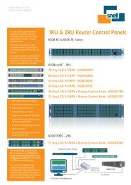
Fig 1.2.1 illustrates a number of applications in which some form of standards
conversion is employed. The classical standards converter came into being for
international interchange and converted between NTSC and PAL/SECAM.
However, practical standards converters do more than that. Many standards
converters are equipped with comprehensive signal adjustments and are sometimes
2

used to correct misaligned signals. With the same standard on input and output a
converter may act as a frame synchroniser or resolve Sc-H or colour framing
problems. As a practical matter many such converters also accept NTSC4.43 and U-
matic dub signals. There are now a number of High Definition standards and these
have led to a requirement for converters which can interface between different
HDTV standards and between HDTV and standard definition (SDTV) systems.
Program material produced in an HD format requires downconversion if it is to be
seen on conventional broadcast systems. Exchange in the opposite direction is
known as upconversion.
When television began, displays were small, not very bright and quality
expectations were rather lower. Modern CRTs can deliver much more brightness on
larger screens. Unfortunately the frequency response of the eye is extended on bright
sources, and this renders field-rate flicker visible. There is also a trend towards
larger displays, and this makes the situation worse as flicker is more noticeable in
peripheral vision than in the central area.
PAL
SECAM
NTSC
NTSC4.43
U-matic dub
50 ↔ 60
convert
PAL
SECAM
NTSC
NTSC4.43
U-matic dub
1250/50
1125/50
525/60
625/50
50 ↔ 60
convert
1250/50
1125/50
525/60
625/50
Line & field
625/50 1250/100
double
24Hz film
Rate
convert
50Hz video
60Hz video
Fig 1.2.1 a) Standards converter applications include the classical 525/625
converter
b) HDTV/SDTV conversion
c) and display related converters which double the line and field rate
Telecine is a neglected conversion area and standards conversion
can be applied from 24 Hz film to video field rates.
3

One solution to large area flicker is to use a display which is driven by a form of
standards converter which doubles the field rate. The flicker is then beyond the
response of the eye. Line doubling may be used at the same time in order to render
the line structure less visible on a large screen. Film obviously does not use interlace,
but is frame based and at 24Hz the frame rate is different to all common video
standards. Telecine machines with 50Hz output overcome the disparity of picture
rates by forcing the film to run at 25 Hz and repeating each frame twice. 60Hz
telecine machines repeat alternate frames two or three times: the well known 3:2
pulldown. The motion portrayal of these approaches is poor, but until recently, this
was the best that could be done. In fact telecine is a neglected application for
standards conversion. 3:2 pulldown cause motion artifacts in 60Hz video, but this is
made worse by conventional standards conversion to 50 Hz.
The effect was first seen when American programs which were originally edited
on film changed to editing on 60Hz video. The results after conversion to 50Hz
were extremely disappointing. Specialist standards converters were built which
could identify the third repeat field and discard it, thus returning to the original film
frame rate and simplifying the conversion to 50 Hz.
1.3 Converter block diagram
The timing of the input side of a standards converter is entirely controlled by the
input video signal. On the output side, timing is controlled by a station reference
input so that all outputs will be reference synchronous. The disparity between input
timing and reference timing is overcome using an interpolation process which
ideally computes what the video signal would have been if a camera of the output
standard and timing had been used in the first place. Such interpolation was first
performed using analogue circuitry, but was extremely difficult and expensive to
implement and prone to drift. Digital circuitry is a natural solution to such
difficulties.
The ideal is to pass the details and motion of the input image unchanged despite
the change in standard. In practice the ideal cannot be met, not because of any lack
of skill on the part of designers, but because of the fundamental nature of television
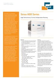
signals which will be explored in due course. Fig 1.3.1a) shows the block diagram of
an early digital standards converter. As stated earlier, the filtering process which
changes the line and field rate can only be performed on component signals, so a
suitable decoder is necessary if a composite input is to be used. The converter has
three signal paths, one for each component, and a common control system. At the
output of the converter a suitable composite encoder is also required. As the signal
to be converted passes through each stage in turn, a shortcoming in any one can
result in impaired quality.
4

High quality standards conversion implies high quality decoding and encoding. In
early converters digital circuitry was expensive, consumed a great deal of power and
was only used where essential. The decode and encode stages were analog, and
converters were placed between the coders and the digital circuitry. Fig 1.3.1b)
shows a later design of standards converter. As digital circuitry has become cheaper
and power consumption has fallen, it becomes advantageous to implement more of
the machine in the digital domain. The general layout is the same as at a) but the
converters have now moved nearer the input and output so that digital decoding
and encoding can be used. The complex processes needed in advanced decoding are
more easily implemented in the digital domain.
a)
Composite
in
Analogue
PAL/SECAM/NTSC
decoder
ADCs
Luminance
interpolator
DACs
Analogue
PAL/SECAM/NTSC
encoder
Composite
out
DEMOD
R-Y
interpolator
B-Y
interpolator
MOD
F sc
b)
Digital
Decoder
Digital
Encoder
Composite
in
ADC
Luminance
interpolator
DAC
Composite
out
DEMOD
MOD
Component
digital in
DEMUX
R-Y
interpolator
B-Y
interpolator
MUX
Component
digital out
Fig 1.3.1
Block diagram of digital standards converters. Conversion can only
take place on component signals.
a) early design using analogue encoding and decoding. Later designs
b) use digital techniques throughout.
5

A further advantage of digital circuitry is that it is more readily able to change its
mode of operation than is analogue circuitry. Such programmable logic allows, for
example, a wider range of input and output standards to be implemented. As digital
video interfaces have become more common, standards converters increasingly
included multiplexers to allow component digital inputs to be used. Component
digital outputs are also available. In converters having only analogue connections,
the internal sampling rate was arbitrary. With digital interfacing, the internal
sampling rate must now be compatible with CCIR 601. Comprehensive controls are
generally provided to allow adjustment of timing, levels and phases. In NTSC, the
use of a pedestal which lifts the voltage of black level above blanking is allowed, but
not always used, and a level control is needed to give consistent results in 50Hz
systems which do not use pedestal.
6

SECTION 2 - SOME BASIC PRINCIPLES
2.1 Sampling theory
Sampling is simply the process of representing something continuous by periodic
measurement. Whilst sampling is often considered to be synonymous with digital
systems, in fact this is not the case. Sampling is in fact an analogue process and
occurs extensively in analogue video. Sampling can take place on a time varying
signal, in which case it will have a temporal sampling rate measured in Hertz(Hz).
Alternatively sampling may take place on a parameter which varies with distance, in
which case it will have a sample spacing or spatial sampling rate measured in cycles
per picture height (c/p.h) or width. Where a two dimensional image is sampled,
samples will be taken on a sampling grid or lattice. Film cameras sample a
continuous world at the frame rate. Television cameras do so at field rate. In
addition, TV fields are vertically sampled into lines. If video is to be converted to
the digital domain the lines will be sampled a third time horizontally before
converting the analogue value of each sample to a numerical code value. Fig 2.1.1
shows the three dimensions in which sampling must be considered.
Vertical image
axis
Time axis
Horizontal image axis
Fig 2.1.1
The three dimensions concerned with standards conversion. Two of
these, vertical and horizontal, are spatial, the third is temporal.
Vertical and horizontal spatial sampling occurs in the plane of the screen, and
temporal sampling occurs at right angles (orthogonally sounds more impressive).
The diagram represents a spatio-temporal volume. Standards conversion consists of
expressing moving images sampled on one three-dimensional sampling lattice on a
different lattice. Ideally the sample values change without the moving images
7

changing. In short it is a form of sampling rate conversion in more than one
dimension. Fig 2.1.2a) shows that sampling is essentially an amplitude modulation
process. The sampling clock is a pulse train which acts like a carrier, and it is
amplitude modulated by the baseband signal. Much of the theory involved
resembles that used in AM radio. It is intuitive that if sampling is done at a high
enough rate the original signal is preserved in the samples. This is shown in Fig
2.1.2b).
a)
a)
Fig 2.1.2 Sampling is a modulation process.
a) The sampling clock is amplitude modulated by the input waveform.
b) A high sampling rate is intuitively adequate, but if the sampling rate
is too low, aliasing occurs c).
However, if the sampling rate or spacing is inadequate, there is a considerable
corruption of the signal as shown in Fig 2.1.2c). This is known as aliasing and is a
phenomenon which occurs in all sampled systems where the sampling rate is
inadequate. Aliasing can be visualised by a number of analogies. Imagine living in a
light-tight box where the door is opened briefly once every 25 hours. A completely
misleading view of the length of the day will be formed.
8

a)
0
Frequency
Fs
2Fs
b)
c)
Fs
d)
LPF response
f)
Aliasing zones
Fig 2.1.3 Sampling in the frequency domain.
a) The sampling clock spectrum.
b) The baseband signal spectrum.
c) Sidebands resulting from the amplitude modulation process of
sampling.
d) Low-pass filter returns sampled signal to continuous signal.
e) Insufficient sampling rate results in sidebands overlapping the
baseband causing aliasing.
Fig 2.1.3 shows the spectra associated with sampling. It should be borne in mind
that the horizontal axis may represent either spatial or temporal frequency. At a) the
sampling clock has a spectrum which contains endless harmonics because it is a
pulse train. At b) the spectrum of the signal to be sampled is shown. At c) the
amplitude modulation of the sampling clock by the baseband signal has resulted in
sidebands or images above and below the sampling clock frequencies. These images
can be rejected by a filter of response d) which returns the waveform to the
baseband. This is correct sampling operation. It will be seen that the limit is reached
when the baseband reaches to half the sampling rate. However, e) shows the result
if this rule is not observed. The images and the baseband overlap, and difference
frequencies or aliases are generated in the baseband.
9

To prevent aliasing, a band limiting or anti-aliasing filter must be placed before
the sampling stage in order to prevent frequencies of more than half the sampling
rate from entering. In systems which sample electrical waveforms, such a filter is
simple to include. For example all digital audio equipment uses an adequate
sampling rate and contains such a filter and aliasing is never a concern. In video
such a generalisation is untrue. CCD cameras have sensors which are split into
discrete elements and these sample the image spatially. Many cameras have an
optical anti-aliasing filter fitted above the sensor which causes a slight defocusing
effect on the image prior to spatial sampling. In interlaced CCD cameras, the output
on a given line may be a function of two lines of pixels which will have a similar
effect. Unfortunately the same cannot be said for the temporal aspects of video. The
temporal sampling rate (the field rate) is quite low for economic reasons. In fact it is
just high enough to avoid flicker at moderate brightness. As a result the bandwidth
available is quite low: half the field rate. In addition, there is no such thing as a
temporal optical anti-aliasing filter.
With a fixed camera and scene,temporal frequencies can only result from changes
in lighting, but as soon as there is relative motion, this is not the case. Brightness
variations in a detailed object are effectively scanned past a fixed point on the
camera sensor and the result is a high temporal frequency which easily exceeds half
the sampling rate. As there is no anti-aliasing filter to stop it, video signals are
riddled with temporal aliasing even on slow moving detail. However, there are other
axes passing through the spatio-temporal volume on which aliasing is greatly
reduced. When the eye tracks motion, the time axis perceived by the eye is not
parallel to the time axis of the video signal, but is on one of the axes mentioned.
More will be said about this subject when motion compensation is discussed.
Standards conversion was defined above to be a multi-dimensional case of
sampling rate conversion. Unfortunately much of the theory of sampling rate
conversion only holds if the sampled information has been correctly band limited by
an anti-aliasing filter. Standards converters are forced to use real world signals
which violate sampling theory from time to time. Transparent standards conversion
is not always possible on such signals. Standards converter design is an art form
because remarkably good results are obtained despite the odds.
10

2.2 Aperture effect
The sampling theory considered so far assumed that the sampling clock contained
pulses which were of infinitely short duration. In practice this cannot be achieved
and all real equipment must have sampling pulses which are finite. In many cases
the sampling pulse may represent a substantial part of the sampling period. The
relationship between the pulse period and the sampling period is known as the
aperture ratio. Transform theory reveals what happens if the pulse width is
increased. Fig 2.2.1 shows that the resulting spectrum is no longer uniform, but has
a sinx/x roll-off known as the aperture effect. In the case where the aperture ratio is
100%, the frequency response falls to zero at the sampling rate.
Max
0.64
Level
0 F s
Frequency
2F s
3F s
F b = F s/ 2
11
Fig 2.2.1
Aperture effect. An aperture ratio of 100% causes the frequency
response to fall to zero at the sampling rate. Reducing the aperture
ratio reduces the loss at the band edge.
This results in a loss of about 4dB at the edge of the baseband. The loss can be
reduced by reducing the aperture ratio. An understanding of the consequences of the
aperture effect is important as it will be found in a large number of processes related
to standards conversion. As it is related to sampling theory, the aperture effect can
be found in both spatial and temporal domains. In a CCD camera the sensitivity is
proportional to the aperture ratio because a reduction in the AR would require
smaller pixel area. Thus cameras have a poor spatial frequency response which
begins to roll off well before the band edge. Aperture effect means that the actual
information content of a television signal is considerably less than the standard is
capable of carrying. Fig 2.2.2a) shows the vertical spatial response of an HDTV
camera, which suffers a roll-off due to aperture effect.

The theoretical vertical bandwidth of a conventional definition system is half that
of the HDTV system. A downconverter needs a low pass filter which restricts
frequencies to those which the output standard can handle. Fig 2.2.2b) shows the
result of passing an HDTV signal into such a filter. If this is compared with the
response of a camera working at the output line standard shown at Fig 2.2.2c), it
will be seen that the result is considerably better. Thus downconverted HDTV
pictures have better resolution than pictures made entirely in the output standard.
Effectively the HDTV camera is being used as a spatially oversampling conventional
camera.
CRT displays also suffer from aperture effect because the diameter of the electron
beam is quite large compared to the line spacing. Once more a CRT cannot display
as much information as the line standard can carry. The problem can be overcome
by reversing the argument above.
a)
Vertical frequency
b)
SDTV bandwidth
c)
Fig 2.2.2
Oversampling can be used to reduce the aperture effect in
cameras.
a) the vertical aperture effect in an HDTV camera.
b) The HDTV signal is downconverted to SDTV in a digital converter
with an optimum aperture. The frequency response is much better
than the result from an SDTV camera shown at c).
An upconverter is used to convert the conventional definition signal into an
HDTV signal which is viewed on an HDTV display. The aperture effect of the
HDTV display results in a roll-off of spatial frequencies which is outside the
12

andwidth of the input signal. The HDTV display is being used as a spatially
oversampling conventional definition display. The subjective results of viewing an
oversampled display which has come from an oversampled camera are very close to
those obtained with a full HDTV system, yet the signals can be passed through
existing SDTV channels.
2.3 Interlace
Interlace was adopted in order to conserve broadcast bandwidth by sending only
half the picture lines in each field. The flicker rate is perceived to be the field rate,
but the information rate is determined by the frame rate, which is halved. Whilst the
reasons for adopting interlace were valid at the time, it has numerous drawbacks
and makes standards conversion more difficult. Fig 2.3.1a) shows a cross section
through interlaced fields. In the terminology of standards conversion it is a
vertical/temporal diagram. It will be seen that on a given row, the lines only appear
at frame rate and in any given column the lines appear at a spacing of two lines. On
stationary scenes, the fields can be superimposed to give full vertical resolution, but
once motion occurs, the vertical resolution is halved, and in practice contains
aliasing rather than useful information. The vertical/temporal spectrum of an
interlaced signal is shown in Fig 2.3.1b).
Field 2 Field 1
Vertical
distance
Time
Fig 2.3.1 a) In an interlaced system, fields contain half of the lines in a frame as
shown in this vertical/temporal diagram.
It will be seen that the energy distribution has the same pattern as in the
vertical/temporal diagram. In order to convert from one interlaced standard to
another, it is necessary to filter in two dimensions simultaneously.
13

2.4 Kell effect
In conventional tube cameras and CRTs the horizontal dimension is continuous,
whereas the vertical dimension is sampled. The aperture effect means that the
vertical resolution in real systems will be less than sampling theory permits, and to
obtain equal horizontal and vertical resolutions a greater number of lines is
necessary.
Frame period
Field period
1 cycle
per field line
1 cycle
per frame line
Temporal
frequency
Vertical spatial
frequency
Fig 2.3.1 b) The two dimensional spectrum of an interlaced system.
The magnitude of the increase is described by the so called Kell factor, although
the term factor is a misnomer since it can have a range of values depending on the
apertures in use and the methods used to measure resolution. In digital video,
sampling takes place in horizontal and vertical dimensions, and the Kell parameter
becomes unnecessary. The outputs of digital systems will, however, be displayed on
raster scan CRTs, and the Kell parameter of the display will then be effectively in
series with the other system constraints.
2.5 Quantizing
Quantizing is the process of expressing some infinitely variable quantity by
discrete or stepped values. In video the values to be quantized are infinitely variable
voltages from an analogue source. Strict quantizing is a process which operates in
the voltage domain only. For the purpose of studying the quantizing of a single
14

sample, time is assumed to stand still. This is achieved in practice by the use of a
flash converter which operates before the sampling stage. Fig 2.5.1 shows that the
process of quantizing divides the voltage range up into quantizing intervals Q, also
referred to as steps S. The term LSB (least significant bit) will also be found in place
of quantizing interval in some treatments, but this is a poor term because quantizing
works in the voltage domain. A bit is not a unit of voltage and can only have two
values. In studying quantizing, voltages within a quantizing interval will be
discussed, but there is no such thing as a fraction of a bit.
Q n+3
Voltage
axis
Q n+2
Q n+1
Q
n
Fig 2.5.1
Quantizing divides the voltage range up into equal intervals Q. The
quantized value is the number of the interval in which the input
voltage falls.
Whatever the exact voltage of the input signal, the quantizer will locate the
quantizing interval in which it lies. In what may be considered a separate step, the
quantizing interval is then allocated a code value which is typically some form of
binary number. The information sent is the number of the quantizing interval in
which the input voltage lay. Whereabouts that voltage lay within the interval is not
conveyed, and this mechanism puts a limit on the accuracy of the quantizer.
When the number of the quantizing interval is converted back to the analogue
domain, it will result in a voltage at the centre of the quantizing interval as this
minimises the magnitude of the error between input and output. The number range
is limited by the word length of the binary numbers used. In an eight-bit system,
256 different quantizing intervals exist; ten-bit systems have 1024 intervals,
although in digital video interfaces the codes at the extreme ends of the range are
reserved for synchronizing.
15

2.6 Quantizing error
It is possible to draw a transfer function for such an ideal quantizer followed by
an ideal DAC, and this is shown in Fig 2.6.1. A transfer function is simply a graph
of the output with respect to the input. In circuit theory, when the term linearity is
used, this generally means the overall straightness of the transfer function. Linearity
is a goal in video, yet it will be seen that an ideal quantizer is anything but linear.
The transfer function is somewhat like a staircase, and blanking level is half way up
a quantizing interval, or on the centre of a tread. This is the so-called mid-tread
quantizer which is universally used in digital video and audio.
Output
Input
Quantisng
error
Fig 2.6.1
Transfer function of an ideal ADC followed by an ideal DAC is a
staircase as shown here. Quantizing error is a saw tooth-like
function of input voltage.
Quantizing causes a voltage error in the video sample which is given by the
difference between the actual staircase transfer function and the ideal straight line.
This is shown in Fig 2.6.1 to be a saw-tooth like function which is periodic in Q.
The amplitude cannot exceed +/-1/2Q peak-to-peak unless the input is so large that
clipping occurs. Quantizing error can also be studied in the time domain where it is
better to avoid complicating matters with any aperture effect. For this reason it is
assumed here that output samples are of negligible duration. Then impulses from
the DAC can be compared with the original analogue waveform and the difference
will be impulses representing the quantizing error waveform. This has been done in
Fig 2.6.2.
16

The horizontal lines in the drawing are the boundaries between the quantizing
intervals, and the curve is the input waveform. The vertical bars are the quantized
samples which reach to the centre of the quantizing interval. The quantizing error
waveform shown at b) can be thought of as an unwanted signal which the
quantizing process adds to the perfect original. If a very small input signal remains
within one quantizing interval, the quantizing error becomes the signal. As the
transfer function is non-linear, ideal quantizing can cause distortion. The effect can
be visualised readily by considering a television camera viewing a uniformly painted
wall. The geometry of the lighting and the coverage of the lens means that the
brightness is not absolutely uniform, but falls slightly at the ends of the TV lines.
Input
Output
Quantisng
error
Fig 2.6.2
Quantizing error is the difference between input and output
waveforms as shown here.
After quantizing, the gently sloping waveform is replaced by one which stays at a
constant quantizing level for many sampling periods and then suddenly jumps to the
next quantizing level. The picture then consists of areas of constant brightness with
steps between, resembling nothing more than a contour map, hence the use of the
term contouring to describe the effect. As a result practical digital video equipment
deliberately uses non-ideal quantizers to achieve linearity. At high signal levels,
quantizing error is effectively noise. As the depth of modulation falls, the quantizing
error of an ideal quantizer becomes more strongly correlated with the signal and the
result is distortion, visible as contouring. If the quantizing error can be decorrelated
from the input in some way, the system can remain linear but noisy. Dither
performs the job of decorrelation by making the action of the quantizer
17

unpredictable and gives the system a noise floor like an analogue system. All
practical digital video systems use so-called nonsubtractive dither where the dither
signal is added prior to quantization and no attempt is made to remove it later.
The introduction of dither prior to a conventional quantizer inevitably causes a
slight reduction in the signal to noise ratio attainable, but this reduction is a small
price to pay for the elimination of non-linearities. The addition of dither means that
successive samples effectively find the quantizing intervals in different places on the
voltage scale. The quantizing error becomes a function of the dither, rather than a
predictable function of the input signal. The quantizing error is not eliminated, but
the subjectively unacceptable distortion is converted into a broadband noise which
is more benign to the viewer. Dither can also be understood by considering what it
does to the transfer function of the quantizer. This is normally a perfect staircase,
but in the presence of dither it is smeared horizontally until with a certain amplitude
the average transfer function becomes straight.
2.7 Digital Filters
Except for some special applications outside standards conversion, filters used in
video signals must exhibit a linear phase characteristic. This means that all
frequencies take the same time to pass through the filter. If a filter acts like a
constant delay, at the output there will be a phase shift linearly proportional to
frequency, hence the term linear phase. If such filters are not used, the effect is
obvious on the screen, as sharp edges of objects become smeared as different
frequency components of the edge appear at different times along the line. An
alternative way of defining phase linearity is to consider the impulse response rather
than the frequency response. Any filter having a symmetrical impulse response will
be phase linear. The impulse response of a filter is simply the Fourier transform of
the frequency response. If one is known, the other follows from it. Fig 2.7.1 shows
that when a symmetrical impulse response is required in a spatial system, the output
spreads equally in both directions with respect to the input impulse and in theory
extends to infinity. However, if a temporal system is considered, the output must
begin before the input has arrived, which is clearly impossible.
18

Focussed light
source
Intensity
Distance
Defocussed light
source
Intensity
a)
Distance
Intensity function spreads in both directions
Fig 2.7.1 a) When a light beam is defocused, it spreads in all directions. In a
scanned system, reproducing the effect requires an output to begin
before the input.
b) In practice the filter is arranged to cause delay as shown so that it
can be causal.
Input Impulse
Time
ÏDelay
b)
Output Impulse
Time
Symmetrical response
for phase linearity
In practice the impulse response is truncated from infinity to some practical time
span or window and the filter is arranged to have a fixed delay of half that window
so that the correct symmetrical impulse response can be obtained without
19

clairvoyant powers. Shortening the impulse from infinity gives rise to the name of
Finite Impulse Response (FIR) filter. An FIR filter can be thought of an an ideal
filter of infinite length in series with a filter which has a rectangular impulse
response equal to the size of the window. The windowing causes an aperture effect
which results in ripples in the frequency response of the filter.
Ideal filter
-infinite window
Frequency
Practical filter
-finite window
Premature roll-off
Frequency
Ripples
Fig 2.7.2
The effect of a finite window is to impair the ideal frequency
response as shown here.
Fig 2.7.2 shows the effect which is known as Gibbs’ phenomenon. Instead of
simply truncating the impulse response, a variety of window functions may be
employed which allow different trade-offs in performance. A digital filter simply has
to create the correct response to an impulse. In the digital domain, an impulse is one
sample of non-zero value in the midst of a series of zero-valued samples.
20

In
Delays
Impulse response
( sinx/ x
)
etc.
Output Impulse
etc.
Coefficients
Multiply by
coefficients
Adders
Out
Fig 2.7.3
An example of a digital low-pass filter. The windowed impulse
response is sampled to obtain the coefficients. As the input sample
shifts across the register it is multiplied by each coefficient in turn to
produce the output impulse.
Fig 2.7.3 shows an example of a low-pass filter having an ideal rectangular
frequency response. The Fourier transform of a rectangle is a sinx/x curve which is
the required impulse response. The sinx/x curve is sampled at the sampling rate in
use in order to provide a series of coefficients. The filter delay is broken down into
steps of one sample period each by using a shift register. The input impulse is shifted
through the register and at each step is multiplied by one of the coefficients. The
result is that an output impulse is created whose shape is determined by the
coefficients but whose amplitude is proportional to the amplitude of the input
impulse. The provision of an adder which has one input for every multiplier output
allows the impulse responses of a stream of input samples to be convolved into the
output waveform.
There are various ways in which such a filter can be implemented. Hardware may
be configured as shown, or in a number of alternative arrangements which give the
same results. Alternatively the filtering process may be performed algorithmically in
a processor which is programmed to multiply and accumulate. The simple filter
shown here has the same input and output sampling rate. Filters in which these rates
are different are considered in section 3.
21

2.8 Composite video
For colour television broadcast in a single channel, the PAL and NTSC systems
interleave into the spectrum of a monochrome signal a subcarrier which carries two
colour difference signals of restricted bandwidth using quadrature modulation. The
subcarrier is intended to be invisible on the screen of a monochrome television set.
A subcarrier based colour signal is generally referred to as composite video, and the
modulated subcarrier is called chroma. In NTSC, the chroma modulation process
takes the spectrum of the I and Q signals and produces upper and lower sidebands
around the frequency of subcarrier. Since both colour and luminance signals have
gaps in their spectra at multiples of line rate, it follows that the two spectra can be
made to interleave and share the same spectrum if an appropriate subcarrier
frequency is selected.
0°
180°
Ïnversion
180°
0°
Fig 2.8.1
The half cycle offset of NTSC subcarrier means that it is inverted on
alternate lines. This helps to reduce visibility on monochrome sets.
The subcarrier frequency of NTSC is an odd multiple of half line rate; 227.5
times to be precise. Fig 2.8.1 shows that this frequency means that on successive
lines the subcarrier will be phase inverted. There is thus a two-line sequence of
subcarrier, responsible for a vertical component of half line frequency.
The existence of line pairs means that two frames or four fields must elapse
before the same relationship between line pairs and frame sync. repeats. This is
responsible for a temporal frequency component of half the frame rate. These two
frequency components can be seen in the vertical/temporal spectrum of Fig 2.8.2.
22

Colour frame period
(4-field sequence)
Frame period
Field period
Luma
Two-line vertical
sequence
Temporal
frequency
Chroma
Vertical spatial
frequency
Fig 2.8.2
Vertical/temporal spectrum of NTSC shows the spectral interleave of
luminance and chroma.
When the PAL (Phase Alternating Line) system was being developed, it was
decided to achieve immunity to the received phase errors to which NTSC is
susceptible. Fig 2.8.3a) shows how this was achieved. The two colour difference
signals U and V are used to quadrature modulate a subcarrier in a similar way as for
NTSC, except that the phase of the V signal is reversed on alternate lines. The
receiver must then re-invert the V signal in sympathy. If a phase error occurs in
transmission, it will cause the phase of V to alternately lead and lag, as shown in Fig
2.8.3b). If the colour difference signals are averaged over two lines, the phase error
is eliminated and then replaced with a small saturation error which is subjectively
much less visible. This does, however, have a fundamental effect on the spectrum.
23

Line n received with
phase error ‘e’
Line n+1 received with
phase error ‘e’
Average of line n and n+1 removes
error ‘e’, restoring transmitted phase
Fig 2.8.3
In PAL the V signal is inverted on alternate lines. On reception, this
turns a static phase error into an alternating amplitude error in U and
V which can be averaged out.
The vertical/temporal spectrum of the U signal is identical to that of luminance.
However, the inversion of V on alternate lines causes a two line sequence which is
responsible for a vertical frequency component of half line rate. As the two line
sequence does not divide into 625 lines, two frames elapse before the same
relationship between V-switch and the line number repeats. This is responsible for a
half frame rate temporal frequency component.
24

Colour frame period
(eight-field sequence)
U
Y
V
Four-line
vertical
sequence
Fig 2.8.4
The vertical/temporal spectrum of PAL is more complex than that of
NTSC because of V-switch.
Fig 2.8.4 shows the resultant vertical/temporal spectrum of PAL. Spectral
interleaving with a half cycle offset of subcarrier frequency as in NTSC will not
work and a subcarrier frequency with a quarter cycle per line offset is needed
because the V component has shifted diagonally so that its spectral entries lie half
way between the U component entries. Note that there is an area of the spectrum
which appears not to contain signal energy in PAL. This is known as the Fukinuki
hole. The quarter cycle offset is thus a fundamental consequence of elimination of
phase errors and means that there are now line quartets instead of line pairs. This
results in a vertical frequency component of one quarter of line rate which can be
seen in the figure.
SECAM (Sequential à memoire) is a composite system which sends the colour
difference signals sequentially on alternate lines by frequency modulating the
subcarrier, which will have one of two different centre frequencies. The alternating
subcarrier frequencies result in a vertical component of half line rate and a four field
sequence. Although it resists multipath transmission well, it cannot be processed for
production purposes because of the FM chroma.
25

2.9 Composite decoding
The reason for the difficulty in properly decoding composite video is the
complexity of the spectrum, particularly in the case of PAL. Chroma and luminance
information are spectrally interleaved in two dimensions and must be precisely
separated before the chroma can be demodulated. One way in which the two signals
can be separated is to use the repetitive response of a comb filter.
Input
1 line
Delays
1 line
Luminance
Chrominance
Fig 2.9.1
A simple line comb filter for Y/C separation needs considerable
modification for practical use. See text for details.
Fig 2.9.1 shows a simple comb filter consisting of two RAM delays and a three
input adder. The frequency response is a cosinusoid with the peaks spaced at the
reciprocal of the delay. For Y/C separation the delay needs to be one line period
long. Although the spectral response is reasonably good, offering minimal crosscolour
and cross-luminance, there are some shortcomings.
Firstly, the summing of the three filter taps which rejects chroma also results in
the adding together of luminance at the same points in three different TV lines. In
other words, the comb filter configuration which gives the correct frequency
response for chroma separation inadvertently results in a transversal low-pass
filtering action on luminance signals in the vertical axis of the screen. Vertical
resolution will be reduced. Secondly the comb filter is working not with a static
subcarrier, but with dynamically changing chroma. Optimal chroma rejection only
takes place when chroma phase is the same in the three successive lines forming the
filter aperture. This will not be the case when there are vertical colour changes in
the picture. Vertical colour changes cause the filter to suffer what is known as comb
mesh failure. Full chroma rejection is not achieved and the luminance signal for the
duration of the failure will contain residual chroma which manifests itself as a series
of white dots, known as “hanging dots”, at horizontal boundaries between colours.
Comb mesh failure can be detected by analysing the chroma signals at the ends of
the comb, and if chroma will not be cancelled, the high frequency luminance is not
added back to the main channel, and a low pass response results. Since the chroma
signal is symmetrically disposed about the subcarrier frequency, there is no chroma
26

to remove from the lower luminance frequencies, and thus there is no need to
continue the comb filter response in that region.
The simple filter of Fig 2.9.1 has a comb response from DC upwards. The
vertical resolution loss of such a filter can be largely restored by running the comb
filter only in a passband centred around subcarrier. Within the passband, combing
is used to remove luminance from the chroma. This chroma is then subtracted from
the composite input signal to leave luminance. Below the passband the entire input
spectrum is passed as luminance and the vertical resolution loss is restored. The line
comb gives quite good results in NTSC, as horizontal and vertical resolution are
good, but the loss of vertical resolution at high frequency means that diagonal
resolution is poor. A line comb filter is at a disadvantage in PAL because of the
spreading between U and V components. What is needed is a comb filter having
delays of two lines, but this will have an even more severe effect on diagonal
frequencies, so PAL comb filters are often found with only single line delays, a
choice influenced by commonality with an NTSC product. Although the three
dimensional spectrum of PAL is complicated, it is possible to combine elements of
both vertical and temporal types of filter to obtain a spatio-temporal response
which is closely matched to the characteristics of PAL.
27

Vertical spatial
frequency
Temporal
frequency
Fig 2.9.2
A vertical temporal filter with the response shown has better
performance on PAL signals and does not need to be adaptive.
Fig 2.9.2 shows the vertical/temporal response of such a filter. By following the
diagonal structure of the PAL spectrum, the passbands of the signal components are
much wider. The vertical frequency response is around three times better than that
of a two-line delay vertical comb and the temporal frequency response exceeds that
of the field delay based temporal comb by the same factor. Whilst complex, this
approach has the advantage that a fixed response can be used and adaptive circuitry
is dispensed with. The absence of adaptation results in better handling of difficult
material.
28

SECTION 3 - STANDARDS CONVERSION
3.1 Interpolation
Practical standards conversion takes place in three dimensions as shown above.
For clarity, it is proposed here to begin with a single dimensional system in order to
show the principles clearly. Fig 3.1.1 shows that standards conversion requires a
form of sampling rate conversion where the same waveform must be expressed by
samples at different places. One way of converting is to return to the analogue
domain and simply to sample the analogue signal on a new sampling lattice. There
are many reasons for not doing so, particularly that two additional conversion and
filtering processes add unnecessary quality impairment. In fact a return to the
analogue domain is quite unnecessary as digital interpolation can be used.
Interpolation is the process of computing the value of a sample or samples which lie
off the sampling matrix of the source signal. It is not immediately obvious how
interpolation works as the input samples appear to be points with nothing between
them.
Original analogue
waveform
Input
samples
Output
samples
Fig 3.1.1
Sampling rate conversion consists of expressing the original
waveform with samples in different places.
One way of considering interpolation is to treat it as a digital simulation of a
digital to analogue conversion. According to sampling theory, all sampled systems
have finite bandwidth. An individual digital sample value is obtained by sampling
the instantaneous voltage of the original analogue waveform, and because it has
zero duration, it must contain an infinite spectrum. However, such a sample can
never be seen in that form because the spectrum of the impulse is limited to half of
the sampling rate in a reconstruction or anti-image filter. The impulse response of
an ideal filter converts each infinitely short digital sample into a sinx/x pulse whose
central peak width is determined by the response of the reconstruction filter, and
whose amplitude is proportional to the sample value. This implies that, in reality,
one sample value has meaning over a considerable time span, rather than just at the
sample instant.
29

A single pixel has meaning over the two dimensions of a frame and along the
time axis. If this were not true, it would be impossible to build an interpolator. If
the cut-off frequency of the filter is one-half of the sampling rate, the impulse
response passes through zero at the sites of all other samples.
Sample
Analogue output
Sinx/ x
impulses
due to sample
etc.
etc.
Fig 3.1.2
In a reconstruction filter, the impulse response is such that it passes
through zero at the sites of adjacent samples. Thus the output
waveform joins up the tops of the samples as required.
It can be seen from Fig 3.1.2 that at the output of such a filter, the voltage at the
centre of a sample is due to that sample alone, since the value of all other samples is
zero at that instant. In other words the continuous time output waveform must join
up the tops of the input samples. In between the sample instants, the output of the
filter is the sum of the contributions from many impulses, and the waveform
smoothly joins the tops of the samples. If the waveform domain is being considered,
the anti-image filter of the frequency domain can equally well be called the
reconstruction filter. It is a consequence of the band-limiting of the original antialiasing
filter that the filtered analogue waveform could only travel between the
sample points in one way.
30

a) Input
spectrum
b) Output
spectrum
Halved
sampling rate
Aliasing
Fig 3.1.3 a) Is the spectrum of a sampled system. Reducing the sampling rate
alone causes aliasing b) as the sidebands are unchanged in width.
As the reconstruction filter has the same frequency response, the reconstructed
output waveform must be identical to the original band-limited waveform prior to
sampling. Interpolation may be used to increase or decrease the sampling rate.
Interchange between 525 and 625 line standards will require one or the other
depending on the direction, as will HDTV and SDTV interchange. Fig 3.1.3a) shows
the spectrum of a typical sampled system where the sampling rate is a little more
than twice the analogue bandwidth. Attempts to halve the sampling rate for
downconversion by simply omitting alternate samples, a process known as
decimation, will result in aliasing, as shown in b). It is intuitive that omitting every
other sample is the same as if the original sampling rate was halved. In any sampling
rate conversion system, in order to prevent aliasing, it is necessary to incorporate
low-pass filtering into the system where the cut-off frequency reflects the lower of
the two sampling rates concerned.
An FIR type low-pass filter, as described in section 2, could be installed
immediately prior to the interpolator, but this would be wasteful, as it has been seen
above that interpolation itself requires such a filter. It is much more effective to
combine the anti-aliasing function and the interpolation function in the same filter.
31

3.2 Line doubling
Input
samples
Output
samples
Fig 3.2.1
In line doubling, half of the output samples are identical to the input
samples and only the intermediate values need to be computed.
The simplest form of interpolator is one in which the sampling rate is exactly
doubled. Such an interpolator may form the basis of a line-doubling CRT display.
Fig 3.2.1 shows that half of the output samples are identical to the input, and new
samples need to be computed half way between them. The ideal impulse response
required will be a sinx/x curve which passes through zero at all adjacent input
samples. Fig 3.2.2 shows that this impulse response can be re-sampled at half the
usual sample spacing in order to compute coefficients which express the same
impulse at half the previous sample spacing. In other words, if the height of the
impulse is known, its value half a sample away can be computed. If a single input
sample is multiplied by each of these coefficients in turn, the impulse response of
that sample at the new sampling rate will be obtained.
32

Position of adjacent input samples
Analogue waveform
resulting from low-pass
filtering of input samples
0.127 -0.21 0.64 0.64 -0.21 0.127
Coefficients used in Fig 3.2.3
Fig 3.2.2
The impulse response of the reconstruction filter can be re-sampled
at a higher sampling rate to obtain coefficients between existing
samples.
Note that every other coefficient is zero, which confirms that no computation is
necessary on the existing samples; they are just transferred to the output. The
intermediate sample is computed by adding together the impulse responses of every
input sample in the window. Fig 3.2.3 shows how this mechanism operates.
33

Input samples
A B C D
Sample value
A
-0.21 X A
Contribution from
sample A
Sample value
B
0.64 X B
Contribution from
sample B
0.64 X C
Contribution from
sample C
C
Sample value
D
Sample value
-0.21 X D
Contribution from
sample D
Interpolated sample value
= -0.21A +0.64B +0.64C -0.21D
Fig 3.2.3
A line doubling interpolator which computes the contributions of
nearby samples to a point half way between an existing pair of
samples using the coefficients of Fig 3.2.2.
34

3.3 Fractional ratio interpolation
In the vertical axis of a 525/625 converter, there is a periodicity in the
relationship between the two line structures which means that an output line occurs
in one of 21 different places between input lines. This allows the use of an
interpolator which is similar to the rate doubler above, but which is capable of
computing the value of impulse responses at more places between input samples. As
a practical matter it is possible to have a system clock which runs at a common
multiple of the two rates. One way of considering the operation of a fractional ratio
interpolator is that it may consist of two integer ratio converters in series. This is
shown in Fig 3.3.1a). Clearly this is inefficient as many of the values computed in
the first stage are discarded by the second. Once more it is more efficient to combine
the two processes into a single filter as shown at b). Here only wanted output values
are computed. It will be evident that fixed coefficients are not suitable. The location
or phase of each output sample varies and Fig 3.3.1c) shows that the filter
coefficients must come from a ROM which can be addressed by the required phase.
a)
4 X
increase
3 X
reduce
Fig 3.3.1 a) A fractional ratio converter can be thought of as two integer ratio
converters in series.
b) It is far more efficient to combine the two. Each sample now requires
coefficients of a different phase (overleaf).
c) A ROM is required as shown which can be addressed by the phase
to produce the correct coefficients (overleaf).
35

a)
Data in
Phase
select
b)
FILTER
ROM
Data out
Coefficients
3.4 Variable interpolation
In converters which need to change the aspect ratio, and in motion compensated
converters, it becomes necessary to compute sample values which have an arbitrary
relationship to the input sample lattice. Thus in theory an infinite number of filter
phases and coefficients will be required. This is not possible in practice, and the
solution is to have a large but finite number of phases available.
The position of the required sample is used to select the nearest available
interpolation phase. The ideal continuous temporal or spatial axis of the
interpolator is in practice quantized by the phase spacing, and a sample value
needed at a particular point will be replaced by a value for the nearest available
filter phase. The number of phases in the filter therefore determines the accuracy of
the interpolation. The effects of calculating a value for the wrong point are identical
to those of sampling with clock jitter, in that an error occurs proportional to the
slope of the signal. The result is program-modulated noise. The higher the noise
specification, the greater the desired time accuracy and the greater the number of
phases required. The number of phases is equal to the number of sets of coefficients
available, and should not be confused with the number of points in the filter, which
is equal to the number of coefficients in a set (and the number of multiplications
needed to calculate one output value).
36

3.5 Interpolation in several dimensions
In a conventional 525/625 converter, the active line period of both standards is
so similar that it can be considered identical. In this case no horizontal manipulation
is required at all and the converter becomes a two dimensional vertical temporal
filter. In HDTV to SDTV converters the horizontal axis will also require a
conversion process. In order to design a suitable two-dimensional filter it is
necessary to consider the spectrum of the input signal. The use of interlace has a
profound effect on the vertical/temporal spectrum shown in Fig 3.5.1 which shows
values for 625/50 scanning.
Vertical
frequency c/p.h.
625
312.5
0 25 50
Temporal
frequency Hz
Fig 3.5.1
The vertical/temporal spectrum of luminance in an interlaced system
has a quincunx pattern.
The horizontal component of the star shaped spectra is due to image movement
where the higher the speed and the more detail present, the higher the temporal
frequencies will be. The vertical component of the stars is due to vertical detail in
the image. Interlace means that the same picture line is scanned once per frame,
hence the images repeating on the horizontal axis at multiples of 25 Hz. Each field
is scanned by 312 1 ¼2 lines, hence the vertical images repeating at multiples of that
rate. The result is a two-dimensional spectrum having what is known as a quincunx
pattern (resembling the five of dice). In order to perform interpolation or
reconstruction on such a spectrum, it is necessary to incorporate a low-pass filter as
has been seen above.
37

Vertical
frequency
Stop
band
Temporal
frequency
Triangular
passband
Fig 3.5.2
In order to return to the baseband in an interlaced system a twodimensional
filter with a triangular response is required.
The interpolation process must incorporate a two dimensional filter having a
triangular passband shown in Fig 3.5.2 which passes the baseband spectrum and
rejects the images. The interpolator works in two dimensions to express the input
data at a different line and field rate. In some cases it is possible to construct a two
dimensional interpolator using two one-dimensional filters in series.
Fig 3.5.3 shows how this can be done. Unfortunately the result must always be a
rectangular two-dimensional spectrum and it should be clear that this is of no use
whatsoever for filtering an interlaced signal. Fig 3.5.4a) shows the structure of a
four field by four line standards converter. Field and line delays are combined so
that simultaneous access to sixteen pixels is available.
38

Vertical
frequency
After
vertical
low-pass
filter
Stop band
Passband
Temporal
frequency
Vertical
frequency
After
vertical &
temporal
low-pass
filter
Stop band
(vertical)
Rectangular
passband
Stop band
(temporal)
Temporal
frequency
Fig 3.5.3
If two one-dimensional filters are used, the result can only be a
rectangular passband which is of no use in an interlaced system.
Field delay
Pixel delay
In
Coefficients
Out
Fig 3.5.4 a) A four line by four field two dimensional filter. The location of input
samples in the vertical/temporal space is shown in b) overleaf.
39

Vertical
axis
Time axis
Fig 3.5.4 b) The location of input samples in the vertical/temporal space.
Fig 3.5.4b) show the sixteen points are distributed in the vertical/temporal space.
Although four lines in each field contribute, the effective vertical aperture is eight
picture lines because of interlace. The ideal frequency response of Fig 3.5.3 cannot
be achieved by the practical filter of Fig 3.5.4. The reason is that an ideal filter
requires an infinite window, whereas all practical filters must use finite windows. In
a vertical/temporal filter, the vertical window size is determined by the number of
lines which contribute to a given output sample and the temporal window size is
determined by the number of fields which contribute. Clearly the provision of more
fields raises the amount of RAM required in proportion and this carries a cost
penalty. As was shown in section 2.8, shortening, or truncating, the theoretical
impulse response impairs the frequency response. The response begins to fall before
the band edge, and there are ripples in the stop band. In practice if one is improved,
the other deteriorates. A compromise must be found between the two.
The ripples in the stop band cause the greatest concern because they pass image
frequencies which should be suppressed. After the sampling rate conversion these
frequencies alias to beat frequencies.
40

Input
spectrum
a)
After ideal
filter
After non-ideal
filter
b)
After
resampling
Aliased components
inside baseband
Fig 3.5.5 a) With an ideal filter, the images of the input spectrum are rejected
and the resampling process produces a clean set of images at the
new sampling rate.
b) With a non-ideal filter, some of the input images are unsuppressed
and cause aliasing when resampled at the output rate.
Fig 3.5.5 shows how this happens in one dimension. The ideal situation is shown
at a), in which a 50Hz sampled signal is adequately filtered to the baseband and
resampled at 60Hz. The resultant spectrum is free of aliasing. However, if the filter
is imperfect, as shown at b), some energy at 50Hz remains, and when sampled at
60Hz it will alias to 10Hz.
41

Vertical
frequency
Unsuppressed
= Modulation of
moving edges
Unsuppressed
=Vertical aliasing
Unsuppressed
=5Hz flicker
Roll-off here
= Loss of vertical
detail
Stop Band
Base Band
Roll-off here
= Motion blur
Unsuppressed
=motion judder
Temporal
frequency
Fig 3.5.6
Potential problems due to non-ideal filtering are catalogued here.
Fig 3.5.6 catalogues the problems which may occur in a two dimensional
50/60Hz filter. Premature rolling off in the passband will cause wanted frequencies
to be lost. In the vertical axis this causes loss of vertical resolution; in the temporal
axis this results in motion blur. Stop band ripples allow alias frequencies into the
passband. In the vertical axis, the spatial beat frequencies will be given by the
difference between the number of lines in the frames, i.e. 625 - 525 = 100 cycles per
picture height, and by the difference between the number of lines in the fields, i.e.
50 cycles per picture height. On the temporal axis, the beat frequencies will be given
by the differences between frame and field rates, i.e. 5 and 10 Hz.
3.6 Aperture synthesis
It is the frequency response of a two dimensional filter which is of most interest
because this determines how much impairment will be caused by unsuppressed
aliases. However, in order to implement the filter, it must be supplied with
coefficients which result from sampling the impulse response. The impulse response
and the frequency response are connected by the Fourier transform. The goal is to
design an impulse response having the best compromise between roll-off and ripple.
Aperture synthesis is a technique which makes this design process significantly
easier. Realisable filters work with a finite window, and in a sampled system there
are a finite number of samples within that window.
42

Sampling period
Sampling
frequency
a)
DFT
b)
0
Frequency
Time
d)
FT
c)
e)
Fig 3.6.1 a) The windowed impulse response of a filter.
b) The Discrete Fourier Transform of the impulse contains as many
frequencies as the window has points.
c) Each discrete frequency in the DFT represents a sinx/x spectrum in
a continuous transform.
d) The sinx/x pulse is the transform of the rectangular window.
e) The continuous spectrum is obtained by adding the sinx/x curves of
each of the discrete spectral lines. The origin of stop-band ripple
should be clear.
The values of the samples in the window can describe an impulse response as
shown in Fig 3.6.1a). Fourier analysis tells us that the spectrum of discrete signals
must also be discrete, and the number of different frequencies in the spectrum is
equal to the number of samples in the window. The spectrum of a) is shown in b).
As a consequence, the frequency response of the filter can be specified in a finite
number of evenly spaced places. In a two dimensional filter these places will form a
rectangular grid. In order to return to the continuous time domain from discrete
samples, each sample is replaced by a sinx/x impulse. The same principle holds in
the discrete frequency domain.
43

a)
Drama
aperture
+525
c/ph
Vertical
frequency
+525
c/ph
Vertical
frequency
-525
c/ph
-60Hz
Temporal
frequency
+60Hz
-525
c/ph
-60Hz
Temporal frequency
+60Hz
b)
Sports
aperture
+525
c/ph
Vertical
frequency
+525
c/ph
Vertical
frequency
-525
c/ph
-60Hz
Temporal
frequency
+60Hz
-525
c/ph
-60Hz
Temporal frequency
+60Hz
Fig 3.6.2 The responses of the filter in the ACE converter.
a) The response optimised for drama,
b) The response optimised for pans to reduce judder.
In order to return to a continuous spectrum, each spectral line is replaced by a
sinx/x spectrum c) which is in fact the transform of the rectangular windowed). The
sinx/x spectra are added to give the continuous spectrum e). It will be seen from e)
that even though the frequency response is specified at zero at the discrete points,
the sinx/x spectral components cause it to be non-zero between those points. This is
the cause of stop band ripple. The art of filter design is to juggle the passband
spectrum so that the tails of the sinx/x impulses cancel one another out rather than
reinforcing. As the effects of beat frequencies are subjectively very irritating, it is
better to eliminate them at the expense of some premature roll-off of the passband.
Today software packages are available which allow the optimising process to be
automated. Fig 3.6.2 shows the responses of the filter used in the ACE standards
converter. Clearly the response must be different depending on the direction of
conversion as the position of input frequencies needing most suppression depends
on the input spectrum. The ideal triangular response worked well on material such
as studio drama, but was found to cause excessive judder on pans. As a result an
alternative diamond shaped response was made available which reduced judder at
the cost of increased motion blur.
44

The Fourier transform of the frequency response yields the impulse response, and
this must then be sampled in two dimensions to obtain coefficients. The impulse
must be displaced by all of the necessary interpolation phases in two dimensions,
and sampled at each one into a coefficient set. As the impulse is symmetrical in two
axes, it is only necessary to store one quarter of it in ROM, the remaining three
quarters can be obtained by mirroring the vertical and/or horizontal ROM
addresses.
A vertical aperture of eight points (four per field) is sufficient for adequate
suppression of vertical artifacts, and a temporal aperture of four fields is wide
enough to remove temporal artifacts. Four field standards converters are too
expensive for some applications, and cost effective machines having two field
apertures are available. With such a short temporal aperture, it is not possible to
reach an acceptable compromise between roll-off and ripple.
Eliminating 5 Hz beating is very difficult because positioning a response null to
eliminate it results in passing the frequencies responsible for judder and vice-versa.
It is possible to increase the temporal aperture to six fields, and in theory this
produces a sharper cut-off and better suppression. However, on real input signals
the improvement will not be realised because of temporal aliasing actually in the
input signal. Another consequence of increasing the temporal aperture is that
motion portrayal is compromised.
45

3.7 Motion compensated standards conversion
Fig 3.7.1a) shows that if an object is moving, it will be in a different place in
successive fields. Interpolating between several fields, in this case four, results in
multiple images of the object. The position of the dominant image will not move
smoothly; an effect which is perceived as judder. If, however the camera is panning
the moving object, it will be in much the same place in successive fields and Fig
3.7.1b) shows that it will be the background which judders. Motion compensation
is designed to overcome this judder by taking account of the human visual
mechanism.
In the interests of
clarity, judder is only
shown at the outside
edges of the objects,
instead of all vertical
edges.
a) Fixed camera b) Panning camera
Fig 3.7.1a) Conventional four field converter with moving object produces
multiple images.
b) If the camera is panned on the moving object, the judder moves to
the background.
The eye also has a temporal response taking the form of a lag known as
persistence of vision. The effect of the lag is that resolution is lost in areas where the
image is moving rapidly over the retina; a phenomenon known as motion blur. Thus
a fixed eye has poor resolution of moving objects.
46

Fixed Eye
Moving
Object
Brightness
Time
Fig 1.1.2a Temporal Frequency = High
Tracking Eye
Moving
Object
Brightness
Moving Field
of View
Time
Fig 1.1.2b Temporal Frequency = Zero
Fig 3.7.2a) A detailed object moves past a fixed eye, causing temporal
frequencies beyond the response of the eye. This is the cause of
motion blur.
b) The eye tracks the motion and the temporal frequency becomes
zero. Motion blur cannot then occur.
In Fig 3.7.2a) a detailed object moves past a fixed eye. It does not have to move
very fast before the temporal frequency at a fixed point on the retina rises beyond
the temporal response of the eye.
Fortunately the eye can move to follow objects of interest. Fig 3.7.2b) shows the
difference this makes. The eye is following the moving object and as a result the
temporal frequency at a fixed point on the retina is DC; the full resolution is then
available because the image is stationary with respect to the eye. In real life we can
see moving objects in some detail unless they move faster than the eye can follow.
Television viewing differs from the processes of Fig 3.7.2 in that the information is
sampled. According to sampling theory, a sampling system cannot properly convey
frequencies beyond half the sampling rate. If the sampling rate is considered to be
the field rate, then no temporal frequency of more than 25 or 30 Hz can be handled.
When there is relative movement between camera and scene, detailed areas develop
high temporal frequencies, just as was shown in Fig 3.7.2 for the eye.
47

This is because relative motion results in a given point on the camera sensor
effectively scanning across the scene. The temporal frequencies generated are beyond
the limit set by sampling theory, and aliasing takes place. However, when the
resultant pictures are viewed by a human eye, this aliasing is not perceived because,
once more, the eye attempts to follow the motion of the scene.
Temporal Frequency = High
Tracking eye
Fixed
Display
Fixed Camera
Sensor
Moving
Object
Temporal
Frequency = Zero
Moving Field of View
Fig 3.7.3
An object moves past a camera, and is tracked on a monitor by the
eye. The high temporal frequencies cause aliasing in the TV signal,
but these are not perceived by the tracking eye as this reduces the
temporal frequency to zero. Compare with Fig 3.7.2.
Fig 3.7.3 shows what happens when the eye follows correctly. Effectively the
original scene and the retina are stationary with respect to one another, but the
camera sensor and display are both moving through the field of view. As a result the
temporal frequency at the eye due to the object being followed is brought to zero
and no aliasing is perceived by the viewer due to the field rate sampling.
Unfortunately, when the video signal passes through a conventional standards
converter, the aliasing on the time axis means that the input signal has not been
properly band-limited and interpolation theory breaks down. The converter cannot
tell the aliasing from genuine signals and resamples both at the new field rate. The
resulting beat frequencies cause visible judder. Motion compensation is a way of
modifying the action of a standards converter so that it follows moving objects to
eliminate judder in the same way that the eye does.
48

The basic principle of motion compensation is quite simple. In the case of a
moving object, it appears in different places in successive source fields. Motion
compensation computes where the object will be in an intermediate target field and
then shifts the object to that position in each of the source fields.
a) Input fields b) Shifted input fields
Fig 3.7.4 a) Successive fields with moving object.
b) Motion compensation shifts the fields to align position of the moving
object.
Fig 3.7.4a) shows the original fields, and Fig 3.7.4b) shows the result after
shifting. This explanation is only suitable for illustrating the processing of a single
motion such as a pan. An alternative way of looking at motion compensation is to
consider what happens in the spatio-temporal volume. A conventional standards
converter interpolates only along the time axis, whereas a motion compensated
standards converter can swivel its interpolation axis off the time axis.
49

a) Input fields
Interpolation
axis
Interpolation
axis
Time
axis
Interpolation
axis
Judder free
output field
b) Interpolation axis at
an angle to time axis
for moving objects
Fig 3.7.5 a) Input fields with moving objects.
b) Moving the interpolation axes to make them parallel to the trajectory
of each object.
Fig 3.7.5a) shows the input fields in which three objects are moving in a different
way. At b) it will be seen that the interpolation axis is aligned with the trajectory of
each moving object in turn. This has a dramatic effect. Each object is no longer
moving with respect to its own interpolation axis, and so on that axis it no longer
generates temporal frequencies due to motion and temporal aliasing cannot occur.
Interpolation along the correct axes will then result in a sequence of output fields in
which motion is properly portrayed. The process requires a standards converter
which contains filters which are modified to allow the interpolation axis to move
dynamically within each output field. The signals which move the interpolation axis
are known as motion vectors. It is the job of the motion estimation system to
provide these motion vectors. The overall performance of the converter is
determined primarily by the accuracy of the motion vectors. An incorrect vector will
result in unrelated pixels from several fields being superimposed and the result is
unsatisfactory.
50

Motion Estimator
(Measures motion)
Motion
values
Vector Assignment
(Attributes motion
to pixels)
Video
input
Motion
vectors
Motion
Compensated
Standards
Converter
Converted
video out
Fig 3.7.6
The essential stages of a motion compensated standards converter.
Fig 3.7.6 shows the sequence of events in a motion compensated standards
converter. The motion estimator measures movements between successive fields.
These motions must then be attributed to objects by creating boundaries around sets
of pixels having the same motion. The result of this process is a set of motion
vectors, hence the term vector assignment. The motion vectors are then input to a
specially designed standards converter in order to deflect the inter-field interpolation
axis. Note that motion estimation and motion compensation are two different
processes. There are several different methods of motion estimation and these are
treated in detail in “The Engineer’s Guide to Motion Compensation.”
51

SECTION 4 - APPLICATIONS
4.1 Up and down converters
Conversion between HDTV and SDTV requires some additional processes.
HDTV formats have an aspect ratio of 16:9 whereas SDTV uses 4:3.
Downconversion offers various ways of handling the mismatch. The picture may be
displayed full height with the edges cropped, or full width with black bars above
and below. It is also possible to apply a variable degree of anamorphic compression.
These processes involve the horizontal dimension which is not affected by 525/625
conversion.
These converters are truly three dimensional, because in addition to converting
the number of lines in the picture and the field rate, it is necessary to filter the
horizontal axis to reduce the input bandwidth to that allowed in the output
standard and to change the aspect ratio. The horizontal axis is not involved with
interlace and so the horizontal filtering may be performed prior to the vertical
temporal filtering or simultaneously without any performance penalty. In display
line doublers similar processes are required.
4.2 Field rate doubling
Field rate doublers are designed to eliminate flicker on bright, large screen
displays by raising the field rate. In some respects the field rate change is easier than
in a 50/60Hz converter because the output field rate can be twice the input rate and
synchronous with it. Then the output fields have a single constant temporal
relationship with the input fields which reduces the number of coefficients required.
However, with a large display the loss of resolution due to conventional conversion
may not be acceptable and motion compensation will be necessary.
4.3 DEFT
In telecine transfer the 24 Hz frame rate of film is incompatible with 50 or 60Hz
video. Traditionally some liberties are taken because there was until recently no
alternative. In 50Hz telecine the film is driven at 25 fps, not 24, so that each frame
results in two fields. In 60Hz telecine the film runs at 24 fps, but odd frames result
in two fields, even frames result in three fields; the well known 3:2 pulldown. On
average there are two and a half fields per film frame giving a field rate of 60 Hz.
The field repetition of telecine causes motion judder. The motion portrayal of
telecine is shown in Fig 4.3.1.
52

Input film frames at 24Hz
Optic flow of
film (no judder)
Judder due to
double and triple
image repeats
Fig 6a Origin of
judder for
60Hz 3:2
pulldown
telecine
2 3 60Hz output fields 2
Input film frames at 25Hz
Optic flow of
film (no judder)
Judder due to
image repeats
Fig 6b Origin of
judder for
50Hz
telecine
2 2 50Hz output fields 2
Fig 4.3.1
There is, however a worst case effect which is obtained when 60Hz telecine
material is standards converted to 50Hz video. The 3:2 pulldown judder inherent in
the 60Hz video is compounded by the judder resulting from 60/50 conversion and
the result is highly unsatisfactory. Some standards converter are adaptive, and select
different filter responses according to motion in the input. Such an adaptation
system is unable to cope with the 3:2 pulldown where there are two identical fields,
then a change followed by three identical fields. The solution is to design a
standards converter specially to deal with conversion of 60Hz video from telecine.
The converter has an input buffer which can hold several input fields and circuitry
which compares successive fields.
53

It is possible to identify the 3:2 field sequence in the input signal. The third
repeated field is discarded so that the remaining input consists of exactly two fields
for each film frame. The effective field rate is now 48 Hz, but as pairs of input fields
have come from the same film frame, they can be de-interlaced to recreate the
frames at 24 Hz. This forms the input to a standards conversion process which
outputs 50Hz interlaced video. Whilst the principle appears reasonably simple, there
is some additional complexity because video edits take place without regard to the
3:2 sequence on the tape. The converter must be able to reliably deduce what has
happened on edited material.
Field
repeats
60Hz field
30Hz frame
3
2
TV
frame
same different different same same same different
Fig 4.3.2
same different same same same different different
EDIT
breaks
3:2
sequence
In 3:2 pulldown video, there are two types of frame. One type
contains two fields from the same film frame. The other contains
fields from different frames. A video edit can break the 3:2
sequence and produce a tape with only a single field representing a
film frame.
Fig 4.3.2 shows that there are two types of input frame; one type contains fields
from the same film frame, the other contains fields from different frames. After
editing it is possible to have a film frame which is represented by a single field. In
order to follow what is happening in the input a large number of fields of storage
are required and this makes the converters expensive.
54

Glossary
Artifact
Baseband
Image
Contouring
Decimation
Dither
Hanging dots
Judder
Lag
Lattice
Linear phase
Oversampling
Sideband
Standard
a visible defect in a television picture due to a shortcoming in
some process.
signal prior to any modulation process.
see sideband.
an effect due to quantizing a luminance signal.
process of discarding excess samples to reduce sampling rate.
noise added prior to an ADC to linearise low level signals.
artifact caused by residual chroma in luminance.
artifact in which motion is portrayed in an irregular way.
term given to a low pass filtering effect in the time domain.
a grid in two or three dimensions which determines where
samples are taken.
all frequencies suffer the same delay, and impulse response is
symmetrical in a linear phase system.
using a sampling rate in excess of that required by sampling
theory.
a difference frequency resulting from the multiplicative nature
of modulation see also image.
video waveform whose parameters are approved by a
regulatory body.
55

Published by Snell & Wilcox Ltd.
Durford Mill
Petersfield
Hampshire
GU13 5AZ
Tel: +44 (0) 703 821188
Fax: +44 (0) 703 821199
Copyright © Snell & Wilcox 1994
Text and diagrams from this publication may be reproduced providing acknowledgement is
given to Snell & Wilcox.
UK £7.50
US $12.00
Engineering with Vision
56

Original analogue
waveform
Input
samples
Output
samples
3
2
3 fields
60Hz Field
2 fd
30Hz
3 fields
2 fd
3 fields
TV
frame
same different different same same same diff..
Single field at edit
3
2
3 fields
2 fd
2 fd
3 fields
2 fd
same different same same same different
EDIT
breaks
3:2
sequence
57