[Luyben] Process Mod.. - Student subdomain for University of Bath

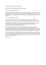
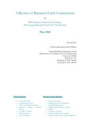
586 MULTIVARIABLE PROCESSES
‘)
log w
FIGURE 16.9
SISO closcdloop plots.
If we plotted just the denominator of the right-hand side of Eq. 16.42, the curve
would be the reciprocal of the closedloop servo transfer function and would look
something like that shown in Fig. 16.9b. The lower the dip in the curve, the lower
the damping coefficient and the less robust the system.
B. MATRIX MULTIVARIABLE SYSTEMS. For multivariable systems, the Doyle-
Stein criterion for robustness is very similar to the reciprocal plot discussed
above. The minimum singular value of the matrix given in Eq. (16.43) is plotted
as a function of frequency o. This gives a measure of the robustness of a closedloop
multivariable system.
Doyle-Stein criterion: minimum singular value of u + &,$ (16.43)
The Q matrix is defined as before Quo) = GM,,-, &,,, .
The tuning and/or structure of the feedback controller matrix B~ic, is
changed until the minimum dip in the curve is something reasonable. Doyle and
Stein gave no definite recommendations, but a value of about - 12 dB seems to
give good results.
The procedure is summarized in the program given in Table 16.4 which
calculates the minimum singular value of the B + &$J matrix for the Wood
and Berry column with the empirical controller settings. Figure 16.10 gives plots
of the singular values as a function of frequency. The lowest dip occurs at 0.23
radians per minute and is about - 10.4 dB.