Energy Subsidies: Lessons Learned in Assessing their Impact - UNEP

Energy Subsidies: Lessons Learned in Assessing their Impact and Designing Policy Reforms
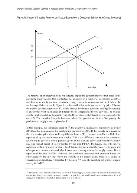
Figure A1: Impact of Subsidy Removal on Output (Example of a Consumer Subsidy in a Closed Economy)
The removal of an energy subsidy will directly impact the equilibrium price that holds in the
particular energy market that is affected. For example, in a number of developing countries
and former centrally planned countries, energy prices to consumers are held below the
market-equilibrium price. In Figure A1, this subsidised price is represented by price P 2 below
the market equilibrium price of P 0 . In this market the demand function, relating the quantity
of energy that will be demanded at different prices, is represented by the curve D. The original
supply function, relating the quantity supplied by producers at different prices, is given by the
curve S. The subsidised supply function, where the government is in effect paying the
producers to supply more, is given by S 1 .
In this example, the subsidised price of P 2 , the quantity demanded by consumers, is greater
(Q 1 ) than that demanded at the equilibrium market price (Q 0 ). If the subsidy is removed so
that the market price rises to the equilibrium level of P 0 , consumers’ welfare will decline,
represented by the loss in consumer surplus. This is the difference between what consumers
are willing to pay for a given quantity (given by the demand curve) and what they actually
pay (the market price). It is represented by the area P 2 P 0 EA. Producers, too, will suffer a
reduction in their producer surplus – the difference between what they receive for each unit
of output (the market price) and what it costs to produce (given by the supply curve). This is
represented by area P 1 P 0 EB. However, the combined consumer and producer losses are
outweighed by the fact that when the subsidy is no longer given, there is a saving in
government expenditure, represented by the area P 2 P 1 BA. The resulting net welfare gain to
society is EAB. 106 156
106 This analysis has been shown for only one market. When supply and demand in different markets are related,
the analysis has to be extended to several markets. In practice, this would require more data on the effects of
changes in prices in one market on demand and supply in others.