Frequency domain design of observers for linear systems using a ...

Frequency domain design of observers for
linear systems using a factorization approach
Montassar Ezzine ∗,∗∗ , Harouna Souley Ali ∗∗ , Mohamed Darouach ∗∗
et Hassani Messaoud ∗
∗∗ Centre de Recherche en Automatique de Nancy (CRAN - UMR 7039)
Nancy-Université - CNRS
IUT de Longwy, 186 rue de Lorraine
54400 Cosnes et Romain, FRANCE
∗ Ecole Nationale d’Ingénieurs de Monastir, Avenue Ibn El Jazzar, 5019 Monastir,
Tunisie
montassarezzine@yahoo.fr; souley@iut-longwy.uhp-nancy.fr; darouach@iut-longwy.uhpnancy.fr;
hassani.messaoud@enim.rnu.tn
Section de rattachement : 61
Secteur : Secondaire
RÉSUMÉ : This paper proposes an easier frequency domain design of observers for linear
systems, where all measurements are not corrupted by disturbances, with the aid of a factorization
approach . The design procedure in the frequency domain is first obtained from the
time domain solution where we use the full order observer of type Luenberger , and then by
the use of the factorization approach where we propose to define some useful coprime factorization,
the representation in the frequency domain is derived. The frequency designed filter
is easy to calculate as it requires only computation of a suitably coprime factorization.
MOTS CLÉS : Time domain, frequency domain, linear system, observer-based controller,
Linear Matrix inequalities (LMIs), Matrix fractions descriptions (MFDs).
1. Introduction
A common feature of control schemes is the assumption that the system
state vector is available for feedback control purposes. The fact that systems
rarely satisfy this assumption necessites the reconstruction of the missing state
variables. So the state observation problem centres on the construction of an
auxiliary dynamic system, known as a state reconstructor or observer, driven
by the available system inputs and outputs. There is many results in time
domain [2], [3], [4], [9], [10] ... Unfortunately there is less literature in frequency
domain although is the basis for most analysis performed on control systems
and it is well known that both linear optimal state feedback and optimal linear
filtering problems can be formulated and solved in the frequency domain. A first
solution for the filter transfer matrix was presented by MacFarlane (1971)[7],
and it was demonstrated in [8] that optimal state feedback low and the optimal
filter can be characterized by polynomial matrix that directly parameterize the
1

state feedback control and the observer in the frequency domain.
In this paper we intend to give a frequency domain description of full order
observers for linear systems where all measurements not corrupted by disturbances,
i.e noise - free output measurements, using the factorization approach
[1]. The procedure of designing such observers is obtained by using the famous
full order observer of type Luenberger designed in time domain [2] , then by
applying the factorization approach, where we propose some useful coprime factorization,
the desired representation in the frequency domain is derived. The
main reason of formulating the results of the time domain in the frequency one,
is the advantages that it presents for the observer-based control [13]. In fact,
in this case, the compensator is driven by the input and the output of the system.
So only the input-output behaviour of the compensator (characterized by
its transfer function) influences the properties of the closed-loop system. The
additional degrees of freedom given by the frequency approach can then be used
for robustness purpose for example [13].
The present work is organized as follows. The next section present the
problem that we propose to solve . Section 3 gives the time domain solution
for this full order problem that will be useful for our frequency domain design,
deduced from [2]. Section 4 deals with twofold . First we review some important
results of the factorization approach , and in a second time, we give the main
result of the paper by proposing a frequency domain description of full order
observer for linear systems . In Section 5 we present an illustrative example and
Section 6 concludes the paper.
2. Problem Statement
Consider the linear time-invariant multivariable system described by
ẋ(t) = Ax(t)+Bu(t) (1a)
y(t) = Cx(t) (1b)
Where x(t) ∈ n and y(t) ∈ m m ≤ n, are the state vector, the output
vector of the system, and u(t) ∈ q represents the input vector. The system
matrices A, B and C assumed to be known.
Problem :
Our aim is to design a full order observer, for system (1) in the frequency
domain using the factorization approach [1]. This frequency domain observer
will generates the estimate ˆx(s) for the Laplace Transform of the state vector
x(t) ,x(s) using the measurements y(s) and the inputs u(s).
3. Full Order observer in the time domain
Before giving the time domain design of the estimator , it is of interest to
recall the following definition:
Définition 1. [2]
2

The state reconstruction problem is one of determining the state x(τ) of the system (1)
at time τ from a knowledge of the output measurements y(σ), σ ≤ τ.
So, by follows that of [2], a full- order observer for the system (1)
described by
can be
˙ˆx(t) = Aˆx(t)+Bu(t)+G(y(t) − ŷ(t)) (2)
where ˆx(t) ∈ n denotes the estimated state and G is the correction gain of
the observer.
Let’s define the estimation error a
Then, the dynamics of this estimation error is
e(t) = x(t) − ˆx(t) (3)
ė(t) = ẋ(t) − ˙ˆx(t) (4)
= (A − GC)e(t) (5)
Therefore, the estimation error can be asymptotically reduced to zero, if and
only if the pair (A, C) is completely observable. In this case, one can choose
the gain G to assign the eigenvalues of the matrix (A- G C) to the left- hand
side of the complex plane.
In the sequel we shall give a frequency domain representation of the full
order observer (2) .
4. Full order observer in the frequency domain
In this section we propose an easier technique of designing observers for
linear systems in the frequency domain. In fact, the procedure design is derived
from time domain results with the aid of the factorization approach [1] after
reviewing some important notations and results.
4.1. Factorization approach: A review
A transfer matrix H(s) is said to be a RH∞ - matrix if H(s) is a real- rational
matrice which is stable and proper. Furthermore, a state- space realization of
H(s) =C(sI − A) −1 B + D (6)
is denoted by
A B C D
(7)
A rational function matrix H(s) is a matrix whose elements are rational functions.
A right polynomial matrix fraction (PMF) for the p × m rational function
matrix H(s) is an expression of the form
H(s) =N(s)M −1 (s) (8)
3

where N(s) is a p × m polynomial matrix, and M(s) is an m × m nonsingular
polynomial matrix. Such a PMF is further called a right coprime PMF if N(s)
and D(s) are right coprime.
A left polynomial matrix fraction for H(s) is an expression of the form
H(s) = ˆM −1 (s) ˆN(s) (9)
where ˆN(s) isap × m polynomial matrix, and ˆM(s) isap × p nonsingular
polynomial matrix. Such a PMF is further called a left coprime PMF if ˆM(s)
and ˆN(s) are right coprime.
Therefore, a double coprime factorization of H(s) reads
H(s) =N(s)M −1 (s) = ˆM −1 (s) ˆN(s) (10)
For this double coprime factorization there exist four polynomial matrices Y(s),
X(s), Ŷ (s) and ˆX(s) satisfying the Bezout identity [1]:
Y (s) X(s) M(s) − ˆX(s)
− ˆN(s) ˆM(s) N(s) Ŷ (s)
M(s) ˆX(s) Y (s) −X(s)
−N(s) Ŷ (s) ˆN(s) ˆM(s)
I 0
0 I
=
=
(11)
Following the algorithm provided in [5] all matrices implemented in the bezout
identity can be realized as follows:
M(s) = A k B K I (12)
N(s) = A k B C + DK D (13)
ˆM(s) = A l −L C I (14)
ˆN(s) = A l B − LD C D (15)
Y (s) = A l B − LD −K I (16)
X(s) = A l L −K 0 (17)
Ŷ (s) = A k L C + DK I (18)
ˆX(s) = A k L −K 0 (19)
where K and L are chosen such that A k = A+BK and A l = A−LC are stable.
4.2. Main results
In this section, based on factorization approach the problem of designing full
order observers in the frequency domain is solved.
Théoreme 1. : A frequency domain representation of the estimated states obtained
from the full-order observer (2) of order n , with the aid of following coprime factorizations
4

i)
(sI − Π) −1 B =
ˆM
−1
1 (s) ˆN 1 (s) (20)
ii)
(sI − Π) −1 G =
ˆM
−1
2 (s) ˆN 2 (s) (21)
with Π=A − GC
is given by,
ˆx(s) =
−1 ˆM 1 (s)( ˆN 1 (s) u(s)+ ˆN 2 (s) y(s)) (22)
Preuve 1. By taking the Laplace transform of (2) we have
which implies that
sˆx(s) =Πx(s)+Bu(s)+Gy(s) (23)
ˆx(s) =(sI − Π) −1 Bu(s)+(sI − Π) −1 Gy(s) (24)
Now, from proposed factorizations, we have:
a)
(sI − Π) −1 B =
ˆM
−1
1 (s) ˆN 1 (s) (25)
with
ˆM 1 (s) = A l −L I I (26)
ˆN 1 (s) = A l B l I 0 (27)
where A l =Π− LC and B l = B − L.0 =B, L is chosen such that A l is
stable.
b)
(sI − Π) −1 G =
ˆM
−1
2 (s) ˆN 2 (s) (28)
with
where G l = G − L0 =G .
ˆM 2 (s) = A l −L I I (29)
= ˆM 1 (s) (30)
ˆN 2 (s) = A l G l I 0 (31)
Substituting equation (25), (28) with (30) in (24), the theorem is immediately proved.
5

5. Numerical Example
Consider the linear system
⎡
ẋ(t) =
y(t) =
⎣ −3 1 0
0 −2 0
0 0 −1
⎡
⎣ 1 0 0
1 1 0
0 1 0
⎤
⎤
⎦ x(t)+
⎡
⎣ 0 0
1
⎤
⎦ u(t)
⎦ x(t) (32)
1 - Time domain design
The full order observer (24) is determined by specifying the observer gain
⎡
G = ⎣ g ⎤
1 g 4 g 7
g 2 g 5 g 8
⎦ (33)
g 3 g 6 g 9
The resulting observer system matrix is
⎡
−3 − g 1 − g 4 −g 4 − g 7 0
⎤
A − GC = ⎣ −g 2 − g 5 −2 − g 5 − g 8 0 ⎦ (34)
−g 3 − g 6 −g 6 − g 9 −1
which has corresponding characteristic equation
We decide to do a pole placement. In fact we want to make the observer
have as eigenvalues -3 and -4 in addition of -1 which is a fixed pole. This would
give the characteristic equation
P 1 (λ) =λ 3 +8λ 2 + 19λ + 12 (35)
So, with a simple identification, we deduce that
⎡
−2 2 ⎤
G = ⎣ −1 1 1 ⎦ (36)
1 −1 0
The observer is thus governed by
˙ˆx(t) =
+
⎡
⎣ −3 0 0
0 −4 0
0 1 −1
⎡
⎣ −1 1 1
2 −2 2
1 −1 0
⎤
⎤
⎦ ˆx(t)+
⎡
⎣ 0 0
1
⎤
⎦ u(t)
⎦ y(t) (37)
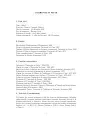
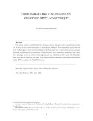
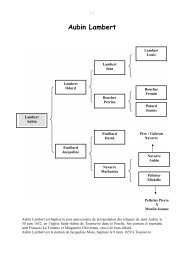
In the following we draw the evolution of the third components of the estimation
error: we take as initial conditions
x(0) = 1 2 1 (38)
ˆx(0) = 0 0 0 (39)
6

1
First component of the estimation error
0.9
0.8
0.7
0.6
Amplitude
0.5
0.4
0.3
0.2
0.1
0
0 1 2 3 4 5 6 7 8
Time (sec)
Figure 1.: The evolution of the first component of the estimation error
2
Second component of the estimation error
1.8
1.6
1.4
1.2
Amplitude
1
0.8
0.6
0.4
0.2
0
0 1 2 3 4 5 6 7 8
Time (sec)
Figure 2.: The evolution of the second component of the estimation error
2 - Frequency domain design
We intend therefore in this section to find the polynomial matrices ˆM 1 (s), ˆN1 (s)
and ˆN 2 (s) with the aid of the factorization approach.
1) From (26), we have ˆM 1 (s) = A l −L I I with A l =Π− LC.
we choose
⎡
L = ⎣
2 −1 1
3 −3 1
−2 2 −1
⎤
⎦ (40)
so that
A l =
⎡
⎣ −4 0 0
0 −2 0
0 0 −1
⎤
⎦ (41)
7

1
Third component of the estimation error
0.9
0.8
0.7
0.6
Amplitude
0.5
0.4
0.3
0.2
0.1
0
0 1 2 3 4 5 6 7 8
Time (sec)
Figure 3.: The evolution of the third component of the estimation error
which is stable. So,
⎡
⎣
s+2
s+4
−3
s+2
2
s+1
ˆM 1(s)
=
1
s+4
s+5
s+2
−2
s+1
−1
s+4
−1
s+2
s+2
s+1
−1
and therefore, ˆM 1 (s) needed in the frequency domain design reads
⎡
⎢
⎣
s 3 +11s 2 +36s+32
s 3 +9s 2 +27s+24
3s 2 +16s+16
s 3 +9s 2 +27s+24
−2s 2 −12s−16
s 3 +9s 2 +27s+24
ˆM −1
1 (s)
=
−s 2 −2s
s 3 +9s 2 +27s+24
s 3 +6s 2 +14s+12
s 3 +9s 2 +27s+24
2s 2 +10s+12
s 3 +9s 2 +27s+24
⎤
⎦
s 2 +5s+4
s 3 +9s 2 +27s+24
s 2 +6s+5
s 3 +9s 2 +27s+24
s 3 +8s 2 +20s+13
s 3 +9s 2 +27s+24
⎤
⎥
⎦
(42)
(43)
2) From (27), ˆN1 (s) = A l B l I 0 with B l = B. So,
⎡ ⎤
0
ˆN 1 (s) = ⎣ 0 ⎦ (44)
1
s+1
3) From (31), ˆN2 (s) = A l G l I 0 with G l = G. So,
⎡
⎤
ˆN 2 (s) = ⎣
2
s+4
−1
s+2
1
s+1
−2 2
s+4 s+4
1 1
s+2 s+2
−1
s+1
0
⎦ (45)
Following (43), (44) and (45) the proposed frequency domain observer (22)
holds.
Finally we propose to draw , as the time domain case, the behavior of the
frequency estimation error.
For that, from (22), it is readily follows that
ˆx(s) = M 0 u(s) (46)
8

with
⎡
⎢
⎣
M 0
=
s 2 +5s+4
(s 3 +9s 2 +27s+24)(s+1)
s 2 +6s+5
(s 3 +9s 2 +27s+24)(s+1)
s 3 +8s 2 +20s+13
(s 3 +9s 2 +27s+24)(s+1)
⎤
⎥
⎦
(47)
and therefore the estimation error designed in the frequency domain reads
e(s) = x(s) − ˆx(s) (48)
= ((sI − A) −1 B − M 0 )u(s) (49)
⎡
⎤
=
⎢
⎣
s 2 +5s+4
(s 3 +9s 2 +27s+24)(s+1)
s 2 +6s+5
(s 3 +9s 2 +27s+24)(s+1)
s 3 +8s 2 +20s+13
(s 3 +9s 2 +27s+24)(s+1)
⎥
⎦
u(s) (50)
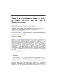
Finally, we draw in figure 4, 5, 6 the evolution of the three frequency estimation
error and its impulse response in figure 7, 8 and 9 to show the effectiveness of
proposed approach.
6. Conclusion
We developed in this paper, using the factorization approach, an easier frequency
domain design of full order observers where linear systems with measurements
not corrupted by disturbances, i.e noise - free output measurements is
considered. The design procedure is obtained from the full order observer of type
Luenberger designed in time domain , then applying the factorization approach,
where we propose some useful coprime factorization, the desired representation
in the frequency domain is derived. The frequency designed observer is easy
to calculate as it requires only computation of a suitably coprime factorization.
The proposed full order observer has been carried on a numerical example and
the results were successful. The further works will concern the design of observers
for descriptor systems in the frequency domain and the observer-based
compensator design as it is the main motivation of the frequency domain approach
[13].
References
[1] : Vidyasagar.M, ”Control Systems Synthesis: A Factorization Approach”,M.I.T,Press,
Cambridge, MA,1985.
[2] : O’Reilly.J, ”Observers for Linear Systems”, New York, NY: Academic,
1983.
[3] : D. G. Luenberger, ”Observers for multivariable systems”, IEEE
Trans.Automat. Contr., vol. 11, pp. 190-197, 1966.
[4] : D. G. Luenberger, , ”An introduction to observers”, IEEE Trans. Automat.
Contr., vol. 16, pp. 596-602, 1971.
9

[5] : Francis.B.A, ”A Course in H ∞ Control Theory. Springer-Verlag, Berlin-
New York,1987.
[6] : Antsaklis.P and Michel.N, ”Linear Systems ”, New York: McGraw-Hill,
1997.
[7] : MacFarlane,A.G.J, ”Return-difference matrix properties for optimal stationary
Kalman-Bucy filter”, Proceedings of the Institution of Electrical
Engineers, 118, 373-376 1971.
[8] : Anderson.B.D.O and Ku˘cera.V , ”Matrix fraction construction of linear
compensators”, IEEE Transaction on Automatic Control.Processing, 30,
1112-1114 1985.
[9] : Darouach M., Zasadzinski M., Xu S.J.,, ”Full- order observers for linear
systems with unknown inputs”, IEEE Trans. Automat. Contr., vol AC. 39,
pp. 606-609, 1994.
[10] : Battacharyya S.P.,, ”Observer design for linear systems with unknown
inputs”, IEEE Trans. Automat. Contr., vol AC. 23, pp. 483-484, 1978.
[11] : Ding.X, Frank.M.P and Guo.L, ”Robust Observer Design Via Factorization
Approach”, Proceedings of the 29th Conlerence on Decioion and
Control Honolulu. Hawall December 1990.
[12] : Ding.X, Guo.L and Frank.M.P , ”Parameterization of Linear Observers
and Its Application to Observer Design”, IEEE Transaction on Automatic
Control.Processing, 39, 1648-1652 1994.
[13] : Hippe.P and Deutscher.J, ”Design of observer-based compensators : From
the time to the frequency domain”, Springer-Verlag, London, 2009.
[14] : Markez. H. J, ”A frequency domain approach to state estimation”, Journal
of the Franklin Institute 340, 147-157 , 2003.
0
Bode diagram of the first component of the frequency estimation error e(s)
−10
−20
Magnitude (dB)
−30
−40
−50
−60
−70
−80 180
135
Phase (deg)
90
45
0
10 −2 10 −1 10 0 10 1 10 2
Frequency (rad/sec)
Figure 4.: The Bode diagram of the first component of the frequency estimation error
10

−80
0
Bode diagram of the second component of the frequency estimation error e(s)
−10
−20
Magnitude (dB)
−30
−40
−50
−60
−70
180
135
Phase (deg)
90
45
0
10 −2 10 −1 10 0 10 1 10 2
Frequency (rad/sec)
Figure 5.: The Bode diagram of the second component of the frequency estimation
error
0
Bode diagram of the third component of the frequency estimation error e(s)
−10
−20
Magnitude (dB)
−30
−40
−50
−60
−70
−800
−45
Phase (deg)
−90
−135
−180
10 −2 10 −1 10 0 10 1 10 2
Frequency (rad/sec)
Figure 6.: The Bode diagram of the third component of the frequency estimation error
0
Impulse response of the first component of the frequency estimation error e(s)
−0.02
−0.04
−0.06
Amplitude
−0.08
−0.1
−0.12
−0.14
−0.16
0 0.5 1 1.5 2 2.5 3 3.5 4
Time (sec)
Figure 7.: The impulse response of the first component of the frequency estimation
error
11

0 0.5 1 1.5 2 2.5 3 3.5 4
0
Impulse response of the second component of the frequency estimation error e(s)
−0.02
−0.04
−0.06
Amplitude
−0.08
−0.1
−0.12
−0.14
−0.16
−0.18
Time (sec)
Figure 8.: The impulse response of the second component of the frequency estimation
error
0.25
Impulse response of the third component of the frequency estimation error e(s)
0.2
0.15
Amplitude
0.1
0.05
0
0 1 2 3 4 5 6
Time (sec)
Figure 9.: The impulse response of the third component of the frequency estimation
error
12