Using Cumulative Count Of Conforming CCC-Chart to Study the ...

8
6-2 Quesenberry’s Q-Transformation
Using Q -1 to denote the inverse function of standard normal distribution, define
Q
i
= −Q
where
−1
( u )
i
xi ui
= F(
xi
, p)
= 1−
(1 − p)
For i = 1,2,3 ,.... Qi
Will approximately follow the standard normal distribution, and the accuracy
improves as p approaches zero.
Table (6-4) shows the data of Quesenberry’s Transformation of CCC-EXP data
Q i Q i Q i Q i
0.2327 2.326 0.7507 0.7621
-0.2611 2.326 2.326 0.9385
2.326 0.1257 2.326 -0.2224
2.326 1.0494 2.326 1.0494
0.628 2.326 2.326 0.7507
2.326 0.7507 -1.165 2.326
2.326 2.326 -1.2873 1.0494
0.4316 -1.165 1.4532 1.0494
0.628 -0.3836 0.0426 2.326
-0.831 2.326 0.9002 2.326
0.7507
5.8
X Chart for Quesenberry
3.8
UCL = 4.31
X
1.8
-0.2
CTR = 1.10
-2.2
LCL = -2.10
0 10 20 30 40 50
Observation
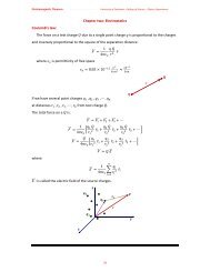
Fig(6-4) The individual chart of CCC_EXP data with Q- Transformation
From above chart of Q- Transformation, it shows that all points are within the
control limits and the process is in control.