Using Cumulative Count Of Conforming CCC-Chart to Study the ...
Using Cumulative Count Of Conforming CCC-Chart to Study the ...
Using Cumulative Count Of Conforming CCC-Chart to Study the ...

You also want an ePaper? Increase the reach of your titles
YUMPU automatically turns print PDFs into web optimized ePapers that Google loves.
1<br />
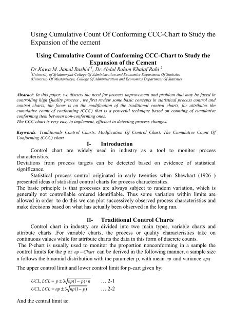
<strong>Using</strong> <strong>Cumulative</strong> <strong>Count</strong> <strong>Of</strong> <strong>Conforming</strong> <strong>CCC</strong>-<strong>Chart</strong> <strong>to</strong> <strong>Study</strong> <strong>the</strong><br />
Expansion of <strong>the</strong> cement<br />
<strong>Using</strong> <strong>Cumulative</strong> <strong>Count</strong> of <strong>Conforming</strong> <strong>CCC</strong>-<strong>Chart</strong> <strong>to</strong> <strong>Study</strong> <strong>the</strong><br />
Expansion of <strong>the</strong> Cement<br />
Dr.Kawa M. Jamal Rashid 1 , Dr.Abdul Rahim Khalaf Rahi 2<br />
1 University of Sylaimanyah College <strong>Of</strong> Administration and Economics Department <strong>Of</strong> Statistics @<br />
2University <strong>Of</strong> Mustanisirya, College <strong>Of</strong> Administration and Economics Department <strong>Of</strong> Statistics<br />
Abstract: In this paper, we discuss <strong>the</strong> need for process improvement and problem that may be faced in<br />
controlling high Quality process , we first review some basic concepts in statistical process control and<br />
control charts, <strong>the</strong> focus is on <strong>the</strong> modification of <strong>the</strong> traditional control charts, for attributes <strong>the</strong><br />
cumulative count of conforming (<strong>CCC</strong>) that is a powerful technique based on counting of cumulative<br />
conforming item between non-conforming ones.<br />
The <strong>CCC</strong> chart is very easy <strong>to</strong> implement, efficient in detecting process changes.<br />
Keywords: Traditionals Control <strong>Chart</strong>s. Modification <strong>Of</strong> Control <strong>Chart</strong>, The <strong>Cumulative</strong> <strong>Count</strong> <strong>Of</strong><br />
<strong>Conforming</strong> (<strong>CCC</strong>) chart<br />
I- Introduction<br />
Control chart are widely used in industry as a <strong>to</strong>ol <strong>to</strong> moni<strong>to</strong>r process<br />
characteristics.<br />
Deviations from process targets can be detected based on evidence of statistical<br />
significance.<br />
Statistical process control originated in early twenties when Shewhart (1926 )<br />
presented ideas of statistical control charts for process characteristics.<br />
The basic principle is that processes are always subject <strong>to</strong> random variation, which is<br />
generally not controllable ordered identifiable. Thus some variation within limits are<br />
allowed in order <strong>to</strong> do this we can plot successively observed process characteristics and<br />
make decisions based on what has actually been observed in <strong>the</strong> long run.<br />
II- Traditional Control <strong>Chart</strong>s<br />
Control chart in industry are divided in<strong>to</strong> two main types, variable charts and<br />
attribute charts .For variable charts, <strong>the</strong> process or quality characteristics take on<br />
continuous values while for attribute charts <strong>the</strong> data in this form of discrete counts.<br />
The P-chart is usually used <strong>to</strong> moni<strong>to</strong>r <strong>the</strong> proportion nonconforming in a sample <strong>the</strong><br />
control limits for <strong>the</strong> p or np − <strong>Chart</strong> can be derived in <strong>the</strong> following manner, a sample size<br />
n follows <strong>the</strong> binomial distribution with <strong>the</strong> parameter p, with mean np and variance npq<br />
The upper control limit and lower control limit for p-cart given by:<br />
UCL , LCL p ± 3 np(1<br />
− p)<br />
/ n<br />
= … 2-1<br />
= np ± 3 np(1<br />
− ) … 2-2<br />
UCL, LCL<br />
p<br />
And <strong>the</strong> central limit is:
2<br />
Cl =<br />
p<br />
And for np-chart, which is used for <strong>the</strong> moni<strong>to</strong>ring number of non-conforming items in<br />
samples of size n ,modified limits are as follows:.<br />
UCL, LCL = np ± 3 np(1<br />
− p)<br />
…2-3<br />
Cl = np<br />
When <strong>the</strong> sample size is fixed for all sample <strong>the</strong> p − chart and np − <strong>Chart</strong> are very<br />
similar and <strong>the</strong> different is only in <strong>the</strong> scale of <strong>the</strong> y-axis. Different p-charts can be easily<br />
compared as <strong>the</strong> center line for <strong>the</strong> process fraction nonconforming level .For np –<strong>Chart</strong><br />
<strong>the</strong> center line is affected by <strong>the</strong> sample size.<br />
When p or<br />
skewness of binomial distribution, <strong>the</strong> lower limit based on 3 sigma concept may not exist<br />
as it is usually a negative value, probability limit should be used when possible .On <strong>the</strong><br />
o<strong>the</strong>r hand, simple modification can be used <strong>to</strong> obtain better control limit for p<br />
or<br />
np − <strong>Chart</strong> .<br />
np − <strong>Chart</strong> are used it is important <strong>to</strong> use <strong>the</strong> appropriate limit, because of <strong>the</strong><br />
II- Modification <strong>Of</strong> Control <strong>Chart</strong><br />
Some improvement made on traditional p and np − <strong>Chart</strong> using some transformations<br />
so as <strong>to</strong> achieve high power in detecting np –words shift in a process, with a simple<br />
adjustments <strong>to</strong> <strong>the</strong> control limits of <strong>the</strong> p-chart one can achieve equal or even better results<br />
form of <strong>the</strong> available methods are as follows:<br />
3-1-Binomial Q chart:<br />
By transforming <strong>the</strong> binomial variable <strong>to</strong> standard normal variable, a Q-chart<br />
(Quesenberry 1997),could be drawn, with upper and lower control limits equal <strong>to</strong> 3 and -3<br />
respectively it is defined by:<br />
And<br />
u<br />
⎛ n ⎞<br />
i<br />
k n−k<br />
i<br />
= ∑ ⎜ ⎟p<br />
(1 − p)<br />
k = 0 p<br />
⎝<br />
⎠<br />
−1<br />
Q i<br />
= φ ( u i<br />
)<br />
−1<br />
Where (.)<br />
…3-1<br />
φ is <strong>the</strong> inverse function of <strong>the</strong> standard normal variable.<br />
Plotting φi<br />
s on <strong>the</strong> char, standard normal control chart with a uniform limit of (0 and 1)<br />
could be maintained.<br />
3-2- Arcsine p-chart<br />
This is ano<strong>the</strong>r nonlinear transformation like in <strong>the</strong> binomial Q chart with<br />
W<br />
i<br />
=<br />
⎡<br />
⎢<br />
⎢sin<br />
⎢<br />
⎢<br />
⎣<br />
⎛<br />
⎜<br />
⎜<br />
⎜<br />
⎜<br />
⎝<br />
3 ⎞<br />
x + ⎟<br />
8 ⎟ − sin<br />
3 ⎟<br />
ni<br />
+ ⎟<br />
8 ⎠<br />
⎤<br />
⎥<br />
⎥<br />
⎥<br />
⎥<br />
⎦<br />
( p )<br />
i<br />
−1<br />
−1<br />
2 ni<br />
…3-2
3<br />
Since W<br />
i<br />
is <strong>the</strong> approximately standard normal, a chart could be drawn by plotting<br />
W on <strong>the</strong> chart with control limits are of 3 and -3 .<br />
i<br />
3-3- Cornish Fisher expansion method.<br />
This method having some additional constant values in <strong>the</strong> three sigma limits using<br />
<strong>the</strong> normal distribution.<br />
Define Yi = X<br />
i<br />
/ n Plotting Y i values on <strong>the</strong> chart it is very easy <strong>to</strong> detect <strong>the</strong> changes in<br />
p values with <strong>the</strong> following control limit<br />
P(1<br />
− P)<br />
4(1 − 2P)<br />
UCL,<br />
LCL = P ± 3 +<br />
…3-3<br />
n 3n<br />
When <strong>the</strong> p is unknown, <strong>the</strong>y have <strong>to</strong> be estimated and inserted in <strong>the</strong> above equations.<br />
It is noted that <strong>the</strong> above equations could be used for variable sample sizes replacing n=n i<br />
3-4-Modified limits for np-<strong>Chart</strong><br />
Ryan and Schwertman (1997) proposed <strong>the</strong> following regression equations of np<br />
and np and found <strong>the</strong>m accurate. The proposed control limits are.<br />
UCL = 0 .6195 + 1.00523np<br />
+ 2. 983 np …3-4<br />
UCL = 2.9529<br />
+ 1..01956np<br />
− 3. 2729 np …3-5<br />
It is noted that <strong>the</strong>se limits are valid for (p
4<br />
V- Setting up of <strong>the</strong> <strong>CCC</strong> chart :<br />
The setting of <strong>the</strong> <strong>CCC</strong> chart is similar <strong>to</strong> <strong>the</strong> generic procedure of <strong>the</strong> setting up a<br />
Shewarthart control chart except that <strong>the</strong> measurement are <strong>the</strong> number of conforming<br />
items after <strong>the</strong> last nonconforming one . This count should be plotted only when a new<br />
conforming item is observed.<br />
Let (n) be <strong>the</strong> number of items observed before a nonconforming one is found i.e (n-1)<br />
items are conforming followed by n th item which is nonconforming .it is clear that this<br />
count follows a geometric distribution. The determination of <strong>the</strong> control limits based on<br />
this.@<br />
If <strong>the</strong> probability nonconforming item is equal <strong>to</strong> p <strong>the</strong>n <strong>the</strong> probability of getting<br />
(n-1) conforming ones following a nonconforming one is :<br />
n−1<br />
p (1 − p)<br />
n= 1,2,… …5-1<br />
The mean of geometric distribution with parameter p which can be used as <strong>the</strong> center line<br />
is :<br />
CL = 1/<br />
P @ …5-2<br />
Suppose that <strong>the</strong> acceptable of false alarm probability is α ,<strong>the</strong> UCL and LCL can be<br />
determined as :<br />
ln( α / 2)<br />
UCL =<br />
@@@@@@@@@@@@@@<br />
…5-3<br />
and<br />
ln(1 − p)<br />
ln(1 − ( α / 2))<br />
LCL =<br />
ln(1 − p)<br />
@ …5-4@ @<br />
Respectively control charts can be set up by including <strong>the</strong> control limits and <strong>the</strong> central<br />
line.<br />
If <strong>the</strong> proportion of non-conforming items a associated with <strong>the</strong> process is p, <strong>the</strong>n<br />
<strong>the</strong> probability that no nonconforming item is found in n inspected is<br />
P(no nonconforming in n items )=(1-P) n …4-5<br />
This prob. reflects <strong>the</strong> certainty we have when we judge <strong>the</strong> process <strong>to</strong> be out of control<br />
when a nonconforming item has been found. Xie and Goh (1992) introduced <strong>the</strong> concept<br />
of certainty level S,<br />
which is <strong>the</strong> probability that <strong>the</strong> process is actually out of control.<br />
The certainty level , S related <strong>to</strong> false alarm probability when interpreting <strong>CCC</strong><br />
chart signal . With one side control limit<br />
S=1- α<br />
…5-6<br />
The relation between <strong>the</strong> proportion of nonconforming items P and number of items<br />
inspected n which is given as:@<br />
( 1− p)<br />
n = S<br />
....5-7<br />
We can now determine <strong>the</strong> number of conforming items inspected before a nonconforming<br />
one is allowed for <strong>the</strong> process <strong>to</strong> still be considered in control, this can be calculated as:<br />
@@@@@@@@@@@@@@@@@@
5<br />
n<br />
ln S<br />
ln(1 − p)<br />
= ….. 5-8<br />
For practical applications a decision graph can be constructed <strong>to</strong> facilitate decisions<br />
on <strong>the</strong> state of control of process whenever nonconforming item is observed.<br />
VI- Application<br />
The important fac<strong>to</strong>r that describe <strong>the</strong> quality of <strong>the</strong> cement is <strong>the</strong> (expansion of <strong>the</strong><br />
cement - EXP) where <strong>the</strong> standard value of this feature is less than 10 mm. A set of <strong>CCC</strong><br />
data is shown in table (5-1)<br />
Table (5-1) shows that <strong>the</strong> cumulative data. With acceptable value of EXP is
6<br />
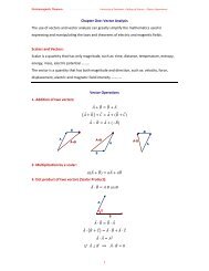
Table(6-2) shows that <strong>the</strong> frequency of occurrence of <strong>the</strong> 17 unique <strong>the</strong> classes are sorted<br />
according <strong>to</strong> <strong>the</strong> counts, with <strong>the</strong> most frequently occurring class first. The highest class is<br />
0 with a count of 16, which represents 39.0244% of <strong>the</strong> <strong>to</strong>tal, and Fig(6-2) shows <strong>the</strong><br />
Pare<strong>to</strong> chart.<br />
Table(6-2) Pare<strong>to</strong> <strong>Cumulative</strong> Frequencies of <strong>CCC</strong>-EXP data<br />
Cusum<br />
Class<br />
CuSum Percent<br />
Rank <strong>Count</strong><br />
Percent<br />
Label<br />
Score %<br />
%<br />
0 1 16 16 39.02 39.02<br />
3 2 4 20 9.76 48.78<br />
1 3 4 24 9.76 58.54<br />
41 4 2 26 4.88 63.41<br />
6 5 2 28 4.88 68.29<br />
4 6 2 30 4.88 73.17<br />
51 7 1 31 2.44 75.61<br />
45 8 1 32 2.44 78.05<br />
31 9 1 33 2.44 80.49<br />
20 10 1 34 2.44 82.93<br />
18 11 1 35 2.44 85.37<br />
17 12 1 36 2.44 87.8<br />
13 13 1 37 2.44 90.24<br />
12 14 1 38 2.44 92.68<br />
10 15 1 39 2.44 95.12<br />
8 16 1 40 2.44 97.56<br />
5 17 1 41 2.44 100<br />
Total 41<br />
Fig(6-2) Pare<strong>to</strong> <strong>Chart</strong> OF <strong>CCC</strong>-EXP data Transformation:
7<br />
The transformation is useful when <strong>the</strong> distribution is non-normal which <strong>the</strong> case for<br />
geometric distribution is. Under <strong>the</strong> transformation, <strong>the</strong> data become normally distributed.<br />
There are a number of transformations available, few of <strong>the</strong>re are shows below:<br />
1-The double square root Transformation<br />
A double square root for <strong>the</strong> (fourth root) is a simple transformation by:<br />
(0.25)<br />
Y = X , X ≥ 0<br />
The below table Show that <strong>the</strong> illustrate some possible transformation approaches.<br />
Table (6-3) Transformations of <strong>CCC</strong>-EXP data<br />
(0.25)<br />
Y = X<br />
(0.25)<br />
(0.25)<br />
Ln(x) Y = X Ln(x) Y = X Ln(x)<br />
(0.25)<br />
Y = X Ln(x)<br />
1.778 2.303 0 1.000 1.495 1.609<br />
2.060 2.890 0 0 1.414 1.386<br />
0 1.861 2.485 0 2.031 2.833<br />
0 1.316 1.099 0 1.316 1.099<br />
1.565 1.792 0 0 1.000 0<br />
0 1.000 0 2.530 3.714 0<br />
0 0 2.590 3.807 1.316 1.099<br />
1.682 2.079 2.530 3.714 2.672 3.932 1.316 1.099<br />
1.565 1.792 2.115 2.996 1.899 2.565 0<br />
2.360 3.434 0 1.414 1.386 0<br />
1<br />
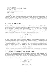
In Fig(6-3)<strong>the</strong> corresponding <strong>CCC</strong> chart is displayed in this case , all points are within <strong>the</strong><br />
control limits and <strong>the</strong> process is in control compare with fig.(6-2)<br />
Fig(6-3) The of Transformation data chart of <strong>CCC</strong>_EXP
8<br />
6-2 Quesenberry’s Q-Transformation<br />
<strong>Using</strong> Q -1 <strong>to</strong> denote <strong>the</strong> inverse function of standard normal distribution, define<br />
Q<br />
i<br />
= −Q<br />
where<br />
−1<br />
( u )<br />
i<br />
xi ui<br />
= F(<br />
xi<br />
, p)<br />
= 1−<br />
(1 − p)<br />
For i = 1,2,3 ,.... Qi<br />
Will approximately follow <strong>the</strong> standard normal distribution, and <strong>the</strong> accuracy<br />
improves as p approaches zero.<br />
Table (6-4) shows <strong>the</strong> data of Quesenberry’s Transformation of <strong>CCC</strong>-EXP data<br />
Q i Q i Q i Q i<br />
0.2327 2.326 0.7507 0.7621<br />
-0.2611 2.326 2.326 0.9385<br />
2.326 0.1257 2.326 -0.2224<br />
2.326 1.0494 2.326 1.0494<br />
0.628 2.326 2.326 0.7507<br />
2.326 0.7507 -1.165 2.326<br />
2.326 2.326 -1.2873 1.0494<br />
0.4316 -1.165 1.4532 1.0494<br />
0.628 -0.3836 0.0426 2.326<br />
-0.831 2.326 0.9002 2.326<br />
0.7507<br />
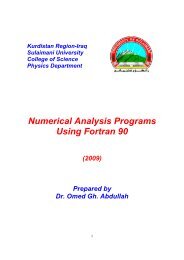
5.8<br />
X <strong>Chart</strong> for Quesenberry<br />
3.8<br />
UCL = 4.31<br />
X<br />
1.8<br />
-0.2<br />
CTR = 1.10<br />
-2.2<br />
LCL = -2.10<br />
0 10 20 30 40 50<br />
Observation<br />
Fig(6-4) The individual chart of <strong>CCC</strong>_EXP data with Q- Transformation<br />
From above chart of Q- Transformation, it shows that all points are within <strong>the</strong><br />
control limits and <strong>the</strong> process is in control.
9<br />
6-3 Finding <strong>the</strong> Sample Size at different fractional non conforming level at<br />
certainly level of S:<br />
To find <strong>the</strong> Sample Size at different fractional non conforming level at certainly<br />
level of S value by using <strong>the</strong> equation (5-7 and 5-8) and depend on <strong>the</strong> P, and S value it<br />
seen <strong>the</strong> result in <strong>the</strong> below table (6-5).<br />
We give some numerical values of (n) for some different combinations of values of p and<br />
S. If <strong>the</strong> cumulated count of conforming item is less than <strong>the</strong> tabulated value , <strong>the</strong>n <strong>the</strong><br />
proportion of nonconforming items is higher than with certainty S.<br />
This table can be used <strong>to</strong> determine <strong>the</strong> value of certainty level (s) for a given level<br />
of proportion nonconforming P , as well as determine <strong>the</strong> value of (p) for given level of<br />
certainty and see if it is higher than <strong>the</strong> acceptable level for <strong>the</strong> process .Fur <strong>the</strong>re more for<br />
given (p and s ), determine <strong>the</strong> minimum number of conforming item that must have been<br />
observed before a nonconforming one can be <strong>to</strong>lerate ie , <strong>the</strong> process can still be deemed<br />
under control even one nonconforming item has been observed.<br />
Table (6-5) Sample Size at different fractional non conforming level<br />
P value<br />
S=1-α<br />
If<br />
S 1 =0.90<br />
<strong>the</strong>n n<br />
If<br />
S 2 =0.95<br />
<strong>the</strong>n n<br />
If<br />
S 3 =0.98<br />
<strong>the</strong>n n<br />
0.001<br />
105.308<br />
51.268<br />
20.193<br />
0.002<br />
52.628<br />
25.621<br />
10.091<br />
0.003<br />
35.067<br />
17.072<br />
6.724<br />
0.004<br />
26.287<br />
12.798<br />
5.041<br />
0.005<br />
21.019<br />
10.233<br />
4.030<br />
0.006<br />
17.507<br />
8.523<br />
3.357<br />
0.007<br />
14.999<br />
7.302<br />
2.876<br />
0.008<br />
13.117<br />
6.386<br />
2.515<br />
0.009<br />
11.654<br />
5.674<br />
2.235<br />
0.01<br />
10.483<br />
5.104<br />
2.010<br />
0.011<br />
9.525<br />
4.637<br />
1.826<br />
0.012<br />
8.727<br />
4.249<br />
1.673<br />
0.013<br />
8.052<br />
3.920<br />
1.544<br />
0.014<br />
7.473<br />
3.638<br />
1.433<br />
0.016<br />
6.532<br />
3.180<br />
1.253<br />
0.018<br />
5.801<br />
2.824<br />
1.112<br />
0.02<br />
5.215<br />
2.539<br />
1.000
10<br />
Fig( 6-5) A decision graph for <strong>the</strong> stat of control of a process<br />
Fig (5-5) Show <strong>the</strong> chart of <strong>the</strong> sample size of different fractional non conforming level at<br />
certainty level, s Number <strong>Of</strong> –non- conforming items percent non conforming.<br />
Since usually p
[8]. Kemp, K.W. (1962) Applied Statistics, Vol. 11, pp. 16–31, ‘The use of cumulative sums for sampling inspection<br />
schemes.’<br />
[9]. Xie ,TN Goh, V Kuralmani (2002)Statistical Model And Control <strong>Chart</strong> For High- Quality Process.<br />
[10]. Oakland, J.S.(2000) Total Quality Management – Text and Cases, 2nd Edition, Butterworth -Heinemann, Oxford,<br />
UK.<br />
[11]. Ognyan Ivanov 2011 APPLICATIONS AND EXPERIENCES OF QUALITY CONTROL<br />
[12]. PETER W. M. JOHN (1990) Statistical Methods in Engineering and Quality Assurance<br />
[13]. Xie, M: Goh T.N and tang X,Y(2000) Data Transformation for geometrically distributed quality characteristics<br />
[14]. Yang , Z.I : Xie M and Goh (2000) Process moni<strong>to</strong>ring of exponentially distributed characteristics through an optimal<br />
normalizing transformation .<br />
@@@@@@<br />
@@<br />
11