New metrics for rigid body motion interpolation - helix

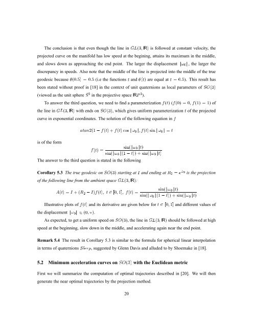
The conclusion is that even though the line in GL(3; IR) is followed at constant velocity, the
projected curve on the manifold has low speed at the begining, attains its maximum in the middle,
and slows down as approaching the end point. The larger the displacement k! 0 k, the larger the
discrepancy in speeds. Also note that the middle of the line is projected into the middle of the true
geodesic because (0:5) = 0:5 (i.e the functions t and (t) are equal at t = 0:5). This result has
been stated without proof in [18] in the context of unit quaternions as local parameters of SO(3)
(viewed as the unit sphere S 3 in the projective space IRP 3 ).
To answer the third question, we need to find a parameterization f (t) (f (0) = 0, f (1)=1)of
the line in GL(3; IR) with ends on SO(3), which gives uniform parameterization t of the projected
curve in exponential coordinates. The solution of the following equation in f
atan2(1 , f (t) +f (t) cos k! 0 k;f(t) sin k! 0 k = t
is of the form
sin(k! 0 kt)
f (t) =
sin(k! 0 k(1 , t)) + sin(k! 0 kt)
The answer to the third question is stated in the following
Corollary 5.3 The true geodesic on SO(3) starting at I and ending at R 2 = e^! 0
is the projection
of the following line from the ambient space GL(3; IR):
A(t) =I +(R 2 , I)f (t); t 2 [0; 1]; f (t) =
sin(k! 0 kt)
sin(k! 0 k(1 , t)) + sin(k! 0 kt)
Illustrative plots of f (t) and its derivative are given below for t 2 [0; 1] and different values of
the displacement k! 0 k2(0;).
As expected, to get a uniform speed on SO(3), the line in GL(3; IR) should be followed at high
speed at the beginning, slow down in the middle, and accelerating again near the end point.
Remark 5.4 The result in Corollary 5.3 is similar to the formula for spherical linear interpolation
in terms of quaternions Slerp, suggested by Glenn Davis and alluded to by Shoemake in [18].
5.2 Minimum acceleration curves on SO(3) with the Euclidean metric
First we will summarize the computation of optimal trajectories described in [20]. We will then
generate the near optimal trajectories by the projection method.
20