Three Problems in Robotics - helix

Three Problems in RoboticsJ.M. SeligSchool of Computing, Info. Sys. & Maths.South Bank UniversityLondon SE1 0AA, U.K.AbstractThree rather different problems in robotics are studied using the same technique from screwtheory. The first problem concerns systems of springs. We differentiate the potential functionin the direction of an arbitrary screw to find the equilibrium position. The second problem isalmost identical in terms of the computations, we seek the least squares solution to the problemof finding the rigid motion undergone by a body given only data about points on the body. Finallywe look at the Jacobian of a Stewart platform. Six point on the moving platform are connectedby prismatic joints to six fixed points on the base. The Jacobian relates the joint rates of the legsto the linear and angular velocities of the platform. Again this can be done by differentiatingwith respect to a screw.Although all three problems are quite well known and have be solved by other means, thescrew theory method is significantly simpler. For example, when minimising a potential orresidual function we do not need to include constraints. These advantages mean that we can gofurther and study second order properties, the Hessian of the spring system, whether or not theleast squares solution minimises or maximises the residual.1 IntroductionWhen Ball wrote his treatise at the end of the 19th centaury Sophius Lie was justbeginning to think about what he called ‘continuous groups’. If Ball knew of Lie’swork it may not have been obvious that it had any connection to his own since Lie wasinterested in symmetries of differential equations. It was Klien who later introducedthe idea that these ‘Lie groups’ could be thought of as geometrical symmetries. It wasafter both Ball and Lie had died that ‘Lie theory’ began to finds it place as central tomodern geometry. In particular, the work of Killing and Cartan on Lie algebras werevery influential.With hindsight we can see that Ball’s finite screws were simply elements of a Liegroup: the group of proper Euclidean transformations in IR 3 .1

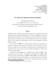
λ iaibiFigure 1: A Rigid Body Suspended by a System of SpringsThe infinitesimal screws or motors were elements of the Lie algebra of this group.Many other elements of Lie theory were also present in Ball’s screw theory. But perhapstheir significance was not fully appreciated. For example, the Lie product or Liebracket is simply the cross product of screws. For Ball this was just a geometricaloperation, the analogue of the vector product of 3-dimensional vectors.Some authors refer to Screw theory and Lie group methods as if they were differentapproaches. This author’s view is that there is no distinction between them, screwtheory is simply the specialisation of Lie theory to the group of rigid body transformations.The name screw theory is useful in three ways, it is a useful shorthand, it isdescriptive and lastly it reminds us that it was Ball who worked out almost all of thetheory before Lie groups were invented!In this work the fact that a Lie group is a differential manifold is used. To minimisea smooth function on such a space we do not need the machinery of Lagrange multipliers.We can work on the manifold directly, we do not need to think of the group asembedded in Cartesian space, as would be implied by the use of Lagrange multipliers.To find equations for a function’s stationary points we differentiate along tangentvector fields. The most convenient vector fields to use are the left-invariant fields onthe group. These are just elements of the Lie algebra of the group, the screws. Hencethis technique could be thought of as, “differentiating along a screw”.2 SpringsConsider a rigid body supported by a system of springs, see figure 1. Further assumethat the springs have natural length 0, obey Hook’s law and can both push and pull. Thespring constants λ i , of the springs can be different. Let ã T i =(a T i , 1) be the points wherethe springs are attached to the ground or frame, and ˜b T i =(b T i , 1) the correspondingattachment points on the rigid body when the body is in some standard ‘home’ config-1

uration. If the body undergoes a rigid motion the attachment points will move to,( ) ( )( )b′i R t bi=1 0 1 1which we will abbreviate to ˜b ′ i = M ˜b i .Thefirst question we can ask about this situationis: Is there an equilibrium configuration for the rigid body?The problem is to minimise the potential energy of the spring system, this is givenby the following function,Φ = 1 2 ∑ iλ i(ãi − M ˜b i) T (ãi − M ˜b i)Notice that this function is defined on the group SE(3), that is Φ : SE(3) −→ IR,asMvaries over the group we have different values of the potential.If this was just a function on IR n we would find the partial derivatives and set themto zero to find the stationary points. The standard method of tackling this problemwould be to minimise the matrix elements using Lagrange multipliers to take accountof the constraint that the matrix must be a group element.However, we can imitate the simpler method for unconstrained functions usingsome manifold theory. To find the stationary points of a function defined on a manifoldwe simply differentiate the function along a vector fields on the manifold. As usual weset the results to zero and then solve the resulting equations to find the stationary point.For this to work we do need a set of vector field which span the space of all vector fieldon the manifold.As the manifold under consideration is the underlying manifold of a Lie group,such a complete set of vector fields is always available. We can use the elements of theLie algebra thought of a left invariant vector fields.To differentiate along a vector field we move a little way along a path tangent to thevector field and compare the function values at the two points, then we take the limit ofthe difference between values of the function at these neighbouring points as the pathget shorter and shorter.Let:S =( )Ω v0 0be a Lie algebra element or screw given in the 4 × 4 representation. Ω is a 3 × 3 antisymmetricmatrix corresponding to a vector ω, Ωx = ω × x.If M is a group element written in the 4 × 4 representation, then the action of S onM, is given by the left translation,M(t)=e tS MThis takes M along a path tangent to the vector field defined by S. Taking the derivativealong the path and then setting t = 0gives,∂ S M = SMHence the derivative of the potential is given by,) T∂ S Φ = −∑λ i(ãi − M ˜b i SM ˜b ii2

Now for equilibrium this must vanish for arbitrary S. Hence we must separate out S,todo this look at the term,( ) (ω × (Rbi + t)+v −RBi RSM ˜b i ==T )− T I 3 ω00 0)(vwhere I 3 is the 3 × 3 identity matrix and B i is the anti-symmetric matrix correspondingto b i .If we substitute this into the equilibrium equation and use the fact that S and thusω and v are arbitrary, we get,() T −RBi R∑λ i(ãi − M ˜b T )− T I 3i = 00 0iAfter a little manipulation, this matrix equation produces 2 vector equations,∑λ i a i × (a i − Rb i − t)=0 (1)iand∑λ i (a i − Rb i − t)=0 (2)iIf the weights λ i are all equal, then equation 2 tells us that the optimal transformationmaps the centroids of the a points to the b points. Another way of putting this is that atan equilibrium configuration the centroids of the two sets of points must coincide. Toproceed, we choose the origin of coordinates so that the centroid of the b points lies atthe origin, ∑ i λ i b i = 0. The translation vector is now given by equation (2) as,t = ∑ i λ i a i∑ i λ iIn the above form equation (1) is not very easy to deal with, a more tractable form isthe 3 × 3 representation. A small computation confirms that the anti-symmetric matrixcorresponding to a vector product p×q,isgivenbyqp T −pq T . Hence in this form theequation becomes,(∑λ i Rbi a T i − a i b T i R T ) = 0iNow, writing, P = ∑ i λ i a i b T i and using the result that t = ∑ i λ i a i /∑ i λ i , this equationbecomes;RP T = PR T (3)This shows that the matrix PR T is symmetric. So let us write PR T = Q where Q issymmetric, then we have that,P = QRThis decomposes the matrix P as the product of a symmetric matrix with a properorthogonal one. This is, essentially the polar decomposition of the of the matrix. Noticethat the polar decomposition P = RQ ′ also satisfies the equation, the rotation matrix Rhere is the same as above but the symmetric matrix Q ′ = R T QR is simply congruentto the original symmetric matrix. So as far as the solution for R is concerned there isno difference between these solutions. In fact the polar decomposition of a matrix is3

into an orthogonal matrix and a non-negative symmetric matrix. But here we want aproper orthogonal matrix and a symmetric one. If the orthogonal matrix from the polardecomposition of P is a reflection then we can simply multiply by −1 to get a rotation.More details on the polar decomposition of a matrix can be found in [6], for example.The polar decomposition give one solution, but this solution is not unique. LetP = QR p be the polar decomposition of P, now substitute this into the equation (3),RR T p QP T = QR p R TIf we write R i = RR T p then the equation becomes,R i QR i = QSuppose that v lies in the direction of the rotation axis of R i , so that R i v = v, postmultiplyingthe above equation by v gives,R i Qv = QvHence Qv lies along the axis of R i and we can write,Qv = µvfor some constant µ. Any solution for the rotation R i must have its axis of rotationaligned with an eigenvector of Q.The possible angles of rotation can be found by considering the action on the eigenvectorsof Q, using the fact that the eigenvectors of a symmetric matrix are mutuallyorthogonal. If the matrix P is non-singular then it is well known that the polar decompositionis unique. If the eigenvalues of Q are all different and also have differentmagnitudes then the only possible angles are 0 and π. This gives four solutions in all,R i = I 3 is the solution we found above, that is R is simply the rotation from the polardecomposition. The three other solutions for R i are rotations of π radians about thethree eigenvectors of Q. So in all we have four solutions R = R p R i , where R p is therotation from the polar decomposition of P and R i are as above, rotations of π about theith eigenvector of Q, the fourth solution is given by R 0 = I 3 . Notice that there four rotationsform a discrete subgroup of the group of rotation, this subgroup is the symmetrygroup of the octahedron.If any of the above conditions is broken, P is singular, two of the eigenvalues ofQ are equal, or a pair of eigenvalues sum to zero, then we get more solutions. Forexample, if a pair of eigenvalues of Q sum to zero then any rotation about the remainingeigenvector will satisfy the equation for R i .The fact that, in the general case, we have found four stationary points of the potentialenergy function is not surprising. Morse theory studies the relationship betweenmanifolds and the critical points of functions defined on them, see [9]. The criticalpoints, or stationary points here, correspond to cells in a cellular decomposition of themanifold. The manifold in question here is the underlying manifold of the rotationgroup SO(3), this is known to be 3-dimensional projective space, IRIP 3 . The minimalcellular decomposition of IRIP 3 has for cells, with dimensions 0, 1, 2 and 3 see [3, p.105]. Hence, we expect a minimum of 4 critical point for function on SO(3). Moreover,index of the critical point, the number of negative eigenvalues of its Hessian4

matrix, gives the dimension of the corresponding cell. Thus, without any further computations,we can say that among the four critical points will be a local maxima a localminima and two types of saddle points. We will return to the problem of finding whichsolution is the minima later.3 Rigid motion from point dataSuppose we have a vision system or range-finding system, which can measure thelocation of points in 3-dimensions. Imagine that we have a rigid body and know theposition of a number of point on the body. The body is subjected to a unknown rigidmotion and the positions of the points are measured. These measurements will containerrors and the question we want to address here is: How can we estimate the rigidmotion undergone by the body?Let us represent the positions of the known points as ˜b i and corresponding measuredpoints are ã i . Write the unknown rigid transformation as M, then the function,) T )Φ = ∑(ãi − M ˜b i(ãi − M ˜b iirepresents the sum of squares of the differences between the measured points andtheir ideal (noise-free) positions. Choosing M to minimise this function gives a ‘leastsquares’estimate for the rigid transformation. This function is almost identical to thepotential energy function studied in the previous section, the only differences are anoverall factor of one half and that all the λ i shavebeensetto1.The history of this problem is very interesting. The problem of finding the rotationis clearly the interesting part and was first solved by MacKenzie in 1957 [8]. He cameupon this problem in the context of crystallography. In 1966 Wahba found the sameproblem while studying the orientation of artificial satellites, [16]. In 1976 Moran resolvedthe problem using quarternions, [10]. The motivation here came from geology,in the particular the movement of tectonic plates. In the context of manufacturing,Nádas found and re-solved the problem in 1978, [11]. Here the application was to themanufacture of ceramic substrates for silicon chips. In the robot vision community theproblem is usually credited to Horn [5], for example see [7, Chap. 5].The solution given above is, perhaps, a little simpler than the standard argumentswhich involve a constrained minimisation, the constraints being used to express thefact that the matrices must lie in the group.The standard solutions have not always been in terms of the polar decomposition.In fact (at least), two other descriptions of the solution are possible.To computer the polar decomposition of a matrix, texts on numerical analysis adviseus to start with the singular value decomposition of the matrix, see for example[12]. Hence, it is no real surprise that we can obtain the solution to our problemsdirectly from a singular value decomposition.Recall, from the section above that we are required to solve RP T = PR T , for therotation matrix R,whereP = ∑ i λ i a i b T i . Further, recall that,P = QR pwhere Q was symmetric. Hence, we can diagonalise Q as Q = UDU T with U orthog-5

onal and D diagonal. Now we can write,P = UDU T R p = UDV Twhere V T = U T R is still orthogonal. This is simply the singular value decomposition ofP. To put this another way, suppose the singular value decomposition of P is P =UDV Tthen we have the four solutions R = UV T R i .We can derive another form for the solution as follows, we begin with the polardecomposition of P,P = QR pwhere Q is a symmetric matrix. Postmultiplying this equation by its transpose gives,PP T = Q 2 . Finally substituting for Q yields,R =(PP T ) −1/2 PR iThere are several different square roots of the matrix (PP T ) that we could take here, thechoice is limited by the requirement that the determinant of R must be 1. This meanswe must take the unique positive square root, see [6, p. 405].Finally here we look at the determinant of the matrix P. A classical result tellsus that the polar decomposition of a matrix P is unique if P is non-singular, see [6,p. 413] for example. The classic polar decomposition, decomposes the matrix P intoan orthogonal matrix and positive-semidefinite symmetric matrix. For our purposeswe need a proper-orthogonal matrix and a symmetric matrix (not necessarily positivesemidefinite),this does not effect the uniqueness of the solution.Thus we are led to investigate the determinant of the matrix P defined above. Tosimplify the discussion we will assume that the spring stiffnesses λ i have all been setto 1.When there are less than three springs or pairs of points the determinant is alwayssingular. For three point-pairs a straightforward computation reveals,det(P)=det( 3∑a i b T ii=1)=(a 1 a 2 a 3 )(b 1 b 2 b 3 )here the scalar triple product has been written as, a · (b × c)=(abc).Generalising this to n point-pairs we have that,det(P)=∑1≤i< j

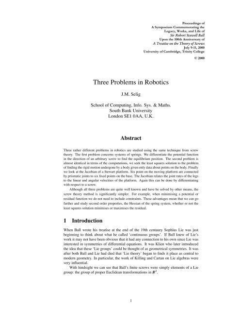
iaiFigure 2: A General Stewart PlatformFor parallel manipulators it is the inverse kinematics that is straightforward, whilethe forward kinematics are hard. Suppose that we are given the position and orientationof the platform the leg-lengths are simple to find. Let us write a i for the position ofthe centre of the spherical joint on the ground belonging to the i-th leg. In the homeconfiguration the corresponding position of the joint centre on the platform will be, b i .So now the length of the i-th leg, or rather its square, can be written,li 2 = ( ) T )ã i − M ˜b i(ãi − M ˜b i i = 1,...,6As usual M is a rigid transformation, this time the motion that takes the platform fromhome to the current position. Notice that the leg-lengths can be thought of as functionson the group, however it is more usual to think of these as components of a mappingfrom the group to the space of leg-lengths, SE(3) −→ IR 6 . A point in IR 6 is given incoordinates as (l 1 , l 2 ,...,l 6 ). It is the jacobian of this mapping that we seek. To do thiswe take the derivative of the leg-lengths,Rearranging this gives,dl 2 idt∣ = 2l i ˙l i = −2 ( ) T ã i − ˜b i S˜b it=0˙l i = 1 l i(˜b i − ã i) T S˜b i = 1 l i((ai × b i ) T ,(b i − a i ) T )( ωvThis gives the joint rate of each leg as a linear function of the velocity screw of theplatform. The jacobian J is the matrix satisfying the formula,⎛⎝⎞ ˙l 1.˙l 6( )⎠ ω= Jv)7

So we see that the rows of this Jacobian matrix are simply,1 ((ai × b i ) T ,(b i − a i ) T ) , i = 1,...,6l iThis is the wrench given by a unit force directed along the i-th leg.Consider a system of springs as in section 2. Suppose there are just six springs.Now it can be shown that the Jacobian associated with the equilibrium position is singular.To see this consider equations (1) and (2), which define the equilibrium position,if we arrange things so that the equilibrium position is the reference position and henceR = I and t = 0 then the equations become,∑λ i a i × b i = 0iand∑λ i (a i − b i )=0iIn term of the Jacobian for a corresponding Stewart platform, that is, one whose leglengthscorrespond to the lengths of the springs, we see that the rows of the Jacobianare linearly dependant and hence the matrix is singular.The forward kinematics problem for a Stewart platform is to determine the positionand orientation of the platform given the leg-lengths. It is well known that, for a givenset of leg-lengths there are a finite number of different solutions, in general 40. Differentsolutions are referred to as different poses or postures of the platform. Replacingthe legs with springs it is clear that the potential function will have the same value ineach of these poses or postures since the function only depends on the lengths of thesprings. However, we can also see that none of these positions will be minima of thepotential function since we know the stable equilibrium position is unique.5 The Stiffness MatrixThe problems presented in the last three sections are well known and have been solvedby many different methods. The advantage of the screw theory methods studied is thatwe can go further and look at higher derivatives.First we note that it is possible to find the wrench due to the springs. In general awrench is a 6-dimensional vector of forces and torques,( )τW =Fwhere τ is a moment about the origin and F is a force. Notice that wrenches are notLie algebra elements but elements of the vector space dual to the Lie algebra. Usuallythe force due to a potential is given by its gradient. The same is true here, in termsof the exterior derivative d we have, W = −dΦ. Pairing the wrench with an arbitraryscrew S gives,W (S)=−dΦ(S)=−∂ S Φsee [13, §. 4.20] for example. Hence we have already done the calculations in section 2above, the wrench is given by,W =( )∑i λ i a i × (a i − Rb i − t)∑ i λ i (a i − Rb i − t)8

this could, of course, also have been deduced from elementary mechanics.For the spring systems of section 2 an important object is the stiffness matrix of thesystem. In this section we show how to compute this by taking the second derivativesof the potential function.An infinitesimal displacement of the body is represented by a screw. The wrenchproduced by a displacement s is given by W = Ks, where K is the stiffness matrix.The stiffness matrix is the hessian of the potential function, that is its matrix ofsecond order partial derivatives, see [1, Ch 5]. This is only valid at an equilibriumposition.There have been attempts in the Robotics literature to extend these ideas to nonequilibriumconfigurations, see for example Griffis and Duffy [4] and Žefran and Kumar[18]. In this work, however, the classical definition of the stiffness matrix will beused.Now let us write the result above for the wrench as( )Ai 0 )W = ∑λ iIi 3 0(ãi − M ˜b iDifferentiating this along an arbitrary screw gives,( )(Ai 0 RBi R∂ S W = ∑λ T )+ T I 3 ωiIi 3 0 0 0)(vusing the result of section 2. Hence, we have that the stiffness matrix is,( )∑i λ i (A i RB i R T + A i T ) ∑ i λ i A iK =∑ i λ i (RB i R T + T ) ∑ i λ i I 3This time we choose the origin to be at the point ∑ i λ i a i and then use the equilibriumcondition 2 to simplify the stiffness matrix to,( )∑i λ i A i RB i R T 0K =0 ∑ i λ i I 3This is a particularly neat result but it is a little surprising at first sight. The term∑ i λ i I 3 in the bottom right corner means that the system has the same stiffness in anydirection, irrespective of the stiffness of the individual springs and their arrangement.This is due to the assumption that the springs have zero natural length.Now we can return to the problem of finding the index of the critical points we havefound. For brevity we will just look at which of the critical points is a minimum of thepotential energy, that is a stable equilibrium. That is: which of the solutions for R givesa stiffness matrix K with all positive eigenvalues? Notice that three of the eigenvaluesof K are simply ∑ i λ i , and this is positive if the spring constants λ i are all positive. Sowe just have to look at the eigenvalues of the top-lefthand bock of K. After a littlemanipulation this can be written in term of the matrix P or its polar decomposition,∑λ i A i RB i R T = RP T + Tr(RP T )I 3 = R i Q + Tr(R i Q)I 3iHere Tr() represents the trace of the matrix. Now this matrix has the same eigenvectorsas R i Q and hence as Q, remember R i was either the identity or a rotation of π about9

an eigenvector of Q. So let us assume that the eigenvalues of Q are µ 1 , µ 2 and µ 3with corresponding eigenvectors e 1 , e 2 and e 3 . Assuming that R i is a rotation abouteigenvector e i , we can find the eigenvalues of the matrices by considering the action onthe eigenvectors e 1 , e 2 and e 3 . The eigenvalues for R 0 Q + Tr(R 0 Q)I 3 are,(2µ 1 + µ 2 + µ 3 ), (µ 1 + 2µ 2 + µ 3 ), and (µ 1 + µ 2 + 2µ 3 )We only need to look at one other matrix since the other are just cyclic permutations,the eigenvalues of R 1 Q + Tr(R 1 Q)I 3 are,(2µ 1 − µ 2 − µ 3 ), (µ 1 − 2µ 2 − µ 3 ), and (µ 1 − µ 2 − 2µ 3 )Now there are just two cases to consider, if det(P) > 0 then we can assume that Qis positive-definite and thus so are all its eigenvalues. In this case it is easy to see thatthe critical point represented by R 0 will be the minimum. This is the solution R = R p .In the other case det(P) < 0, the classical polar decomposition gives us a positivedefinitesymmetric matrix and a reflection. When we multiply these by −1 wegetarotation and a negative-definite symmetric matrix. That is Q has all negative eigenvalues.If we assume that these eigenvalues have the ordering 0 > µ 1 ≥ µ 2 ≥ µ 3 , that is µ 1is the eigenvalue of smallest magnitude, then the matrix, R 1 Q + Tr(R 1 Q)I 3 will haveall positive eigenvalues and hence R 1 corresponds to the minimum of the potential. Soin general, if det(P) < 0 the minimum solution is given by R = R p R i , where R i is arotation of π about the eigenvector of Q with eigenvalue of smallest magnitude.6 ConclusionsThe concept unifying the three problems we have studied in this work is the idea offunctions defined on the group of rigid body transformations. We have been able to findthe stationary points of the functions and classify these critical points. This involves asimple technique of differentiating along a screw.The results agree with those of Kanatani [7, Chap. 5], his methods were, perhaps,a little more elegant than the above. But the methods used here are more general, wehave found all the critical points of the potential function not just the minimum andwith a little more effort we could find the index of each of them.These ideas are central to the subject of Morse theory, a field of study which relatesthe critical points of functions defined on a manifold to the topology of the manifolditself. In this case the topology of the manifold, the underlying manifold of the groupSO(3), is well known, and we can use this to say something about the critical point ofour potential function.The problem of the springs is a slightly artificial one in that we have used springswill zero natural length. This simplifies the computations. It is possible to repeat mostof the above analysis using spring with a finite natural length, see [14]. The numberof critical points now becomes a very hard problem but will still be constrained by thetopology of the group.The problem of estimating a rigid motion from point data is reasonably realistic.The utility of the estimate will depend on the distribution of error for the measuredpoints. There are some results on this in the literature, see [17]. However, I believethere is much scope for further research in this direction.10

We have only had time here to take a brief look at the implications for the Stewartplatform. Certainly using the technique of differentiating along a screw we could workout the acceleration properties of the Stewart platform. However, the usual difficultieson the geometric definition of a second derivative arise here. In particular circumstancesit is clear what should be done, for example it is not too difficult to find thedynamics of a Stewart platform, see [15]. Once again, I believe that the implicationsof the ideas presented here have yet to be fully understood.References[1] V.I. Arnol’d. Geometrical Methods of Classical Mechanics, volume 60 of GraduateTexts in Mathematics. Springer-Verlag, New York, 1978.[2] R.S. Ball. The Theory of Screws. Cambridge University Press, Cambridge, 1900.[3] M. Greenberg. Lectures on Algebrac Topology. W.A. Benjamin Inc., New York,1967.[4] M. Griffis and J. Duffy. Global stiffness modelling of a class of simple compliantcoupling. Mechanism and Machine Theory, 28(2):207–224, 1993.[5] B.K.P Horn. Closed-form solution of absolute orientation using unit quaternions.Journal of the Optical Society of America, A-4:629–642, 1987.[6] R.A. Horn and C.R. Johnson. Matrix Analysis, Cambridge University Press,Cambridge, 1985.[7] K. Kanatani. Geometric Computation for Machine Vision. Clarendon Press, Oxford,1993.[8] J.K. MacKenzie. The estimation of an orientation relationship. Acta. Cryst., 10,pp. 62–62 1957.[9] J. Milnor. Morse Theory. Princeton University Press, New Jersey, 1969.[10] P.A.P. Moran. Quaternions, Harr measure and estimation of paleomagnetic rotation.In J. Gani (ed.), Perspectives in Prob. and Stats., pp. 295–301, AppliedProbability Trust, Sheffield 1975.[11] A. Nádas. Least squares and maximum likelihood estimation of rigid motion.IBM Research report, RC6945, IBM, Yorktown Heights, NY, 1978.[12] W.H. Press, S.A. Teukolsky, W.T. Vetterling and B.P. Flannery. NumericalRecipes in C: the art of Scientific computing 2nd ed. Cambridge University Press,Cambridge, 1992.[13] B.F. Schutz. Geometrical Methods of Mathematical Physics. Cambridge UniversityPress, Cambridge, 1980.[14] J.M. Selig. The Spatial Stiffness Matrix from Simple Stretched Springs In Proceedingsof the 2000 IEEE International Conference on Robotics and Automation,San Fransisco CA, toappear.11

[15] J.M. Selig and P.R McAree. Constrained Robot Dynamics II: Parallel MachinesJournal of Robotic Systems, 16, pp.487–498, 1999.[16] G. Wahba. Section on problems and solutions: A least squares estimate of satelliteattitude. SIAM rev, 8, pp.384–385, 1966.[17] G.S. Watson. Statistics of Rotations, In Lecture Notes in Mathematics, SpringerVerlag, 1379, pp.398-413, 1989.[18] M. Žefran and V. Kumar. Affine connection for the cartesian stiffness matrix.In Proceedings of the 1997 IEEE International Conference on Robotics and Automation,Albuquerque, NM, pages 1376–1381.12