linear vibration analysis using screw theory - helix - Georgia Institute ...

iiiDEDICATIONÀ mon …ls Matthieu

ivACKNOWLEDGMENTSFirst and foremost, I have to thank my family for their encouragement and support during mynumerous years as a graduate student. My parents are largely responsible for this research. Hadthey not stressed the importance of a good education, I never would have attended graduate school.I want to thank the members of my dissertation committee for taking the time to review thisthesis. Particularly, my advisor Dr. Harvey Lipkin for his able direction and for the many hoursspent discussing this research. I also want to thank my o¢cemates, Namik Çiblak and John Alexioufor their suggestions. Also, a special thank to Dr. William Wepfer for his help and encouragements.Finally, I would like to acknowledge the support of the NASA Kennedy Space Center throughtheir Graduate Student Researchers Program.

vi5 FORCED VIBRATIONS : : : : : : : : : : : : : : : : : : : : : : : : : : : : : : : : : : : : : : : : : : : : : : : : : : : : : : : : : : : : : 995.1 Response to Harmonic Excitation . . . . . . . . . . . . . . . . . . . . . . . 995.2 Base Excitation . . . . . . . . . . . . . . . . . . . . . . . . . . . . . . . . . . . 1075.3 Concluding Remarks . . . . . . . . . . . . . . . . . . . . . . . . . . . . . . . 1136 DAMPED VIBRATIONS : : : : : : : : : : : : : : : : : : : : : : : : : : : : : : : : : : : : : : : : : : : : : : : : : : : : : : : : : : : : 1156.1 Planar Motion . . . . . . . . . . . . . . . . . . . . . . . . . . . . . . . . . . . 1176.2 Spatial Motion . . . . . . . . . . . . . . . . . . . . . . . . . . . . . . . . . . . 1426.3 Forced Damped Vibrations . . . . . . . . . . . . . . . . . . . . . . . . . . . . 1496.4 Concluding Remarks . . . . . . . . . . . . . . . . . . . . . . . . . . . . . . . 1577 OTHER RESULTS : : : : : : : : : : : : : : : : : : : : : : : : : : : : : : : : : : : : : : : : : : : : : : : : : : : : : : : : : : : : : : : : : : : 1587.1 Equal Principal Sti¤nesses . . . . . . . . . . . . . . . . . . . . . . . . . . . . 1587.2 Combined Elastic Centers . . . . . . . . . . . . . . . . . . . . . . . . . . . . 1597.3 Decomposition of the Damping Matrix . . . . . . . . . . . . . . . . . . . . 1688 CONCLUSION: : : : : : : : : : : : : : : : : : : : : : : : : : : : : : : : : : : : : : : : : : : : : : : : : : : : : : : : : : : : : : : : : : : : : : : :1738.1 Contributions . . . . . . . . . . . . . . . . . . . . . . . . . . . . . . . . . . . . 1738.2 Further Research . . . . . . . . . . . . . . . . . . . . . . . . . . . . . . . . . . 175APPENDIXA. Proof of Critically Damped Solution . . . . . . . . . . . . . . . . . . . . . . 178REFERENCES : : : : : : : : : : : : : : : : : : : : : : : : : : : : : : : : : : : : : : : : : : : : : : : : : : : : : : : : : : : : : : : : : : : : : : : : : : : 184VITA: : : : : : : : : : : : : : : : : : : : : : : : : : : : : : : : : : : : : : : : : : : : : : : : : : : : : : : : : : : : : : : : : : : : : : : : : : : : : : : : : : : : : : : 187

viiLIST OF FIGURES1.1 Elastically Suspended Rigid Body . . . . . . . . . . . . . . . . . . . . . . . . . . . . . . 21.2 Planar Rigid Body Rotates About V . . . . . . . . . . . . . . . . . . . . . . . . . . . . . 21.3 Body Rotates and Translates about Vibration Axis V . . . . . . . . . . . . . . . . . . . 42.1 Location of the Screw Axes . . . . . . . . . . . . . . . . . . . . . . . . . . . . . . . . . . 82.2 Cantilever Beam . . . . . . . . . . . . . . . . . . . . . . . . . . . . . . . . . . . . . . . . 92.3 Beam Has Three Compliant Axes . . . . . . . . . . . . . . . . . . . . . . . . . . . . . . . 123.1 Elastically Suspended Rigid Body . . . . . . . . . . . . . . . . . . . . . . . . . . . . . . 243.2 Location of Vibration Centers . . . . . . . . . . . . . . . . . . . . . . . . . . . . . . . . . 303.3 Location of Vibration Centers when EM y = 0 . . . . . . . . . . . . . . . . . . . . . . . . 313.4 Location of Vibration Centers when ! 2 x = !2 y . . . . . . . . . . . . . . . . . . . . . . . . 313.5 Perpendiculars intersect at M . . . . . . . . . . . . . . . . . . . . . . . . . . . . . . . . . 333.6 Cantilever Beam . . . . . . . . . . . . . . . . . . . . . . . . . . . . . . . . . . . . . . . . 353.7 Three Vibration Centers . . . . . . . . . . . . . . . . . . . . . . . . . . . . . . . . . . . . 373.8 Two Vibration Centers and One Translation Parallel to the x-axis . . . . . . . . . . . . 373.9 Two Vibration Centers and One Translation Parallel to the y-axis . . . . . . . . . . . . 383.10 Two Vibration Centers and One Translation Parallel to ¡¡! EM . . . . . . . . . . . . . . . 383.11 Trivial Case . . . . . . . . . . . . . . . . . . . . . . . . . . . . . . . . . . . . . . . . . . . 394.1 Elastically Suspended Rigid Body . . . . . . . . . . . . . . . . . . . . . . . . . . . . . . 404.2 Pure Translation Produces Reaction Wrench . . . . . . . . . . . . . . . . . . . . . . . . 424.3 Pure Couple Produces Reaction Twist . . . . . . . . . . . . . . . . . . . . . . . . . . . . 434.4 Robot in Contact with a Compliant Environment . . . . . . . . . . . . . . . . . . . . . . 434.5 Planar Model . . . . . . . . . . . . . . . . . . . . . . . . . . . . . . . . . . . . . . . . . . 614.6 Translation Mode is Present . . . . . . . . . . . . . . . . . . . . . . . . . . . . . . . . . . 654.7 Couple Mode is Present . . . . . . . . . . . . . . . . . . . . . . . . . . . . . . . . . . . . 684.8 Body 2 Designed as Vibration Absorber . . . . . . . . . . . . . . . . . . . . . . . . . . . 694.9 Rigid Body Absorber for a General Wrench . . . . . . . . . . . . . . . . . . . . . . . . . 834.10 Planar Motion with General Wrench . . . . . . . . . . . . . . . . . . . . . . . . . . . . . 864.11 . . . . . . . . . . . . . . . . . . . . . . . . . . . . . . . . . . . . . . . . . . . . . . . . . . 934.12 General Wrench - No Restrictions on M 2 . . . . . . . . . . . . . . . . . . . . . . . . . . 954.13 Possible Design to Suppress Motion due to ~ f . . . . . . . . . . . . . . . . . . . . . . . . 965.1 Location of Forcing Function . . . . . . . . . . . . . . . . . . . . . . . . . . . . . . . . . 1015.2 Mode 3 is Not Excited . . . . . . . . . . . . . . . . . . . . . . . . . . . . . . . . . . . . . 1015.3 Modes 2 and 3 are Not Excited . . . . . . . . . . . . . . . . . . . . . . . . . . . . . . . . 1025.4 Location of Forcing Wrench . . . . . . . . . . . . . . . . . . . . . . . . . . . . . . . . . . 1045.5 Body Excited by the Motion of its Base . . . . . . . . . . . . . . . . . . . . . . . . . . . 1075.6 Mode 1 is not Excited . . . . . . . . . . . . . . . . . . . . . . . . . . . . . . . . . . . . . 1105.7 Mode 1 is not Excited . . . . . . . . . . . . . . . . . . . . . . . . . . . . . . . . . . . . . 1115.8 Mode 1 is not Excited . . . . . . . . . . . . . . . . . . . . . . . . . . . . . . . . . . . . . 112

ixSUMMARYA novel analysis is proposed for the vibration of an elastically suspended rigid body. This newanalysis is based on recent discoveries about the structure of sti¤ness and inertia.For a single planar body, vibration centers are used to describe the modes shapes and areshown to be constrained to regions speci…ed by the center of elasticity, center of mass, and sti¤nessprincipal directions. Responses are classi…ed by the number of pure translation modes and conditionsfor existence are given.Necessary or su¢cient conditions for the existence of pure translation and pure couple modesare also given for spatial articulated and rigid bodies. It is shown that these two types of modes canbe used to design a multi-degree of freedom vibration absorber.For non-proportionally damped planar vibrations of a single rigid body, the modes shapes areshown to be rotations about a point which is either stationary or traveling along a straight linedepending on the type of damping (undamped, underdamped, critically damped, overdamped).Similarly, the spatial mode shapes are rotations and parallel translations about an axis which iseither stationary or traveling along a cylindroid. An explanation of the transition between types ofdamping is also given.Analysis of the forced (damped and undamped) vibrations for planar and spatial motion showshow to avoid exciting a particular mode.Other results include some properties associated with the sti¤ness matrix and a decompositionof the damping matrix based on two singular eigenvalue problems.The research makes signi…cant contributions to understanding the relationship between constitutiveproperties (sti¤ness and inertia) and modal characteristics (natural frequencies and mode

xshapes). Finally, the application of the results to the design of mode shapes and to the inverse modeshape problem are outlined. Numerical examples illustrate the results.

CHAPTER IINTRODUCTIONThe purpose of this research is to investigate the linear vibration problem modelled by a Cartesianset of coordinates. When performing a vibration analysis, one usually needs to solve an eigenvalueproblem. It is essentially a numerical exercise and is di¢cult to interpret. For example,using the eigenvectors to diagonalize the sti¤ness and mass matrices represents a change of basis,but in general this change of basis is neither a rotation nor translation and hence has no obviousphysical meaning. In order to meet speci…cations on the vibrational response of a given system,a designer typically uses trial and error.The goal of this research is to uncover the underlyinggeometrical meaning behind the vibration problem to provide a formulation for a more systematicdesign method.To achieve this goal, the study concentrates on analyzing a single elastically suspended rigidbody (Figure 1.1). The constitutive properties of such a system are modelled by a 6 £ 6 Cartesiansti¤ness matrix K and a 6£6 Cartesian mass matrix M. It is noted that both matrices are symmetricpositive de…nite. The free vibration analysis of this linear system then involves solving an eigenvalueproblem of the form,¡K ¡ ! 2 M ¢ ^T = 0 (1.1)The results are the natural frequencies (! i ) and the 6 £ 1 mode shapes (^T i ). Although the solutionis direct, the relationships between the constitutive properties (K, M) and the modal characteristics(! i , ^T i ) are complex and mostly unknown except in very simple cases. The physical signi…cance ofthese relationships is the focus of this research.Screw Theory, which was developed by Ball[2], is used extensively throughout this thesis. Therelevant parts of this theory are presented in Chapter 2. In addition, Chapter 2 also details some

2Figure 1.1: Elastically Suspended Rigid BodyVEMyzxFigure 1.2: Planar Rigid Body Rotates About Vrecent discoveries about the structure of sti¤ness and inertia which are important to the developmentof the analysis.Patterson and Lipkin[35] and Lipkin[30] proposed a new decomposition of thesti¤ness and inertia matrices each based on two singular eigenvalue problems. The research presentedin this thesis applies these new decompositions to vibration analysis to provide more physical insightinto the vibration eigenvalue problem. Finally, the chapter reviews the relevant work done by otherresearchers.Chapter 3 details the analysis of the planar vibrations of an elastically suspended rigid body.Planar rigid body mode shapes are either a pure translation or a pure rotation about a point in theplane termed a vibration center (V ) (see Figure 1.2) or more commonly a node. The constitutive

3properties have canonical forms: for inertias they are a center of mass, principal directions, and principalvalues of inertia; for sti¤ness they are a center of elasticity, principal directions, and principalvalues of sti¤ness. The modal properties are expressed directly in terms of these quantities usinga Cartesian set of coordinates. This yields several new results that show how the vibration centersmust be con…ned to speci…c regions and develops simple criteria for the existence of translationalmodes.The extension of the previous work to the spatial case is the main focus of Chapter 4. In threedimensional motion, the mode shapes are rotations and parallel translations along an axis in spacetermed vibration axis (V ) (see Figure 1.3).The new decompositions of the sti¤ness and inertiamatrices are used to analyzed the existence of pure translation modes. Unlike the planar case, theconditions for the existence of translation modes are either necessary or su¢cient. A new type ofmode de…ned as couple mode is also introduced. This mode exists when the suspension exerts a purecouple on the body. Similar to pure translation modes, the necessary or su¢cient conditions for theexistence of couple modes are examined. Moreover, it is shown that looking for couple modes isactually the dual problem to looking for translation modes. These analyses are not only conductedfor a single rigid body on an elastic suspension but also for so-called articulated inertias. Articulatedinertias were introduced by Featherstone[20] and are useful in representing the inertia of a chain ofkinematically connected bodies. Finally, it is shown that translation and couple modes can be usedto design a multi-degree of freedom vibration absorber.Chapter 5 presents the analysis of the forced vibrations of a rigid body. For planar motion, itis shown how the location of the vibration centers a¤ects the response of the body to a particularexcitation. For spatial motion, the results are more complicated but an interpretation is still possible.The response of the body does not depend only on the relative position of the excitation and the

4VFigure 1.3: Body Rotates and Translates about Vibration Axis Vvibration axis but also depends on non-geometric quantities. Similar results are obtained for a bodywhich is excited by the motion of its base.The motion of a body undergoing non-proportionally damped vibrations has always been dif-…cult to visualize. Chapter 6 shows that for planar motion, a mode is actually a rotation about apoint which is either stationary or traveling along a straight line depending on the type of damping(undamped, underdamped, critically damped or overdamped). In a similar manner, it is shown thatfor spatial motion, a mode is a screwing motion about a vibration axis which is either stationaryor traveling along a cylindroid. The analysis of forced damped vibrations also yields the conditionsunder which a mode will not respond to an excitation.Other results not directly related to this research are presented in Chapter 7. The …rst twosections detail some properties associated with the sti¤ness matrix. In addition, a decompositionof the damping matrix is presented; this decomposition is based on the same principles that Lipkinand Patterson used to decomposed the sti¤ness and inertia matrices.Finally, Chapter 8 concludes the thesis by summarizing the results and by proposing the applicationof this research to several problems. These include the design of mode shapes, the inverse

5mode shape problem where eigendata is used to reconstruct the sti¤ness and inertia properties of asystem, and also modal identi…cation problems.

CHAPTER IIBACKGROUNDIn this chapter, basic notation and theory are presented as well as the relevant work done byother researchers.2.1 Screw TheoryThe basic concept behind screw theory is to combine linear and rotational motion into oneequation. For example, Hooke’s Law becomes,w O = K O T O (2.1)where K O is the 6 £ 6 sti¤ness matrix and w O and T O are 6 £ 1 entities named wrench and twistrespectively and for small displacements are given by2 3 2~ fw O = 6 74 5 T O = 64~¿ O~ ±O~°375 (2.2)where ~ f, ~¿ O , ~ ± O and ~° are respectively the applied force vector, torque vector, the resulting lineardisplacement vector, and angular displacement (rotation) vector. It is noted that ~° is a genuinevector because only small displacements are considered. The subscript O is introduced to indicatethe origin dependency of the torque and linear displacement vectors as well as the sti¤ness matrix.The resulting equation is then a 6 £ 6 equation. A similar equation can be written for Euler’s Laws,w O = d dt (M OV O ) (2.3)where M O is the 6 £ 6 mass matrix and V O is a velocity twist given byV O =¸ ·~vOÁ ~(2.4)

7where ~v O and ~ Á are respectively the linear velocity and angular velocity vectors. Wrenches andtwists can be written at di¤erent origins and transform according to the following laws,where X OP is de…ned asw P = X T OP w O T P = X ¡1OP T O V P = X ¡1OP V O (2.5)X OP =2641 ¡! OP£0 1375 (2.6)1 is the 3£3 identity matrix, and ¡! OP is the vector from the old origin O to the new origin P. ¡! OP£is the skew symmetric matrix representation of the cross product. The transformation laws (2.5)lead to the following parallel axis congruence transformations for the mass and sti¤ness matrices,M P = X T OP M O X OP K P = X T OP K O X OP (2.7)Ball[2] de…ned the screw-axis of a wrench as the unique line of action in space where the wrenchis equipollent to a force and a parallel torque. A similar de…nition exists for the screw-axis of a twistas the unique rotation axis where the twist is equivalent to a rotation and a parallel translation. Forpoints on the screw-axes, the wrench and twist have the following forms,2 3 2 3~ fh ° ~°w = 6 74 5 T = 6 74 5 (2.8)h f~ f ~°where h f and h ° are scalars de…ned as the pitch of the screw. When w and T are normalizedsuch that ~f ¢~f = 1 and ~° ¢ ~° = 1 then the resulting wrench and twist become screws. Screws are towrenches and twists what unit vectors are to vectors. The transformation laws (2.5) are used to …ndthe location of the screw-axis of a given wrench or twist (see Figure 2.1).2.2 Decomposition of the Sti¤ness MatrixLipkin and Patterson[35] proposed a new decomposition for the sti¤ness matrix. Their decompositionis based on the solutions to two eigenvalue problems referred to as the eigenwrench problem

8τ OOfδ OORWrenchScrew−AxisOOFfh f fγTwistScrew−Axish γγγFigure 2.1: Location of the Screw Axesand the eigentwist problem.Consider a rigid body on an elastic suspension like the one shownin Figure 1.1. The eigenwrench problem is stated as, what wrenches (w f ) can be applied to thebody so that the resulting twists are pure translations parallel to the wrenches? The eigentwistproblem is stated as, what twists (T ° ) can be applied to the body so that the resulting wrenches arepure torques parallel to the rotation? Mathematically, the eigenwrench problem and the eigentwistproblem are respectively,k f w f = K¡w f k ° ³T ° = KT ° (2.9)where k f and k ° are the eigenvalues of each problem and2 3 21 0¡ = 640 075 ³ =640 00 1375 (2.10)Although (2.9) represents two 6 £ 1 equations, the solutions to (2.9) are three eigenwrenches w fiand three eigentwists T °i . This result is due to the form of (2.10). Like any eigenvalue problem,the eigenvectors of (2.9) can be normalized. The chosen normalization makes the eigenwrenches andeigentwists screws as de…ned in the previous section (i.e. w fi ¡w fi = 1, T °i ³T ° i= 1). Lipkin andPatterson then showed that the sti¤ness matrix could be decomposed as,2 3· ¸~k f 0· ¸TK = ~w f ~w6 7° 4 5 ~w f ~w °0 ~k °(2.11)

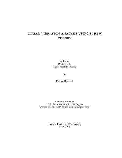
9yOA, I x , I y , Y, LMxm, m γFigure 2.2: Cantilever Beamwhere ~ k f = diag(k fi ) and k ~ ° = diag(k °i ) are 3 £ 3 diagonal matrices representing respectively the·¸stationary values of linear and rotational sti¤nesses. Also ~w f = w f1 w f2 w f3are the three·¸eigenwrenches and ~w ° = w ° 1w °2 w °where w °i = k °i ³T3° iare the reaction torques duethe eigentwists T °i .Finally, the location of each eigenwrench and eigentwist in space is de…ned as the location of itsscrew-axis and can be found by using (2.5), so that each eigenwrench and eigentwist has the form of(2.8). Lipkin and Patterson also found that in general, the axes of the eigenwrenches are orthogonalbut non-intersecting. Similar results were obtained for the eigentwists. They also showed that theeigenwrenches and eigentwists form reciprocal three-systems, i.e.·T °1 T °2 T ° 3¸T ·w f1 w f2 w f3¸= 0 (2.12)The following example illustrates the procedure to …nd the eigenwrenches and eigentwists.2.2.1 ExampleA massless cantilever beam supporting a rigid body (Figure 2.2) is used to illustrate the procedure.The rigid body has its center of mass at the free end of the beam with its principal inertiaaxes parallel to the coordinate system shown in the …gure.The example is only concerned with the motion of the rigid body and hence the elastic beamcan be modeled by a sti¤ness matrix at the free end with shear e¤ects neglected. The sti¤ness is

10then,whereK M =2643K 11 K 1275 (2.13)K T 12 K 2223AY L 2 0 0K 11 = 1 L 3 0 12Y I z 067450 0 12Y I y230 0 0K 12 = 1 L 2 0 0 ¡6Y I z67450 6Y I y 023GJ 0 0K 22 = 1 L0 4Y I y 067450 0 4Y I zwhere A, L, Y and G are respectively the cross-sectional area, the length of the beam, the Young’smodulus and the shear modulus. J is the polar area moment of inertia about the x-axis. I y , I z arethe area moments of inertia about the y and z-axis respectively.First, one must solve for the eigenwrenches w and eigentwists T of the sti¤ness matrix. Solvingthe eigenvalue problems (2.9) yields,23·~w M =¸ w 1 w 2 w 3=641 0 00 1 00 0 10 0 00 0 L=20 ¡L=2 075(2.14)

1123·~T M =¸ T 1 T 2 T 3=640 0 00 0 L=20 ¡L=2 01 0 00 1 00 0 175(2.15)where the subscript M indicates that the eigenwrenches and eigentwists are expressed at point M.The eigenvalue problem also yields,·~k f = diag·~k ° = diagAYLGJL12Y I zL 3Y I zL12Y I yL 3Y I yL¸¸(2.16)(2.17)A simpler expression for the eigenwrenches and eigentwists can be had by using a rigid body translation(2.5) and expressing them at the midpoint of the beam (E),2 3 2 3~w E =641075~T E =640175 (2.18)where 1 is the 3 £ 3 identity matrix. Comparing (2.2) and (2.18) reveals that the eigenwrenchesare all pure forces and intersect at the mid-point of the beam. Furthermore, the eigentwists areall pure rotations, they also intersect at the mid-point of the beam and they are collinear with theeigenwrenches. When a pure force eigenwrench is collinear with a pure rotation eigentwist, it isde…ned as a compliant axis. Hence a cantilever beam has three compliant axes as shown in Figure2.3.

13·where T ° =~ ±T°¸Twas used. Note that ~ ± is a 2£1 vector representing an in plane translationand ° is a scalar representing a rotation perpendicular to the plane. The right equation in (2.23) isa scalar eigenvalue equation with eigenvalue k °i and “eigenvector” ° i normalized so ° i ¢° i = 1. (Theindex i = 1 is retained for symmetry with the spatial case.) Backsubstituting into the left equation· ¸TTin (2.23) yields the single unit eigentwist T ° i= ~ ± i ° i, i = 1. (Note that since ° i = 1, thenthe unit eigentwist no longer represents a “small” deformation but represents a purely geometricquantity, namely an axis of rotation). Furthermore, since the right equation in (2.23) is a scalarequation then the eigenvalue is simply,k °i = C ¡ B T A ¡1 B, i = 1 (2.24)For a spatial sti¤ness, it was shown that the eigenwrenches are reciprocal to the eigentwists (2.12).By using (2.20) and (2.23), it is easily shown that this condition holds for a planar sti¤ness. Hence,the two eigenwrenches are reciprocal to the single eigentwist,T T ° 1w fi = 0 i = 1; 2 (2.25)Finally, the matrix can be decomposed using (2.11) as,K = PK E P T (2.26)where2P = 643~ f1 ~ f2 ~0·75 K E = diag¿ 1 ¿ 2 ° 1k f1 k f2 k ° 1¸(2.27)Obviously, pre-multiplying (2.26) by P ¡1 and post-multiplying by P ¡Tyields a diagonal sti¤nessmatrix as,K E = P ¡1 KP ¡T (2.28)The matrix P is a congruence transformation which represents a change of coordinates. For the

14twist it induces the form T E = P T T where P T is factored as,2 3 2 3· ¸Twhere R = ~ f1 ~ f2·and ¿ =R 01 ¿P T = 6 7 64 5 40 1 0 175 (2.29)¿ 1 ¿ 2¸T. Since ~ f 1 and ~ f 2 are orthogonal (see (2.21)), the …rstmatrix in (2.29) is simply a rotation matrix about an axis perpendicular to the plane. It rotates thecoordinate system to make it parallel to the principal sti¤ness directions.For the second matrix, consider a vector ¡! ·¸TOE= OE x OE y; the planar form of the crossproduct operator is introduced as another vector ¡! ·¸TOE £ = OE y ¡OE x. Since there alwaysexists some ¡! OE such that ¿ = ¡! OE£ then (2.29) becomes2 3 26 R 0 7 6 1 ¡! OE£P T = 6 7 64 5 40 1 0 1and the second matrix is identi…ed as a translation of the coordinate origin from point O to pointE (similar to (2.5)). This special point E always exists in the plane and is termed the center ofelasticity (the next section gives a more general de…nition). The results are summarized by thefollowing theorem,375Theorem 1 The planar sti¤ness matrix can always be diagonalized by a rigid body coordinate transformationcomposed of a translation of the origin to the center-of-elasticity followed by a rotationabout the center-of-elasticity to the principal directions.Moreover, the congruence transformation induces for a wrench w E = P ¡1 w. By using thistransformation, it is easily shown that the eigenwrenches become,2 3·¸ 1w f1 w f2= 6 74 50(2.30)Hence, the following theorem can be stated.

15Theorem 2 For a planar sti¤ness, the eigenwrenches are orthogonal pure forces through the centerof elasticity. Further, the eigenwrenches indicate the principal sti¤ness directions. Moreover, thesingle eigentwist is a pure rotation about the center of elasticity.2.3 Centers of Elasticity, Sti¤ness and ComplianceThe center of elasticity (E) associated with a sti¤ness matrix has been de…ned for specialinstances by a few authors, for special instances [18], [34], and in the most general case [9], [36].Lipkin and Patterson[36], proved that the sum of the three perpendicular vectors from the center ofelasticity to the eigenwrenches or eigentwists is zero. That is3X~r E f i= 0i=13X~r E ° i= 0 (2.31)i=1where ~r E f and ~rE ° are respectively the perpendicular vectors from the center of elasticity to theeigenwrenches and eigentwists. Equation (2.31) shows that each set of vectors are coplanar at E.Consider the following 3 £ 3 partitions of a general 6 £ 6 sti¤ness matrix,2 3K = 64AB TBD75 (2.32)Loncaric[31] proved that by using the congruence transformation (2.7), the o¤-diagonal block (B)will be symmetric at a generally unique point in space. He de…ned that unique point as the centerof sti¤ness (S). He also proved that a similar point exists for the compliance matrix (C = K ¡1 )and termed it center of compliance (C).In general, the centers of sti¤ness and compliance donot coincide. Ciblak and Lipkin[9] were able to show that the location of the centers of sti¤nessand compliance are related to the location of the eigenwrenches and eigentwists by the followingequations,3Xk fi ~r S f i= 0i=13Xi=1k ¡1° i~r C ° i= 0 (2.33)

where ~r S f and ~rC °are respectively the perpendicular vectors from the center of sti¤ness to the eigenwrenchesand from the center of compliance to the eigentwists. Equation (2.33) shows that each setof vectors are coplanar respectively at S and C.The location of the centers of elasticity, sti¤ness and compliance are important parametersa¤ecting the modal response of an elastically suspended rigid body. For planar motion, the threecenters coalesce into a unique point on the plane and as shown above, the sti¤ness matrix becomesdiagonal when expressed at this point. The diagonal elements of the sti¤ness matrix are then the16principal sti¤nesses similar to the principal inertias for the mass matrix.This unique point isalso referred to as the point where there is no dynamic coupling in the equation of motion[43]. Indistinction to the planar case, the spatial 6 £ 6 sti¤ness matrix cannot be generally diagonalized bya rigid body transformation[31]. Although, in some cases like the beam example presented above,the sti¤ness matrix is diagonal at the center of elasticity which in this example is at the midpointof the beam.2.4 Decomposition of the Mass MatrixThe mass matrix can be used to model the inertia of more than one rigid body. For example, itcan be used to model so-called articulated inertias (see [20]) in which case, the mass matrix becomesa full symmetric 6 £ 6 matrix with 21 independent parameters. Articulated inertias are very usefulin analyzing the dynamics of a robot.Lipkin[30] proposed a decomposition for the mass matrix which is similar to the one proposedfor the sti¤ness matrix. His decomposition is also based on two eigenvalue problems. Consideringonly the inertial response of the body shown in Figure 1.1 which is initially at rest, the eigenwrenchproblem becomes, what wrenches (u f ) can be applied to the body so that the resulting accelerationtwists are pure translational accelerations parallel to the wrenches? The eigentwist problem is stated

17as, what acceleration twists (A ° ) can be applied to the body so that the resulting wrenches are purecouples parallel to the twists? Using the usual linear assumptions, the mathematical representationsof the eigenwrench and eigentwist problems are respectively,m f u f = M¡u f m ° ³A ° = MA ° (2.34)where ¡ and ³ are given by (2.10) andu f =264~ f~¿3275 A ° = 64~a~®375 (2.35)are respectively an eigenwrench and eigentwist of the mass matrix. ~a and ~® are respectively thetranslational and angular acceleration. Solving the eigenvalues (2.34) will also yields three eigenwrenchesu i with their associated eigenvalue m fiand three eigentwists A i with their associatedeigenvalue m °i . Once again the eigenwrenches and eigentwists are orthogonal but non-intersectingand can be used to diagonalize the mass matrix as,2 30 ~m °· ¸~m f 0·M = ~u f ~u6 7° 4 5~u f ~u °¸T(2.36)where ~m f = diag(m fi ) and ~m ° = diag(m ° i) are 3 £ 3 diagonal matrices representing respectively·¸the stationary values of linear and rotational (inertia) mass. Also ~u f = u f1 u f2 u f3are the·¸three eigenwrenches and ~u ° = u °1 u °2 u °where ~u ° = ³ ~A3° ~m ° are the reaction torques due·¸the eigentwists. ~A ° = A ° 1A ° 2A °3are the three eigentwists.Similar to the results for the sti¤ness matrix, the eigenwrenches as well as the eigentwists are ingeneral orthogonal but non-intersecting. Further, the eigenwrenches and eigentwists form reciprocalthree-systems.2.4.1 Rigid Body InertiaNote that when this decomposition (2.36) is applied to the inertia of a single rigid body, it isequivalent to …nding the center of mass and the principal inertia directions. The three eigenvalues

18m fi are all equal and represent the mass of the body and the other three eigenvalues m °i are theprincipal inertias. If the mass matrix is expressed at the center of mass and the coordinate systemis parallel to the principal inertias then the eigentwist and eigenwrench problem (2.34) yield thefollowing eigenwrenches and eigentwists,2~u f =6410375~A ° =26401375 (2.37)where 1 is the 3 £ 3 identity matrix and 0 is a 3 £ 3 matrix of zeros.Equation (2.37) reveals that the eigenwrenches are all pure forces through the center of massand that the eigentwists are all pure rotations about the center of mass. Note that the upper blockof ~u f is always equal to 1 regardless of the coordinate system. This property is due to the fact thatthe linear mass of the body is the same in all directions (i.e. ~m f = m1). Hence, any pure forcethrough the center of mass is an eigenwrench of the mass matrix.Unlike the linear mass, the rotational mass (inertia) is in general not equal in all directions(i.e. ~m ° 6= m ° 1) which results in the lower part of ~A ° being equal to 1 only when the coordinatesystem is parallel to the principal inertia directions. Hence, the eigentwists are pure rotations aboutthe center of mass parallel to the principal inertia directions. The results are summarized in thefollowing Theorem.Theorem 3 For rigid body inertia, the eigenwrenches are any pure force through the center of mass.Further, the eigentwists are pure rotations about the center of mass and indicate principal rotationalmass (inertia) directions.

192.4.2 Planar InertiaSimilar to planar sti¤ness, a general planar mass matrix can always be diagonalized by a rigidbody transformation. At the center of mass, the matrix has the following form,23m x 0 0M =0 m y 067450 0 m °(2.38)Note that for a general inertia (as opposed to rigid body inertia), m x 6= m y . Since the mass matrixexhibits the same properties as the sti¤ness matrix, the following theorem holds (see Theorem 2).Theorem 4 For general planar inertia, the eigenwrenches are orthogonal pure forces through thecenter of mass. Further, the eigenwrenches indicate the principal linear mass directions. Moreover,the single eigentwist is a pure rotation about the center of mass.Obviously, if a single rigid body is considered then m x = m y and similar to the spatial case,the eigenwrenches now become any pure force through the center of mass which yields the followingtheorem.Theorem 5 For planar rigid body inertia, the eigenwrenches are any pure forces through the centerof mass.2.5 Eigenwrench and Eigentwist SpaceThe eigenwrenches are the basis elements of the eigenwrench space which is de…ned as the linearcombination of the three eigenwrenches and is denoted S w . Similarly, the eigentwists are the basiselements of the eigentwist space which is de…ned as the linear combination of the three eigentwistsand is denoted S T . Each space only contains a portion of all possible wrenches or twists (six linearlyindependent wrenches or twists are required to described all wrenches and twists). The wrenchesand twists contained in those spaces have a very important property which is addressed below.

20Consider any wrench contained in the eigenwrench space of the sti¤ness matrix (Sw K ), that is,w 2S K w (2.39)then the wrench can be represented by a linear combination of the eigenwrenches,½where w fi 2 Bw K and Bw K =3Xw = ¸iw fi (2.40)i=1¾w f1 w f2 w f3is the set of eigenwrenches of the sti¤ness matrix.The resulting twist is T = K ¡1 w. Since the w fi satis…es (2.9), one can substitute (2.9) to yield,3332~ f1f 1T =¸1k ¡1 64~02~ f2f 27 ¡15 + ¸2k 64~02~ f3f 37 ¡15 + ¸3k 64~075 (2.41)where w fi =· ¸~ fi ~¿ iwas used.Equation (2.41) shows that the resulting twist T is a puretranslation and since the ~ f i are linearly independent, it means that any pure translation is due to awrench contained in the eigenwrench space of the sti¤ness matrix. By following the same procedurefor the eigentwists, one can prove that any pure couple is due to a twist contained in the eigentwistspace of the sti¤ness matrix. Those results also hold for the eigenwrenches and eigentwists of themass matrix.2.6 Literature SurveyThe most relevant work done on the structure of sti¤ness and inertia was presented in theprevious sections. Very little work has been done on combining screw theory with vibration analysis.In analyzing the free vibrations of an elastically suspended rigid body, Ball[2] was the …rst to realizethat the mode shapes were actually screws which he termed harmonic screws. That is a mode shapecan be represented by a translation and parallel rotation along an axis. As noted in Chapter 1, Ball’sharmonic screws are referred to as vibration axes in this thesis. Ball did setup the problem using

21screws but never analyzed it except for special cases where the motion of the body was constrained.Dimentberg[18] did consider the problem but gave very few speci…c results. His only result was thatthe equations of motion are decoupled when the sti¤ness matrix is diagonal and when the principalsti¤ness directions are parallel to the principal inertia directions. Essentially, he only solved the casewhere both the sti¤ness and mass matrix are diagonal.Crede and Harris[15] analyzed the vibrations of a rigid body supported by line springs parallelto the principal inertia axes. Although they solved the problem using the usual eigenvalue problem,they noticed that some modes decouple when the sti¤ness distribution has one, two, or three planesof symmetry with respect to the center of mass. If the system has one plane of symmetry then thesolution can be split into two problems, one for in-plane motion and one for out-of-plane motion eachcontaining three modes. When two planes of symmetry exist then the modes are one translationand one rotation along the intersection of the two planes (the z-axis for example) and four othermodes, two in each plane. These four modes are coupled: x-axis translation and y-axis rotation forthe x-z plane and vice-versa for the y-z plane. Finally, for three planes of symmetry, all modes aredecoupled. Crede and Harris also proved that for any orientation of the line springs, the necessaryconditions for total decoupling are that any pure translation of the body produces a resultant elasticforce through the center of mass and that any torque applied to the body results in a rotation aboutan axis through the center of mass. Their analysis is interesting but lacks generality since it is limitedto line springs. Moreover, they are only concerned with decoupling the modes and hence do notprovide any information when the modes are coupled. Furthermore, Crede[14] also considered thecase where two symmetry planes exist and one principal inertia axis is collinear with the intersectionof the two planes; the other two principal inertia axes directions are arbitrary. He found that onlyone mode decouples, namely a translation parallel to the intersection of the two planes.As mentioned earlier, the design of vibration absorbers is a good application. The literature

22on the subject is extensive [15], [19], [23], [24], [29], [41], [42], [43] to name a few. In general theresearchers have focused on designing single degree of freedom vibration absorbers. The new analysispresented in this thesis is useful for designing multi-degree of freedom absorbers. These multi-degreeof freedom absorbers are more versatile than usual absorber.Vibration analysis is usually performed to ensure that the natural frequencies of the lower modesdo not fall in a speci…ed range. Hence, a number of techniques exist to …nd those modes [15], [33],[43]. Furthermore, the mode shapes are often used to model the response of a system in the socalledassumed modes method[33]. Moreover, several researchers use the mode shapes to decouplethe equation of motion, for example De Schutter and Torfs[17] use the mode shapes to decouple theequation of motion of the end e¤ector of a robot. Decoupling the equations transforms the problemfrom a multi-degree of freedom problem to multiple single degree of freedom problems which areeasier to analyze.Although the mode shapes are used a lot as noted above, their design has largely been ignored.Designing a mode shape has application where the performance of a device relies on a particularmode shape[26]. A few researchers [21], [26], [39] have addressed the design of a mode shape for abeam modeled by lumped-mass or …nite elements.

CHAPTER IIIPLANAR MOTIONThis chapter details the analysis of the planar vibrations of an elastically suspended rigid body.As described in the introduction the analysis makes use of the vibration center concept about whichthe body rotates.The remainder of the chapter is organized as follows. The vibration center locations are formulatedas roots of polynomial equations. The existence of in…nitely distant vibration centers, i.e.translations, leads to a systematic classi…cation of modal responses. The results are geometricallyinterpreted which leads to several elegant and simple relations between the vibration centers andthe canonical constitutive properties. A numerical example illustrates the results.3.1 Equation of MotionV isFor the rigid body in Figure 3.1, the 3 £ 1 equation of motion written at some arbitrary pointM V::TV +K V T V = w V (3.1)where M V is the 3 £ 3 planar inertia matrix, K V is the 3 £ 3 planar sti¤ness matrix, w V is a 3 £ 1planar applied wrench, and T Vis a 3 £ 1 planar deformation twist, all expressed at V . Note thatboth M V and K V are symmetric positive de…nite matrices. w V is composed of a force in the x ¡ yplane and a torque in the z¡direction. Similarly T Vis composed of a small linear deformation inthe x¡y plane and a small angular deformation in the z¡direction. It should be noted that a planarwrench is most generally a planar force along a line of action, and a planar twist is a rotation aboutan axis normal to the plane. The exceptions are when the wrench is a pure torque and the twist apure translation.

24VEMyzxFigure 3.1: Elastically Suspended Rigid BodyBy choosing the coordinate frame direction along the principal sti¤ness directions then theparallel axis congruence transformations (2.7) yield,M V = X T MV M M X MV K V = X T EV K E X EV (3.2)23 23m x 0 0k x 0 0M M =0 m y 0K E =0 k y 0(3.3)67 6745 450 0 m ° 0 0 k °where M M is the inertia matrix at the center of mass (M) and for the planar case is independentof the coordinate directions, m x = m y is the mass, and m ° is the rotational inertia; K E is thesti¤ness matrix at the center of elasticity (E) and is diagonal as discussed in Section 2.2, k x andk y are the linear sti¤nesses in the x and y direction respectively and k ° is the rotational sti¤ness.X MV and X EV are translational transformations (2.6) from the M to V and E to V respectivelyin 3 £ 3 form. It is possible to have m x 6= m y but this requires more than a single rigid bodyand the introduction of kinematic constraints between the bodies. This is sometimes referred to asarticulated or compound inertias [20], [30]. Even though this analysis is only concerned with a singlerigid body, the distinction between m x and m y is retained for generality and greater symmetry.

253.2 Vibration CentersThe eigenvalue problem associated with (3.1) yields three eigenvalues (! 2 ) and three eigenvectors(^T V ). Note that the eigenvectors (^T V ) unlike the motion of the body (T V ), are time independentwhich is emphasized by the use of the hat (^) symbol. Each eigenvector represents either a rotationabout a …nite point V called the vibration center (see Figure 3.1) or a pure translation wherethe vibration center is in…nitely distant.To gain physical insight, it is possible to analyze thecoe¢cients of the cubic in ! 2 . However, these are rather complicated and physical interpretationsare not obvious. An alternative formulation expresses the cubic in terms of a component of ¡¡! MV, thevector from the center of mass to a vibration center. This yields a form that is easier to interpret.To simplify the formulation the two distinct mode shapes are considered in turn, rotations andtranslations.3.2.1 Rotation ModesAssuming …rst that the mode shape is a rotation, then about the vibration center V it has theform,^T V =¸ ·~01(3.4)Next, choosing a coordinate system at V parallel to the principal sti¤ness directions and using (3.2)in the eigenvalue problem of (3.1) yields,¡XTEV K E X EV ¡ ! 2 X T MV M M X MV¢ ^T V = 0 (3.5)Introducing (3.3) and (3.4), ¡! EV = ¡¡! EM + ¡¡! MV, and vector components yields three scalar equationsin the three unknowns ! 2 , MV x , and MV y ,! 2 = ! 2 EV yx = ! 2 MV y + EM yx(3.6)MV y MV y! 2 = ! 2 EV xy = ! 2 MV x + EM xy(3.7)MV x MV x

26! 2 =k ° + k x EVy 2 + k y EVx2m ° + m x MVy 2 + m y MVx2= k ° + k x (MV y + EM y ) 2 + k y (MV x + EM x ) 2m ° + m x MV 2 y + m y MV 2 x(3.8)where for brevity,! 2 x = k xm x! 2 y = k ym y(3.9)From (3.8), the numerator and denominator result from the parallel axis theorem applied to theprincipal rotational sti¤ness and the principal rotational inertia. This leads to the following result,Theorem 6 For a rotation mode shape, the natural frequency squared is the ratio of the e¤ectiverotational sti¤ness to the e¤ective rotational inertia about the corresponding vibration center.To determine a cubic, ! 2 is eliminated from (3.6) and (3.7) to yield the bilinear relation,MV y =! 2 xMV x EM y! 2 y(EM x + MV x ) ¡ ! 2 xMV x(3.10)Eliminating ! 2 from (3.6) and (3.8) and then MV y using (3.10) gives the cubic in the x componentMV x ,[k y (! 2 x ¡ ! 2 y)EM x ]MV 3 x ¡ [! 2 y(k y EM 2 x + k x EM 2 y )¡(! 2 x ¡ ! 2 y)(k y EM 2 x + k ° ¡ ! 2 ym ° )]MV 2x + [! 2 yEM x ((m ° ! 2 y ¡ k ° )¡ (3.11)(k y EM 2 x + k x EM 2 y ) ¡ m ° (! 2 x ¡ ! 2 y))]MV x + ! 4 ym ° EM 2 x = 0It is also useful to rearrange the bilinear equation for MV x and determine the cubic in MV y to givethe complementary relations,MV x =! 2 y MV yEM x! 2 x(EM y + MV y ) ¡ ! 2 yMV y(3.12)[k x (! 2 y ¡ ! 2 x)EM y ]MV 3y ¡ [! 2 x(k x EM 2 y + k y EM 2 x)¡

(! 2 y ¡ !2 x )(k xEM 2 y + k ° ¡ ! 2 x m °)]MV 2y + [!2 x EM y((m ° ! 2 x ¡ k °)¡ (3.13)(k x EM 2 y + k yEM 2 x ) ¡ m °(! 2 y ¡ !2 x ))]MV y + ! 4 x m °EM 2 y = 027The lead coe¢cient of a polynomial vanishes if and only if a root is at in…nity. For the cubicsthis means that one of the components of ¡¡! MV is in…nite and thus the vibration center V is atin…nity since the center of mass is always at a …nite location. However, when the vibration center isat in…nity this indicates a translation mode shape. Since a nonsingular sti¤ness is assumed, thereare three possible conditions that make the lead coe¢cient vanish and thus generate a translationmode,EM x = 0, EM y = 0, or ! 2 x = ! 2 y (3.14)Since the coordinate axes were selected along the principal sti¤ness directions, the …rst twoconditions are equivalent to the center of mass lying on a principal sti¤ness axis .For the lastcondition, since m x = m y then k x = k y so that every line through E is a principal sti¤ness axis andthus one passes through M. Hence the following has been demonstrated,Theorem 7 A translation mode exists if and only if the center of mass lies on a principal axis ofsti¤ness.3.2.2 Translation ModesSecond, consider the eigenvectors to be pure translations. The coordinate directions are againparallel to the principal sti¤ness axes but this time the equations are expressed at the center of massM,¡ ¢XTEM K E X EM ¡ ! 2 M M ^T M = 0 (3.15)

28·where ^T M =~ ±T0¸Tis a translation. Introducing components yields an eigenvalue problemand a constraint equation, 2643! 2 x ¡ ! 2 0·±x75= 0 (3.16)0 ! 2 y ¡ ! 2 ± y¸k x EM y ± x ¡ k y EM x ± y = 0 (3.17)To a scalar multiple, the constraint equation speci…es the translational direction as,2~ ± = 643k y EM x75 (3.18)k x EM y3.2.3 Classi…cation of Modal ResponsesThe di¤erent types of modal responses can be categorized by the number of independent translationmode shapes: zero, one or two. The instance of one translation mode is divided into twosubcases. Each of the cases is illustrated by a …gure whose numerical results are presented in afollowing section.1. Zero translation modes. ! 2 x 6= ! 2 y, and M does not lie on a principal axis of sti¤ness (EM x 6=0; EM y 6= 0) (see Figure 3.7, where V 1 and V 2 are near but not on the x-axis). There are threerotation modes whose centers are given by the cubic and bilinear equations ((3.11), (3.10) or(3.13), (3.12)). The natural frequencies are determined from any of (3.6)-(3.8).2a. One translation mode. M lies on a principal axis of sti¤ness but is not coincident with E(EM x 6= 0, EM y = 0 in Figure 3.8 or EM x = 0, EM y 6= 0 in Figure 3.9 ). Consider only the…rst condition where EM y = 0 since the other is similar. The cubic (3.11) yields MV y = 0,0, 1 indicating that the two …nite vibration centers are on the x principal sti¤ness axis. It isnot possible to determine the x coordinate from either bilinear expression since they becomeindeterminate. Instead, eliminating ! 2 from (3.7) and (3.8) gives the x coordinates as the

29roots of a quadratic equation,(k y EM x )MV 2x + (k ° ¡ m ° ! 2 y + k yEM 2 x )MV x ¡ m ° ! 2 y EM x = 0 (3.19)The corresponding natural frequencies are obtained from (3.7) or (3.8).·The translation mode (3.18) is in the direction of the x principal sti¤ness axis, ~ ± =1 0¸Tand the natural frequency (3.16) is given by ! 2 = ! 2 x. In summary, M and the two …nitevibration centers are on a principal sti¤ness axis and the translation mode is parallel to it.2b. One translation mode. ! 2 x = ! 2 y and although every line through E is a principal axis ofsti¤ness, the chosen x or y principal axes do not go through M (EM x 6= 0, EM y 6= 0) (seeFigure 3.10).The cubic (3.11) for MV x yields one root at in…nity and two nonzero …nitevalues. The two …nite y coordinates (3.10) are also nonzero,MV y = MV xEM yEM x(3.20)This also indicates that ¡¡! EM and ¡¡! MV are parallel so E, M, and the two vibration centers areall collinear. The natural frequencies follow from any of (3.6)-(3.8).The translation mode (3.18) is also in this direction, ~ ± = ¡¡! EM with ! 2 = ! 2 x = ! 2 y. This issimilar to case 2a since the …nite vibrations centers are on a principal sti¤ness axis and thetranslation mode is parallel to it.3. E and M coincide (EM x = 0, EM y = 0) (see Figure 3.11). This is the trivial case when bothK and M are diagonal. One mode is a pure rotation about E and its natural frequency is! 2 = (k ° =m ° ). The two other modes are pure translations parallel to the principal sti¤nessaxes with natural frequencies of ! x and ! y . When ! x = ! y the principal sti¤ness axes andthe parallel translations are in all direction.The cases 2 and 3 containing translation modes are summarized by the following,

30yVMExFigure 3.2: Location of Vibration CentersTheorem 8 Translation modes are parallel to a principal sti¤ness axis with respective natural frequenciesof ! x and ! y .Theorem 9 For one translation mode, the two …nite vibration centers lie on the parallel principalsti¤ness axis. For two translation modes, the one …nite vibration center lies on both principal sti¤nessaxes, i.e. at the center of elasticity E.3.3 Geometric Interpretation3.3.1 Location of Vibration CentersFor a given system, the potential vibration center locations are not arbitrary but con…ned todistinct regions. The preceding analysis is used to identify these regions that can be speci…ed verysimply in terms of the center of mass, the center of elasticity, and the principal sti¤ness directions.Again the three basic cases are considered.Case 1, three distinct centers. Examining (3.6) and (3.7) shows that EV y and MV y must eitherbe both positive or negative and the same for EV x and MV x . The result is that the vibration centerscan only lie in the shaded portion of Figure 3.2.Case 2a, EM y = 0 (or EM x = 0). The two …nite vibration centers lie on the x-axis (y-axis).However from (3.7) ((3.6)) they cannot lie between E and M. Their location MV x is given by the

31yVEMVxFigure 3.3: Location of Vibration Centers when EM y = 0yMVVExFigure 3.4: Location of Vibration Centers when ! 2 x = !2 yroots of (3.19). Since the constant term is negative, the two roots have opposite signs and thereforelie on opposite sides of M. Thus, one vibration center must lie on each side of ¡¡! EM (see Figure 3.3).Case 2b, ! 2 x = ! 2 y and the chosen coordinate system does not go through M. The vibrationcenters are on the line that connects E and M but (3.6) and (3.7) show that they cannot be betweenE and M. Their location MV x is given by (3.11) which reduces to,(k y EM 2 x + k xEM 2 y )MV 2 x ¡ EM x(m ° ! 2 x ¡ k ° ¡ k y EM 2 x ¡ k xEM 2 y )MV x ¡ ! 2 y m °EM 2 x = 0 (3.21)Since the constant term is negative, the two roots have opposite signs and therefore lie on oppositesides of M. Thus, one vibration center must lie on each side of ¡¡! EM (see Figure 3.4). It should benoted that Figures 3.3 and 3.4 are special cases of Figure 3.2.Case 3, E and M are coincident. This is the trivial case and the single …nite vibration centeris also coincident.The results are summarized by the following theorems.

32Theorem 10 When the center of mass does not lie on an axis of principal sti¤ness, then the threevibration centers must lie in the shaded area of Figure 3.2Theorem 11 When the center of mass lies on a principal sti¤ness axis, then the two …nite vibrationcenters also lie on that axis, one on each side of the centers-of-elasticity and mass.3.3.2 Orthogonality ConditionsThe orthogonality conditions also provide geometric constraints on the location of the vibrationcenters. Consider the orthogonality conditions for the mass matrix associated with the eigenvalueproblem written at the center of mass.³^T T M´i M M³^T M´j= 0 i 6= j i; j = 1; 2; 3 (3.22)where³^T M´= (X MV ) i ^T V and i, j denote the mode number. Rewriting (3.22) for modes i, ki(k 6= j) and subtracting from (3.22) results in,¡¡!MV i ¢ V ¡¡¡!k V j = 0 i 6= j 6= k i; j; k = 1; 2; 3 (3.23)where (3.3), (3.4), m x = m y were used and ¡¡¡! V k V j = ¡¡! MV j ¡ ¡¡! MV k is the vector from vibration centerV j to vibration center V k . Equation (3.23) reveals that the vector from the center of mass M to thevibration center V i is perpendicular to the vector connecting the remaining two vibration centers.Furthermore, consider the triangle formed by V 1 , V 2 and V 3 . If the three lines perpendicular to thesides of the triangle and through the opposing vertex are drawn, then these lines must intersect atthe center of mass (see Figure 3.5). It is also worth noting that (3.23) can also be obtained from(3.6)-(3.8). Hence, the following theorem has been proven.Theorem 12 The center of mass is located at the orthocenter of the triangle formed by the threevibration centers.

33V 2MV3V1Figure 3.5: Perpendiculars intersect at MThis result is interesting because once the location of two vibration centers is known then thelocation of the third one can be found from this simple geometrical constraint. Hence, it could haveapplications in modal identi…cation problems where the identi…cation of only two modes would berequired to obtain the complete response of the system. Furthermore, the condition that the centerof mass is a the orthocenter can be used to verify the numerical accuracy of an analysis.3.3.3 Further Restrictions on the Location of the Vibration CentersIt is possible to use the previous results to show that when three vibration centers are present(i.e.no pure translation mode), there can only be one vibration center per shaded quadrant ofFigure 3.2.First, rewrite (3.11) asMV 3 x + a 2 MV 2x + a 1 MV x + a 0 = 0 (3.24)Consider the coe¢cient of MV x in (3.24), this coe¢cient represents the sum of the products of tworoots of the equation, that isa 1 = MV x1 MV x2 + MV x1 MV x3 + MV x2 MV x3 (3.25)

34where MV x1 , MV x2 , MV x3 are the three roots of (3.24). Next, apply the same procedure to (3.13)which gives the coe¢cient of MV y as,b 1 = MV y1 MV y2 + MV y1 MV y3 + MV y2 MV y3 (3.26)The sum of those two coe¢cients represent the sum of all three dot products between the vectorsfrom M to all three V ,a 1 + b 1 = X i;j³ ¡¡! MVi ¢ ¡¡! MV j´i; j = (1; 2); (1; 3); (2; 3) (3.27)Resolving a 1 and b 1 from (3.11) and (3.13) yields a negative number,Xi;j³ ¡¡! MVi ¢ ¡¡! MV j´= ¡3m °m < 0 (3.28)Finally, consider the conditions (3.23) that put M at the orthocenter of the triangle formed byV 1 , V 2 and V 3 . The conditions can be written as,¡¡!MV 1 ¢ ¡¡! MV 2 = ¡¡! MV 1 ¢ ¡¡! MV 3¡¡!MV 2 ¢ ¡¡! MV 3 = ¡¡! MV 2 ¢ ¡¡! MV 1 (3.29)which means that all three dot products between two ¡¡! MV i are either all positive or all negative.Obviously, if the dot products are positive then their sum is also positive which would violate thecondition of (3.28), hence the dot products are all negative. If the dot product between two vectorsis negative then the angle between the two vectors has to be greater than 90 ± . It is then impossibleto place two vibration centers in the same shaded quadrant of Figure 3.2 and hence one can statethe following theorem.Theorem 13 When there are three vibration centers, there can only be one per shaded quadrant ofFigure 3.2.

35yA; I; Y; LMOEm; r gxFigure 3.6: Cantilever Beam3.4 ExampleA massless cantilever beam supporting a rigid body mass (Figure 3.6) is used to illustrate theclassi…cation of mode shapes. The elastic beam is modeled by a sti¤ness matrix at the free end withshear e¤ects neglected,2K =64AYL0 0012Y IL 30¡6Y IL 2¡6Y IL 24Y IL375(3.30)where A; I; and L are respectively the cross-sectional area, the area torque of inertia and the lengthof the beam. Y is the Young’s modulus of the material.First, the location of the center of elasticity and the direction of the principal sti¤nesses must· ¸Tbe found. De…ning a vector from the end of the beam asand using the congruencetransformation on (3.30) yields,2K E =64AYL0 0012Y IL 3 00 0Y IL¡L20Therefore, the center of elasticity is located at the midpoint of the beam and the principal sti¤nessesare parallel to the current coordinate system. It should be noted that the location of the center ofelasticity can be solved for by the method described previously.375

36At the center of mass,2M M =64m 0 00 m 00 0 mr 2 g375where m is the mass of the rigid body and r g its radius of gyration. The following properties areused,Y = 200 GPa I = 10 £ 10 6 mm 4 m = 100 kgA = 10 £ 10 3 mm 2 L = 1 m r g = 0:2 mThese parameters are used to illustrate the mode shape classi…cation by altering the locationof the center of mass (though this may be more theoretical than practical). For case 2b, the crosssectional beam area is also altered to show this special case. The centers are speci…ed from theconstrained end of the beam by,¡¡!OV i = ¡! OE + ¡¡! EM + ¡¡! MV i (3.31)¸ ·L=2¡¡!OV i =0·EMx·MVxi+ +EM y¸MV yi¸Case 1 (Figure 3.7) EM x = L=2; EM y = L=4. All three modes are rotations and are withinthe boundaries of Figure 3.2.¡¡!OV 1 = [ 0:375 ¡0:001 ] T ! 1 = 219:4 rad/s¡¡!OV 2 = [ 1:169 ¡0:013 ] T ! 2 = 974:5 rad/s¡¡!OV 3 = [ 1:002 0:404 ] T ! 3 = 7245 rad/sCase 2a (Figure 3.8) EM x = L=2; EM y = 0. M and the two rotation modes lie on the x-axisand the one translational is parallel to it. The two …nite vibration centers lie on opposite sides of E

37yV 3MV 2OV 1ExFigure 3.7: Three Vibration CentersyTranslational DirectionO V 1 E M V 2xFigure 3.8: Two Vibration Centers and One Translation Parallel to the x-axisand M as in Figure 3.3.·¡¡!OV 1 = 0:352 0·¡¡!OV 2 = 1:062 0· ¸T~ ±3 = 1 0¸T¸T! 1 = 234:3 rad/s! 2 = 1478 rad/s! 3 = 4472 rad/sCase 2a (Figure 3.9) EM x = 0; EM y = L=4. M and the two rotation modes lie on the y-axisand the one translational is parallel to it. The two …nite vibration centers lie on opposite sides of Eand M.·¡¡!OV 1 = 0:5 ¡0:003·¡¡!OV 2 = 0:5 0:408· ¸T~ ±3 = 0 1¸T¸T! 1 = 440:4 rad/s! 2 = 7180 rad/s! 3 = 489:9 rad/sCase 2b (Figure 3.10) EM x = L=2; EM y = L=4 and ! 2 x = ! 2 y where the area is changed toA = 12I=L 2 = 120 mm 2 . The two rotation modes are collinear with E and M and lie on opposite

38yV 2OMEV 1TranslationalDirectionxFigure 3.9: Two Vibration Centers and One Translation Parallel to the y-axisyOTranslationalDirectionMV 2EV 1xFigure 3.10: Two Vibration Centers and One Translation Parallel to ¡¡! EMsides as in Figure 3.4. The one translation mode is parallel to this line.·¡¡!OV 1 = 0:380 ¡0:060·¡¡!OV 2 = 1:052 0:276·~ ±3 = 0:894 0:447¸T¸T¸T! 1 = 216:2 rad/s! 2 = 1603 rad/s! 3 = 489:9 rad/sCase 3 (Figure 3.11) EM x = 0; EM y = 0. M and E and the one rotation mode are coincident.The two translation modes are parallel to the x and y axes.·¡¡!OV 1 = 0:5 0·~ ±2 = 1 0·~ ±3 = 0 1¸T¸T¸T! 1 = 440:4 rad/s! 2 = 4472 rad/s! 3 = 489:9 rad/s

39yOE; M; VTranslationalDirectionsxFigure 3.11: Trivial Case3.5 Concluding RemarksThis chapter has characterized the planar free vibrations of an elastically suspended rigid bodyin terms of canonical constitutive properties. This has lead to a self-contained development thatlogically classi…es the modal responses and simply speci…es the possible location of vibration centersin terms of the center of mass, the center of elasticity, and the principal sti¤ness directions. It willbe seen in Chapter 5 that the location of the vibration centers is very important in determining theresponse of the body to an external excitation.The extension to three dimensional motion is possible but is signi…cantly more complicated.The vibration center becomes a vibration axis, along which the body has a screwing motion, that isa rotation and a parallel translation. These have been brie‡y considered by [2] and [18], but thereare few speci…c results. This is perhaps due in part that the 6 £ 6 sti¤ness matrix generally cannotbe diagonalized by a rigid body transformation [31]. The next chapter deals with this problem forspeci…c types of modes namely the pure translation mode and couple mode.

CHAPTER IVTRANSLATION AND COUPLE MODESThe previous chapter detailed the analysis of the planar vibrations for a single rigid body anddeveloped the conditions for the existence of pure translation modes.In a similar manner, thischapter addresses the existence of pure translation modes for spatial (3D) motion.Unlike theprevious chapter, a general inertia is considered.As pointed out in the Introduction, a generalinertia matrix can be used to model so-called articulated inertia [20]. This chapter also develops theconditions for the existence of pure couple modes which is shown to be the dual problem to …ndingpure translation modes.Consider the elastically suspended rigid body shown in Figure 4.1. For a linear system andsmall displacements, the equation of motion of the body is also given by (3.1) but since spatialmotion is considered, the equation is now a 6 £ 1 equation.One solves (3.1) for small vibrationsby assuming harmonic motion which yields the following eigenvalue problem,(K¡! 2 M)^T = 0 (4.1)where ^T is the 6£1 mode shape and ! the natural frequency. K and M are general 6£6 symmetricFigure 4.1: Elastically Suspended Rigid Body

41positive de…nite sti¤ness and inertia matrices. The solution to (4.1) is well known but this chaptershows that some modes can be identi…ed without going through the eigenvalue problem.The new decompositions of the sti¤ness and inertia matrices presented in Chapter 2 are usedto analyze the free vibrations of a rigid body which yields the conditions for the existence of puretranslation modes.Note that when the body translates, every point on the body moves by thesame amount so that the solution to (4.1) is not origin dependent. One might think that the dualproblem would be to look for pure rotation modes but rotations are origin dependant (i.e. the bodyrotates about a speci…ed axis). Instead, consider pure couple modes which are modes where theelastic suspension applies only a pure couple on the body.It is well known that a pure coupleapplied anywhere on a rigid body will result in the same motion, hence the solution to (4.1) willnot be origin dependent. The chapter gives the necessary as well as the su¢cient conditions for theexistence of those modes and shows the duality between pure translation and couple modes.The chapter is organized as follows. First, the analysis of pure translation and couple modesis presented for spatial motion with a general inertia. The general case is then specialized for moresimple types of inertias. Next, some properties associated with the orthogonality conditions areinvestigated which is followed by an example to illustrate the results. The following section dealswith the same analysis applied to planar motion but unlike Chapter 3, it includes the general inertiacase.4.1 De…nitionfollows:This section introduces the translation and couple modes which are de…ned mathematically as

42δw rFigure 4.2: Pure Translation Produces Reaction Wrench² Translation Mode: Assume that the body exhibits a translation mode then the mode shape is·T ^T = ~ ± and substituting in (4.1) yields,~0 T ¸T·De…ne a reaction wrench ^w r = ~ fTr ~¿ T r·~±·~frK~0¸=~¿ r¸¡K¡! 2 M ¢ ·~ ¸ ±= 0 (4.2)~0¸T, then (4.2) can be split into two equations,·~±·~fr! 2 M~0¸=~¿ r¸(4.3)For this mode, the body executes a pure translation and the internal force in the suspensionis the reaction wrench (see Figure 4.2). Since ^T is a pure translation, it has the samerepresentation at any point in space, hence the solution to (4.3) is not origin dependent.·² Couple Mode: Assume that the force in the suspension is a pure couple then ^w =·and introducing reaction twist ^T R =~ ±TR¸ ·~±R·~0K =~° R¸~¿~°T R~0 T ~¿ T ¸T¸T, (4.1) can be split into two equations,¸·~±R·~0! 2 M =~° R¸~¿(4.4)For this mode, the mode shape is the reaction twist and the force in the suspension is a purecouple (see Figure 4.3). As pointed out earlier, pure couple modes are analyzed instead of purerotation modes since a couple (unlike a rotation) has the same representation at any point inspace which leads to origin independent solutions to (4.4).

43T RτFigure 4.3: Pure Couple Produces Reaction TwistFigure 4.4: Robot in Contact with a Compliant EnvironmentThe occurrence of these two types of modes is examined in the remainder of this section fordi¤erent types of inertias.4.2 General Articulated InertiasConsider the general case where both sti¤ness and mass matrices have 21 independent parameters.Therefore, (4.1) could represent the eigenvalue problem for the vibrations of the end-e¤ectorof a robot in contact with a compliant environment (see Fig. 4.4). Each type of mode is analyzedseparately.

444.2.1 Translation ModeThe two equations in (4.3) can be interpreted as follows: the rigid body executes a pure translationand the system reacts by a wrench (elastic wrench for the left equation and inertial for theright). It is known from Section 2.5 that pure translations are due to elements of the eigenwrenchspace of either matrices (K or M); hence the reaction wrench must be an element of the eigenwrenchspace of both matrices for a translation mode to exist, which leads to the following theorem.Theorem 14 A necessary condition for the existence of a translation mode is that the eigenwrenchspaces of the sti¤ness matrix (S K w ) and mass matrix (SM w ) must intersect (i.e. SK w \ SM w6= 0). Further,the reaction wrench ^w r produced by a translation mode must be an element of the intersection(i.e. ^w r 2S K w \ S M w ).Theorem 14 states the necessary condition for the existence of a translation mode, but what arethe su¢cient conditions? Consider the case where the sti¤ness and mass matrices have a commoneigenwrench (w c ), that isw c 2 Bw K \ Bw M (4.5)where B K w is the set of three eigenwrenches of the sti¤ness matrix and B M w is the set of threeeigenwrenches of the mass matrix. Since w c is an eigenwrench of both matrices, it satis…es the leftequation in both (2.9) and (2.34),2 3 2~ fck f6 74 5 = K 64~¿ c~ fc~03752m f643 2~ fc75 = M 64~¿ c~ fc~0375(4.6)·where w c = ~ fTc ~¿ T c¸Twas used. Letting~ ±c = k ¡1f~ f c and ! 2 = k fm f(4.7)

45(4.6) becomes2643 2~ fc75 = K 64~¿ c~ ±c~03752643 2~ fc75 =!2 M 64~¿ c~ ±c~0375 (4.8)Comparing (4.8) with (4.3), it is obvious that both equations are identical which means that if K andM have a common eigenwrench then a translation mode is present. This observation is summarizedin the following theorem.Theorem 15 A su¢cient condition for the existence of a translation mode is that the sti¤ness andmass matrices have a common eigenwrench (i.e. B K w \ BM w6= 0). Further, the reaction wrench isequal to the common eigenwrench (i.e. ^w r 2 B K w \B M w ) and the translation mode, which has naturalfrequency ! 2 = k fm f, is parallel to the eigenwrench.Theorem 14 states a necessary condition for the existence of a translation mode and Theorem15 states the su¢cient condition. It is shown below that similar conditions exist for couple modes.4.2.2 Couple ModeIt is also known from Section 2.5 that pure couples are due to an element of the eigentwistspace of the sti¤ness matrix or mass matrix. Hence, by examining (4.4), one can state the followingtheorem.Theorem 16 A necessary condition for the existence of a couple mode is that the eigentwist spacesof the sti¤ness matrix (S K T ) and mass matrix (SM T ) must intersect (i.e. SK T \SM T6= 0). Further, thereaction twist T R produced by a couple mode must be an element of the intersection (i.e. ^T R 2S K T \S M T)Ṡimilarto translation modes, Theorem 16 states the necessary condition for the existence of acouple mode, and as before, one looks for a su¢cient condition by considering the case where the

46sti¤ness and mass matrices have a common eigentwist (T C ), that isT C 2 B K T \ B M T (4.9)where B K T and BM Tare the sets of three eigentwists of the sti¤ness and mass matrices respectively.Since T C is an eigentwist of both matrices, it satis…es the right equation in both (2.9) and (2.34),2 3 2 3 2 3 2 3~0k °6 74 5 = K ~ ±C~06 74 5 m °6 74 5 = M ~ ±C6 74 5 (4.10)~° C ~° C ~° C ~° C·where T C =~ ±TC~°T C¸Twas used. Letting~¿ C = k ° ~° C and ! 2 = k °m °(4.11)(4.10) becomes 2643 2~075 = K 64~¿ C3~ ±C75~° C2643 2~075 =!2 M 64~¿ C3~ ±C75 (4.12)~° CComparing (4.12) with (4.4), it is obvious that both equations are identical which means that if Kand M have a common eigentwist then a couple mode is present. This observation is summarizedin the following theorem.Theorem 17 A su¢cient condition for the existence of a couple mode is that the sti¤ness and massmatrices have a common eigentwist (i.e. B K T \ BM T6= 0). Further, the reaction twist is equal tothe common eigentwist (i.e.^T R 2 BT K \ BM T ) and the couple mode, which has natural frequency! 2 = k°m °, is parallel to the eigentwist..Note that Theorems 14, 15 and Theorems 16, 17 are very similar which con…rms the dualitybetween translation and couple mode.In the subsequent analyses, simpler types of inertias areconsidered to show the progression of the su¢cient and necessary conditions as well as the continuedduality between each type of mode.

474.3 Decoupled Articulated InertiasConsider the case where the mass matrix has the special form,2 3m t 0M M = 6 74 5 (4.13)0 m rwhere m t and m r are both 3£3 symmetric matrices which represent the translational and rotationalinertias respectively. This type of articulated inertia is not very common but it is representative ofsystems containing bodies with coincident centers of mass. Such a matrix has very special eigenwrenchesand eigentwists. The eigenwrenches are all pure forces and they all intersect at a commonpoint which is the center of mass (M). As for the eigentwists, they are all pure rotations whichalso intersect at the center of mass. Note that in general the eigenwrenches and eigentwists are notcollinear. The set of eigenwrenches (B M w ) then contains three particular pure forces through M,and the set of eigentwists (BT M ) contains three particular pure rotations about M. If the coordinatesystem is chosen parallel to the eigenwrenches then m t is diagonal or if parallel to the eigentwiststhen m r is diagonal. Since the eigenwrenches are all forces through M then any linear combinationwill also be a force through M. Similarly, any linear combination of the eigentwists will be a purerotation about M. That is,S M w = All Pure Forces through MS M T = All Pure Rotations about MSince the space spanned by the eigenwrenches and eigentwists of the mass matrix is restricted topure forces and rotations, it will e¤ect the occurrence of translation and couple modes as shownbelow.

484.3.1 Translation modeIt is known from Theorem 14 that the necessary condition for the existence of a translation modeis that the space spanned by the eigenwrenches of both matrices intersect. Hence, the eigenwrenchspace of the sti¤ness matrix must contain pure forces through the center of mass. Moreover, thereaction wrench must also be in the intersection of both spaces. These observations are summarizedin the following theorem.Theorem 18 For the decoupled articulated inertia, a necessary condition for the existence of atranslation mode is that the eigenwrench space of the sti¤ness matrix includes pure forces throughthe center of mass. (i.e. 9w µSw K jw =Pure Force through M). Further, the reaction wrench ^w r isa pure force through the center of mass.The su¢cient condition (Theorem 15) is not a¤ected by the simpler inertia, it still requiresa common eigenwrench. Obviously, this common eigenwrench is a pure force through M.Notethat this condition could have been used to predict some of the results of Crede and Harris[15].They showed that when linear springs are distributed such that there are two planes of symmetrywith respect to the center of mass, then there is a translation mode along the intersection of thetwo planes. Obviously, this intersection is a line which goes through M. It is a simple matter toshow that for this sti¤ness distribution, the sti¤ness matrix has a pure force eigenwrench along theintersection of the two planes. Hence, from Therorem 15, a translation mode is present.4.3.2 Couple modeThe development for the couple mode is very similar to the development for the translationmode which shows the duality between the two types of modes. It follows from Theorem 16 thatsince the eigentwists of the mass matrix are all pure rotations about the center of mass, the eigentwist

49space of the sti¤ness matrix must also contain pure rotations about M which leads to the followingtheorem.Theorem 19 For the decoupled articulated inertia, a necessary condition for the existence of acouple mode is that the eigentwist space of the sti¤ness matrix includes pure rotations about thecenter of mass. (i.e. 9T µST KjT =Pure Rotation about M). Further, the reaction twist ^T R is apure rotation about the center of mass.The su¢cient condition (Theorem 17) is not a¤ected by the simpler inertia, it still requires acommon eigentwist. Obviously, this common eigentwist is a pure rotation about M.Once again there is a one to one correspondence between Theorems 18 and 19.The following example shows that the necessary conditions for the existence of a translationmode or couple mode set forth in Theorems 14 and 16 are not su¢cient conditions. It is followed byanother example which shows that the su¢cient conditions for the existence of a translation modeor couple mode set forth in Theorems 15 and 17 are not necessary conditions.4.3.3 Example (Necessary but Not Su¢cient)This example shows that the necessary condition for having a translation mode set forth inTheorem 14 is not su¢cient. The theorem states that the necessary condition is that the eigenwrenchspaces of K and M intersect. Even tough this condition is met by the matrices used in this example,it is shown that no translation mode exists.Consider the decoupled articulated inertia case where the mass matrix is given by (4.13) andthe sti¤ness matrix by,K M =2643k t k tr75 (4.14)where k t is a diagonal positive de…nite 3 £ 3 matrix and k r is a symmetric positive de…nite 3 £ 3

50matrix and,23k tr =640 0 0a b cd e f75(4.15)Such a sti¤ness matrix has a pure force eigenwrench through M and in general, no common eigenwrenchwith the mass matrix. Hence the necessary condition (S K w \ SM w6= 0) is met. Substituting(4.13) and (4.14) in the eigenvalue problem (4.1) yields,023 2 312k t k trB67@ 4 5 ¡ m t 0!2 6 7C64 5A4k T tr k r 0 m r~ ±~°375 = 0 (4.16)Assuming that a translation mode exists (~° = ~0), (4.16) can be split into two equations,¡kt ¡ ! 2 m t¢ ~± = 0 kTtr~ ± = 0 (4.17)Substituting (4.15) in the right equation of (4.17) yields,2 3± x ~ ± = 06 74 50Let the diagonal matrix k t = diag(k x , k y , k z ); then, the left equation in (4.17) becomes,2 3 2 3k x ± x± x 0= ! 2 m t 06 7 6 74 5 4 500m t is a symmetric matrix with the following form,23m xz m yz m zz m xx m xy m xzm t =m xy m yy m yz6745(4.18)(4.19)(4.20)

51which upon substitution in (4.19) yields,2k x ± x06403 2= ! 2 7 65 43m xx ± xm xy ± x75m xz ± x(4.21)In general, m xy 6= m xz 6= 0 and hence, (4.21) can only be satis…ed by ± x = 0 which is impossible sinceit leads to ~ ± = ~0 and indicates no motion. Thus, the assumption that ~° = ~0 must be wrong whichmeans that the mode cannot be a translation mode. This example has shown that even though thenecessary condition is met, it does not ensure a translation mode. One can use a similar example toprove that the necessary condition for having a couple mode is not a su¢cient condition.4.3.4 Example (Su¢cient but Not Necessary)This example shows that it is possible to have a translation mode or couple mode when thesu¢cient conditions for the existence of a translation mode or couple mode set forth in Theorems15 and 17 are not met.Consider the decoupled articulated inertia case where the mass matrix is given by (4.13) andthe sti¤ness matrix by,K M =2643k t 075 (4.22)0 k rwhere k t and k r are 3 £ 3 symmetric matrices. Furthermore, assume that K and M have nocommon eigenwrench or eigentwist (i.e. B K w \ BM w = ;, BK T \ BM T= ;) which means that thesu¢cient conditions of Theorems 15 and 17 are not met. Using the diagonal representation of k tand (4.20) for m t , K and M do not have a common eigenwrench if m xy 6= m xz 6= 0 or m xy 6= m yz 6= 0or m yz 6= m xz 6= 0.This sti¤ness matrix has the same form as the mass matrix (4.13) with the same properties.The eigenwrenches are all forces which intersect at the center of mass and the eigentwists are all

52rotations which intersect at M. This observation means that the eigenwrench and eigentwist space ofboth matrices are equal (i.e. Sw K = Sw M , ST K = SM T ), which obviously meets the necessary conditionfor the existence of a translation or couple mode set forth in Theorems 18 and 19.Substituting (4.13) and (4.22) in the eigenvalue problem (4.1) yields two 3 £ 3 equations whichmust be solved simultaneously,¡kt ¡ ! 2 m t¢ ~± =0 (kr ¡ ! 2 m r )~° =0 (4.23)·where ^T =~ ±T~° T ¸Twas used. Obviously (4.23) yields three translation modes and three couplemodes (pure rotations about M). Hence, it is possible to have rotation or couple modes when thesu¢cient condition of Theorems 15 or 17 are not met which means that these conditions are notnecessary and su¢cient.4.4 Spherical InertiaConsider a special case of the previous case where the linear masses and rotational masses(inertia) are all equal. This case is equivalent to a sphere on an elastic suspension. The mass matrixthen has the following form,2M M = 64m1 00 m ° 1375(4.24)where m is the linear mass, 1 the 3 £ 3 identity matrix and m ° the rotational mass. Since M isalways diagonal regardless of the coordinate system, it means that the eigenwrenches are now anypure force through the center of mass and that the eigentwists are now any pure rotation about M.Hence, the set of eigenwrenches and eigentwists are,B M w= All Pure Forces through MB M T = All Pure Rotations about M

53which then leads to an eigenwrench and eigentwists space which also includes all forces and rotationsthrough the center of mass respectively.S M w = All Pure Forces through MS M T = All Pure Rotations about MThe fact that S M w = BM w and SM T = BM Tis an important property which e¤ects the existenceconditions for translation and couple modes.4.4.1 Translation modeSince S M w includes only pure forces through the center of mass, it is necessary that SK w alsoincludes pure forces through M.Assume that one such eigenwrench of K exists then it is alsocontained in B M w since BM wincludes all pure forces. This eigenwrench then meets the su¢cientcondition for the existence of a translation mode set forth in Theorem 15. The above discussiondemonstrated that if the sti¤ness matrix has an eigenwrench which meet the necessary conditionthen it also meets the su¢cient condition and hence, the following theorem and equivalent corollaryhave been demonstrated.Theorem 20 For spherical inertia, a translation mode exists if and only if K and M have a commoneigenwrench. Further, the reaction wrench ^w r is the pure force eigenwrench.Corollary 21 For spherical inertia, a translation mode exists if and only if an eigenwrench of Kis a pure force through the center of mass.From (2.34), one can then show that the pure translation is parallel to the common eigenwrench.Theorem 20 gives a necessary and su¢cient condition for the existence of a translation mode,unlike previous Theorems which gave only a necessary or su¢cient condition. This di¤erence is a

54direct consequence of assuming equal linear masses which in turn makes every pure force throughthe center of mass an eigenwrench of the mass matrix.4.4.2 Couple ModeUsing the same argument for the eigentwists yields the necessary and su¢cient conditions forthe existence of a couple mode.Theorem 22 For spherical inertia, a couple mode exists if and only if K and M have a commoneigentwist. Further, the reaction twist ^T R is the pure rotation eigentwist.Corollary 23 For spherical inertia, a couple mode exists if and only if an eigentwist of K is a purerotation through the center of mass.From (2.34), one can then show that the pure couple is parallel to the common eigentwist.4.5 Rigid Body InertiaNote that the previous results can be applied to a conventional rigid body with equal linearmass but unequal rotational mass, by combining the results for the pure translation mode from thespherical inertia case and the pure couple mode from the decoupled inertia case. Obviously thedi¤erence between couple and translation modes for a single rigid body is due to the fact that thetranslational masses are all equal. This observation means that the duality between those two typesof modes breaks down when the linear inertia is di¤erent from the rotational inertia.4.6 Orthogonality ConditionsIn this section some properties associated with the orthogonality conditions are investigated.For any type of inertia, the orthogonality conditions are,^T T j M^T i = 0 j 6= i

55^T T j K^T i = 0 j 6= i (4.25)Let ^w i = ! 2 i M^T i = K^T i be the internal wrench produced by mode i and, substituting in eitherequation of (4.25) yields,^T T j ^w i = 0 j 6= i (4.26)Equation (4.26) reveals that each mode has to be reciprocal to the internal wrench generated byevery other modes. This well known property is interpreted for systems exhibiting a translation orcouple mode.4.6.1 Translation modeLet the translation mode be given by,Substituting in (4.26) transposed yields,2^w T i64^T 1 =~ ±1~03264~ ±1~0375 (4.27)75 = 0 i 6= 1 (4.28)·Letting ^w i = ~ fTi~¿ T i¸Tleads to,~f T i ~ ± 1 = 0 i 6= 1 (4.29)From (4.29), one can state the following theorem.Theorem 24 When a translation mode is present, the internal wrench produced by the remainingmodes must be perpendicular to the translation or, the wrenches have to be pure couples.The previous theorem can be applied to special cases. Let the system be modeled by a decoupledinertia (which include rigid body inertia) with the mass matrix given by (4.13). Equation (4.29) can

56be rewritten as,~ fTi~ ±1 = ~ ± T i m t~ ±1 = ~ ± T i ~ f 1 = 0 i 6= 1 (4.30)where ~f i = m t~± i and m t = m T twere used. Note that in deriving (4.30), the special form of M atthe center of mass was used, hence (4.30) is written at M. Equation (4.30) can be interpreted asfollows: the translational part of the remaining modes at M must be perpendicular to the pure forceproduced by a translation mode. The previous statement does not provide much more informationthan Theorem 24 did.Finally, the previous case can be specialized to the case where the sti¤ness and inertia matriceshave a common eigenwrench.This case satis…es the su¢cient conditions for the existence of atranslation mode set forth in Theorem 15. According to that theorem and Theorem 18, the reactionwrench is a pure force through the center of mass and is parallel to the pure translation. Using (4.7),(4.30) becomes~ ±Ti ~ f 1 = k f1~ ±Ti ~ ± 1 = 0 i 6= 1 (4.31)It is easily from (4.31) that the following theorem holds.Theorem 25 For a decoupled articulated inertia, when one translation mode exists as a result ofboth K and M having a common eigenwrench, the translational part of all other modes at the centerof mass must either be zero or perpendicular to the translation mode.This theorem provides a simple geometrical relationship between the remaining modes and thepure translation. Using ~ f i = m t~ ±i , (4.37) can also be written as,k T f 1~ fTi~ f1 = 0 j 6= 1 (4.32)which yields the following corollary.

57Corollary 26 For a decoupled articulated inertia, when one translation mode exists as a result ofboth K and M having a common eigenwrench, the reaction force of all other modes must either bezero or perpendicular to the reaction force due to the pure translation mode.4.6.2 Couple modeThe development for a couple mode is very similar. Let the couple mode be given by,2 3~0^w 1 = 6 74 5 (4.33)~¿ 1Substituting in (4.26) yields,·Letting ^T j =~ ±Tj~° T j¸Tleads to,^T T j2643~0~¿ 75 = 0 j 6= 1 (4.34)~° T j ~¿ 1 = 0 j 6= 1 (4.35)From (4.35), one can state the following theorem.Theorem 27 When a couple mode is present, the rotational part of the remaining modes must beperpendicular to the couple or, the modes have to be pure translations.The previous theorem can be applied to special cases. Let the system be modeled by a decoupledinertia. Equation (4.35) can be rewritten as,~° T j ~¿ 1 = ~° T j m r ~° 1 = ~¿ T j ~° 1 = 0 j 6= 1 (4.36)where ~¿ i = m r ~° i and m r = m T rwere used. Note that in deriving (4.30), the special form of M atthe center of mass was used, hence (4.36) is written at M. Equation (4.36) can be interpreted asfollows: the couple part of the remaining modes at M must be perpendicular to the pure rotation

58produced by a couple mode. The previous statement does not provide much more information thanTheorem 27 did.Finally, the previous case can be specialized to the case where the sti¤ness and inertia matriceshave a common eigentwist. This case satis…es the su¢cient conditions for the existence of a couplemode set forth in Theorem 17. According to that theorem and Theorem 19, the resulting twist isa pure rotation about the center of mass and is parallel to the pure couple. Using (4.11), (4.36)becomes~¿ T j ~° 1 = k ° 1~¿ T j ~¿ 1 = 0 j 6= 1 (4.37)It is easily from (4.37) that the following theorem holds.Theorem 28 For a decoupled articulated inertia, when one couple mode exists as a result of bothK and M having a common eigentwist, the couple part of all other modes at the center of mass musteither be zero or perpendicular to the pure couple.Using ~¿ i = m r ~° i , (4.37) can also be written as,k °1 ~° T j ~° 1 = 0 j 6= 1 (4.38)which yields the following corollary.Corollary 29 For a decoupled articulated inertia, when one couple mode exists as a result of bothK and M having a common eigentwist, the rotational part of all other modes must either be zero orperpendicular to the reaction twist due to the pure couple mode.Theorems 25, 26 and 28, 29 are very similar and further proof of the duality between the twotypes of modes.

594.7 ExampleTo illustrate the results of the previous sections, consider the beam supporting a rigid bodyexample presented in Section 2.2. Let the beam have the following properties,Y = 200 GPaG = 70 GpaI y = 4:91 £ 10 6 mm 4 I z = 4:91 £ 10 6 mm 4A = 7:85 £ 10 3 mm 2 J = 9:82 £ 10 6 mm 4L = 1 mand the rigid body have its principal inertias along the coordinate system shown in Fig.2.2 with thefollowing inertia properties,m = 20 kg2m r =0:417 0 00 0:683 0640 0 0:567375kg ¢ m 2Solving the eigenvalue problem (4.1) yields the natural frequency and mode shapes,·¸! = 8862 372 2717 370 2490 1284 rad/s231 0 0 0 0 00 0:653 ¡0:043 0 0 00 0 0 ¡0:651 0:053 0^T =0 0 0 0 0 10 0 0 1 1 067450 1 1 0 0 0(4.39)As shown earlier, the sti¤ness for a beam has a pure force eigenwrench along the x-axis whichin this example goes through the center of mass (see Fig.2.3); according to Theorem 15, one mode

60should then be a pure translation along this eigenwrench. Looking at the mode shapes, it is easilyseen that mode 1 is that pure translation. Furthermore its natural frequency is given by (4.7) as,! =r rkfx AYm = = 8862 rad/s (4.40)LmMoreover, it was also shown that the sti¤ness of the beam also has a pure rotation eigentwist alongthe x-axis which for this example goes through the center of mass and is parallel to a principal inertiadirection. In fact, the sti¤ness and mass matrices have a common eigentwist which then results inone mode being a couple mode about the x-axis according to Theorem 17. From (4.39), one can seethat mode 6 is a couple mode since it is a pure rotation about the center of mass (see Theorem 19).Furthermore its natural frequency is given by (4.11) as,! =sk°xm °x=sGJLm ° x= 1284 rad/s (4.41)Finally, the body has both a translation and couple mode along the x-axis which meet the conditionsof Theorems 25 and 28, hence the remaining modes cannot contain translations or rotationsabout the x-axis. The mode shapes (4.39) show that modes 2 through 5 satisfy that condition.This example has shown how the di¤erent results presented in this paper can be used to predictsome modes without solving the eigenvalue problem.4.8 Planar MotionThe previous results for spatial motion can be applied to planar motion for the general inertiacase. The sti¤ness and mass matrices are diagonal at the center of elasticity and the center of massrespectively as per (3.3); but unlike the analysis presented in Chapter 3, they are only diagonal whenthe coordinate system is parallel to their respective principal directions.For this analysis, the origin is chosen at the center of mass and the coordinate system parallelto the principal (linear) sti¤nesses (see Fig. 4.5) which leads to the following representation of the

61yPrincipalStiffness AxesEMEMPrincipalInertia AxesθxFigure 4.5: Planar Modelmass matrix,M 0 M = R T M M R23m xx m xy 0=m xy m yy 067450 0 m °(4.42)where R is the rotation matrix from the principal sti¤ness direction to the principal inertia directionwhich is given by,23R =64cos µ sin µ 0¡ sin µ cos µ 00 0 175(4.43)where µ is the angle between the principal sti¤ness and inertia directions. Substituting (3.3) forM M and using (4.43) yields the following,m xx = m x cos 2 µ + m y sin 2 µm yy = m y cos 2 µ + m x sin 2 µ (4.44)m xy = (m x ¡ m y ) sin µ cos µNote that since articulated inertias are considered m x 6= m y . Using (2.7), the sti¤ness matrix can

62be represented as,K M = X T EMK E X EM23k x 0 k x°=0 k y k y°6745k x° k y° k °°(4.45)Finally, the elements of K M are,k x° = k x EM yk y° = ¡k y EM x (4.46)k °° = k ° + k x EM 2 y + k y EM 2 x4.8.1 Translation ModeTo investigate the occurrence of translation modes, substitute (4.42) and (4.45) in (4.3),23m xx m xy 0·~±·~fr! 2 m xy m yy 0=(4.47)67 0¸¿ r¸450 0 m °23k x° k y° k °° k x 0 k x°·~± 0 k y k y°67 0¸45=·~fr¿ r¸(4.48)It is obvious from (4.47) that the reaction wrench reduces to,23m xx m xy¿ r = 0 ~ fr = ! 2 6745 ~ ± (4.49)m xy m yywhich then leads to, 2643 2 3k x 075 ~ k x ± x± = 6 74 5 = ~ f r (4.50)0 k y k y ± y

63k x° ± x + k y° ± y = 0 (4.51)Substituting (4.46) in (4.50) yields,k x ± xk y ± y= EM xEM y(4.52)Comparing (4.50) with (4.52), one concludes that the reaction wrench has to be a pure force throughE and M since its couple is zero at M and it is parallel to ¡¡! EM. If a translation mode exists, thenthe necessary condition of Theorem 14 must be met which means that the eigenwrench space of bothmatrices must intersect. It was shown in Chapter 2 that the eigenwrench space of both K and Mcontains only pure forces through their respective centers (E and M) for planar motion (Theorems2 and 4). The only pure force which is common to both spaces is then the force that goes throughboth centers. Hence the fact that the reaction wrench is a pure force through E and M is not asurprise.Substituting for ~ f r in (4.50) yields,2 3 2k x ± x6 74 5 = !2 64k y ± y3 2m xx m xy7 65 4m xy m yy3± x75 (4.53)± yThe two equations in (4.53) are used to eliminate ! 2 and yield a quadratic equation,Finally, (4.52) is used to eliminateµ 2 µ ±y±ym xy k y + (m xx k y ¡ m yy k x ) ¡ m xy k x = 0 (4.54)± x ± x³±y± x´,µ 2 µ EMyEMym xy k x + (m xx k y ¡ m yy k x ) ¡ m xy k y = 0 (4.55)EM x EM xThe roots of (4.55) represent the orientation of two lines in the plane of motion which go through thecenter of mass. If E lies on one of those lines then the body will exhibit a translation mode. In lightof (4.55), it is worth examining the su¢cient condition for the existence of a translation mode statedin Theorem 15. The su¢cient condition requires K and M to have a common eigenwrench which

64means that one principal sti¤ness axis is collinear with a principal linear mass axis. For example,consider the case where the x-axis is the common eigenwrench; in this case, EM y = 0 and from(4.44), m xy = 0 since µ = 0. It is easily seen that this case satis…es (4.55). Note that the case wherem x = m y and a principal sti¤ness axis goes through M or the case where k x = k y and a principalinertia axis goes through E are simply special cases of the previous example and as such, they alsosatisfy (4.55). Finally, if both m x = m y and k x = k y , (4.55) is always satis…ed regardless of thelocation of E with respect to M. For this case, any line through E and M is a common eigenwrenchwhich obviously leads to a translation mode.Note that a planar inertia is actually a decoupled inertia. For a decoupled inertia, it was shownthat the orthogonality conditions reduce to the translational part of the remaining modes beingperpendicular to the reaction wrench at M. For planar motion, the reaction wrench is parallel to¡¡!EM, hence the translational part of the remaining modes has to be perpendicular to ¡¡! EM. Let oneof those modes expressed at the center of mass, be given by,2 3^T M =64~ ±M175 (4.56)This condition then becomes,~ ±M ¢ ¡¡! EM = 0 (4.57)Reverting to component form, (4.57) is,± Mx± My= ¡EM yEM x(4.58)As shown in Chapter 3, any mode can be represented by a rotation about a point in the plane. Thelocation of this point (V ) is given by (2.5) as,2¡¡!MV = 643± My75¡± Mx(4.59)

65δ 1MV 3EV 2Figure 4.6: Translation Mode is PresentEquations (4.58) and (4.59) lead to,MV xMV y= ¡± M y± Mx= EM xEM y(4.60)Equation (4.60) reveals that when a translation mode is present, the remaining modes must berotations about point on the line that connects E and M as shown in Figure 4.6.Example To illustrate the application of (4.55) consider the following example. Let the sti¤nessand mass matrix expressed at their respective centers and principal directions be given by,2323K E =642000 0 00 24 00 0 2£ 10 6 M M =7654100 0 00 200 00 0 2575(4.61)Furthermore, let the angle between the principal directions be 30 ± . Since (4.55) is written for acoordinate system parallel to the principal sti¤ness directions, the mass matrix needs to be rotatedby 30 ± . Using (4.43) the mass matrix becomes,2125 ¡43:3 0M 0 M = ¡43:3 175 0640 0 25375(4.62)

66Substituting (4.61) and (4.62) in (4.55) yields,µ 2 µ EMyEMy¡86:60 ¡ 347:00 + 1:04 = 0 (4.63)EM x EM xSolving (4.63) yields the orientation of the two lines as,EM yEM x= ¡4:01Finally, place E on the …rst line in (4.64) by letting ¡¡! EM =matrix expressed at M is then,Solving the eigenvalue problemnatural frequencies,2EM y= 0:003 (4.64)EM x· ¸T1 ¡4:01 . Using (4.45) the sti¤ness32000 0 ¡8020K M =0 240 ¡24£ 10 6 (4.65)67450 0 32183³´K M ¡ ! 2 M 0 M T M·¸! = 36122 370 3323¡0:055 0 4:01T M =¡0:014 1 167451 0 1= 0 yields the following mode shapes and(4.66)(4.67)It is easily seen from (4.67) that mode 2 is a pure translation and that the translational part ofmodes 1 and 3 is perpendicular to ¡¡! EM as predicted.4.8.2 Couple ModeTo investigate the occurrence of couple modes, Substitute (4.42) and (4.45) into (4.4) whichyields, 2643k x 0 k x°0 k y k y°75k x° k y° k °°·~±R° R¸=¸ ·~0¿(4.68)

2! 2 643m xx m xy 0m xy m yy 0750 0 m °·~±R° R¸=¸ ·~0¿67(4.69)As expected, (4.69) yields ~ ± R = ~0 (since M is non-singular) and ¿ = ! 2 m ° ° R which means that acouple mode is equivalent to a pure rotation about the center of mass. Substituting those results in(4.68) leads to, 2643 2k x°k y°° R =7 65 4k °°300° R (4.70)75! 2 m °Since ° R 6= 0 (or there would be no mode), (4.70) can only be satis…ed by k x° = k y° = 0 andk °° = ! 2 m ° . Using (4.46) leads to ¡¡! EM = ~0 and ! 2 = k°m °. Hence a couple mode can only occurwhen the centers of elasticity and mass coincide. Furthermore, it was noted in Chapter 2 that forplanar motion, both K and M have an eigentwist parallel to the z-axis through their respectivecenters. Obviously, if E and M coincide then both matrices have a common eigentwist which inturn means that Theorems 16 and 17 are equivalent for planar motion. This result could have beendeducted in the following manner. From Chapter 2, it is known that the eigentwist space of K andM contain only one twist: an out-of-the-plane pure rotation twist about their respective centers.In order to meet the necessary condition of Theorem 16, the two spaces have to intersect whichthen means that both eigentwist have to be one and the same. Hence, K and M have a commoneigentwist which meets the su¢cient condition of Theorem 17 and the system exhibits a couplemode. This result is summarized below.Theorem 30 For a general inertia undergoing planar motion, a couple mode can exist if and onlyif K and M have a common eigentwist which requires E and M to be coincident.

68δ 2δ 3τ 1E; MFigure 4.7: Couple Mode is PresentAlso note that when a couple mode is present, Theorem 27 states that the rotational part ofthe remaining modes have to be perpendicular to the couple mode or the mode have to be puretranslation. Having the rotational part perpendicular to the couple mode is impossible for planarmotion since rotations and couples are all parallel to the out-of-the-plane vector. Hence the remainingtwo modes have to be pure translations as shown in Figure 4.7.4.9 ApplicationThe previous results are used to design a vibration absorber. Consider the system shown inFigure 4.8 where body 1 is excited by an harmonic wrench w. The goal is to design body 2 and itssuspension to absorb the motion of body 1. As mentioned previously, the literature on this subjectis extensive. Most authors propose the design of an absorber which is speci…c to their particulargoal. Moreover, this design usually involves only the placement or tuning (ratio of sti¤ness to mass)of the common one degree-of-freedom(dof) spring mass damper. The design method proposed inthis section is very general since it is not task speci…c; it makes no assumptions on the location ofthe wrench or damper. Furthermore, it makes use of both linear and rotational properties (sti¤nessand inertia) of the damper unlike the 1 dof damper which uses only linear properties. The designmethod is developed for general spatial motion and then applied to planar problems.

69T 1 (t)w(t)T 2 (t)Body 1Body 2}}M 2K 2M 1}}K 1Figure 4.8: Body 2 Designed as Vibration AbsorberThe small displacement equation of motion for the system shown in Figure 4.8 is,23 2 3 23 2 3 2 3M 2 0ÄT 267 6 745 4 5 + K 2 ¡K 2T 267 6 745 4 5 = 06 74 5 (4.71)0 M 1ÄT 1 ¡K 2 K 1 + K 2 T 1 wIf spatial motion is considered then (4.71) is a 12£1 equation, 6£1 for planar motion. The wrench canbe represented as w = ^w sin(¯t), where ^w is time independent, which leads to the bodies vibratingwith the same frequency, 2643 2T 275 = 64T 13^T 275 sin(¯t) (4.72)^T 1Substituting (4.72) into (4.71) leads to,023 2K 2 ¡K 2B67@ 45 ¡ ¯2 64¡K 2 K 1 + K 2312M 2 07C65A40 M 13 2^T 275 = 64^T 10^w375 (4.73)A well designed vibration absorber will completely suppress the motion of body 1 and hence ^T 1 = 0is assumed. Substituting in (4.73) yields two equations,¡K2 ¡ ¯2M2¢ ^T 2 = 0 (4.74)¡K 2 ^T 2 = ^w (4.75)

70Equation (4.74) represents the eigenvalue problem associated with the free vibration of the absorber.This equation can be satis…ed by designing an absorber such that one of its modes has frequency ¯.The associated mode shape ^T 2 would then need to satisfy (4.75) to complete the design. Equations(4.74) and (4.75) can be combined to eliminate ^T 2 which results in,¡K2 ¡ ¯2M2¢K¡12 ^w = 0 (4.76)The goal is then to design the inertia M 2 and the sti¤ness K 2 such that (4.76) is satis…ed. Obviouslythere are many possible solutions; general sti¤ness and inertia matrices each contain 21 independentparameters; hence the system contains 21+21 = 42 freedoms (Note that ¯ is speci…ed as the excitingfrequency and as such it does not represent a freedom). If the absorber is constructed using onlya single rigid body instead of a general inertia then M 2 has 10 independent parameters and thesystem has a total of 21 + 10 = 31 freedoms. Equation (4.76) represents six equations, hence thereare 42 ¡ 6 = 36 free parameters representing 1 36 possible solutions when a general inertia is usedand 31 ¡ 6 = 25 free parameters representing 1 25 possible solutions for rigid body inertia.As noted above, 21 parameters are required to uniquely specify a general sti¤ness or inertiamatrix.These parameters are related to the eigenwrenches, eigentwists and principal values ofeither matrix as follows,² Six parameters are required to specify the six principal values;² Fifteen parameters are required to specify the three eigenwrenches and three eigentwists.In general, an eigenwrench or eigentwist is uniquely determined by …ve parameters:² Two parameters are required to specify the orientation;² Two parameters are required to specify the location;² One parameter is required to specify the pitch.

71As noted in Chapter 2, the eigenwrenches and eigentwists are not independent; the eigenwrenchesare all orthogonal, the eigentwists are all orthogonal and the eigenwrenches are reciprocal to theeigentwists. In fact, there is always one relationship (orthogonal or reciprocal) between each eigenwrenchand eigentwist. As a result of those properties, specifying one eigenwrench or eigentwistrequires …ve parameters but specifying another eigenwrench or eigentwist only requires four parameters,three for the next one and so on. Hence, specifying all the eigenwrenches and eigentwistsrequires 5+4+3+2+1+0 = 15 parameters as expected. For rigid body inertia, the ten parametersare:² One parameter is required to specify the linear mass;² Three parameters are required to specify the three principal rotational masses (inertias);² Three parameters are required to specify the location of the center of mass;² Three parameters are required to specify the orientation of the three principal rotational mass(inertia) directions.As noted above, There are many possible solutions to (4.76) which makes it di¢cult to arriveat an optimal solution (whatever that may be).The design method developed in this sectionproposes one possible solution which still leaves the designer with some freedom. The analysis is…rst conducted for a general inertia with a general exciting wrench.Then it is conducted for ageneral inertia with a pure couple wrench. In general, it is simpler to use a single rigid body as anabsorber, this case is treated subsequently for both types of wrenches.4.9.1 General Inertia - General WrenchConsider the following design method for this combination of inertia and exciting wrench (notethat general wrenches include pure forces).

72² Design K 2 such that ^w is one of its eigenwrenches;² Design M 2 such that ^w is one of its eigenwrenches;² Choose the principal values associated with the designed eigenwrenches such that ¯2 = k fm f.Any design of the sti¤ness and inertia matrices has to satisfy (4.76) in order for the absorber tosuppress the motion of body 1. The following discussion shows that the proposed design does indeedsatisfy (4.76).Since ^w is an eigenwrench of both matrices, it can be substituted in the de…nition of an eigenwrenchof K 2 (2.9) and M 2 (2.34),k f ^w = K 2 ¡ ^w (4.77)m f ^w = M 2 ¡ ^w (4.78)Using both equations to eliminate ¡^w yields,m f ^w =k f M 2 K ¡12 ^w (4.79)Using the condition that ¯2 = kfm fand rearranging results in,(1¡¯2M2 K ¡12) ^w = 0 (4.80)which is obviously the same equation as (4.76). Thus, the proposed design is valid.This design method uses only twelve out of the 42 independent parameters as design variables.These twelve parameters are:² One eigenwrench of the sti¤ness matrix (5 parameters);² One eigenwrench of the inertia matrix (5 parameters);² The principal linear sti¤ness associated with the eigenwrench of the sti¤ness matrix (1 parameter);

73² The principal linear mass associated with the eigenwrench of the inertia matrix (1 parameter).The remaining 42 ¡ 12 = 30 independent parameters representing the eigentwists, the two unusedeigenwrenches and their associated principal values for both matrices are not speci…ed by the proposeddesign method. Thus, those parameters are totally free and the designer can use them as hesees …t.The proposed design places eleven constraints on those twelve design variables. As previouslynoted, …ve constraints are required to make ^w an eigenwrench of K 2 (4.77), …ve constraints to make^w an eigenwrench of M 2 (4.78) and …nally, one constraint to make ¯2 = kfm f.Obviously, sincethere are twelve design variables and only eleven constraints, one design variable remains free. Thisvariable can be used to control the magnitude of the response of the absorber as shown below.· ¸TLet ^w = ~ fT~¿ T and substitute in (4.77),2 ^w =k ¡1 6f 4K ¡12~ f~0375 (4.81)where (2.10) was used for ¡. Comparing (4.81) with (4.75) leads to,2 3~ f ^T 2 = ¡k ¡1 6 7f 4 5 (4.82)~0Equation (4.82) reveals that the motion of the absorber is a pure translation parallel to the excitingwrench. This result was expected since the design method requires the sti¤ness and inertia matricesto have ^w as a common eigenwrench. Recall that Theorem 15 stated that a su¢cient condition forthe existence of a translation mode was that both matrices had a common eigenwrench. Finally,that maximum amplitude of the translation is (from (4.82)),¯¯^T 2¯¯¯ = k¡1f¯¯~f ¯ (4.83)

74Equation (4.83) shows that k fcan be used to control the magnitude of the response; keeping inmind that increasing k f will also increase m f since ¯2 = kfm fis speci…ed.Out of the 42 original independent parameters, 31 remain (42 parameters - 11 constraints)representing 1 31 possible combinations of sti¤ness and inertia matrices which satisfy this design.Also note that the original system only had six constraints (4.76) but the proposed design has elevenwhich is more restrictive but the design does provide a basis for a solution.4.9.2 General Inertia - Pure Couple WrenchIf ^w is a pure couple, it cannot be an eigenwrench since an eigenwrench cannot be a pure couple(see (2.9)). Hence, the previous design is not valid for a pure couple excitation since it requires ^wto be an eigenwrench. Instead, consider the following design,² Design K 2 and M 2 such that they have a common eigentwist;² Design the common eigentwist such that it is parallel to the pure couple;² Choose the principal values associated with the designed eigentwists such that ¯2 = k°m °.As before, one must show that this design satis…es (4.76). Let T C be the common eigentwist andsubstitute in the de…nition for both matrices ((2.9) and (2.34)),k ° ³T C = K 2 T C (4.84)m ° ³T C = M 2 T C (4.85)Using both equations to eliminate ³T C yields,m ° k ¡1° K 2 T C = M 2 T C (4.86)Using the condition that ¯2 = k°m °and rearranging results in,(1¡¯2M2 K ¡12 )K 2T C = 0 (4.87)

75Finally, the condition that the common eigentwist is parallel to the pure couple can be written as,·where ³ is given by (2.10) and ^w =³T C = 1 ^w (4.88)j~¿j~0 T ~¿ T ¸Thas unit magnitude). Substituting (4.88) in (4.84) yields,(Note that the rotation vector of an eigentwistwhich can be used in (4.87) to yield (4.76),K 2 T C = k ° ^w (4.89)j~¿j(1¡¯2M2 K ¡12 ) ^w = 0 (4.90)Hence, this design is valid.This design method also uses only twelve out of the 42 independent parameters as designvariables. These twelve parameters are:² One eigentwist of the sti¤ness matrix (5 parameters);² One eigentwist of the inertia matrix (5 parameters);² The principal rotational sti¤ness associated with the eigentwist of the sti¤ness matrix (1 parameter);² The principal rotational mass (inertia) associated with the eigentwist of the inertia matrix (1parameter).The remaining 42¡12 = 30 independent parameters representing the eigenwrenches, the two unusedeigentwists and their associated principal values for both matrices are not speci…ed by the proposeddesign method. As before those parameters are totally free.The proposed design places eight constraints on those twelve design variables. Five constraintsare required to make K 2 and M 2 have a common eigentwist (4.86), two constraints are required to

76make the common eigentwists parallel to the pure couple (4.88) and …nally, one constraint to make¯2 = k°m °. Obviously, since there are twelve design variables and only eight constraints, four designvariables remain free. These variables can be used to control the magnitude of the response of theabsorber, its location or pitch as shown below.·TDenote the common eigentwist as T C = ~ ± C ~°T C2 3 2 3~ ±C³ 6 74 5 = 1~06j~¿j 4~° C ~¿¸Tand substitute in (4.88),75 (4.91)which obviously yields ~° C = ~¿= j~¿j but note that ~ ± C is completely free. Hence the common eigentwistis given by,2T C = 16j~¿j 4j~¿j ~ ± C~¿375 (4.92)Comparing (4.89) with (4.75) yields the response of the absorber as,2 3^T 2 = ¡ j~¿ jj~¿jT C = ¡k °¡1 6~ ± Ck °4~¿75 (4.93)Since ~ ± C is free, the equation can be rewritten as,2 3 2~ ± ^T 2 = 6 74 5 = ¡k¡1 6° 4~°free~¿375 (4.94)Let (4.94) be written at some origin O, then using (2.5), the perpendicular vector from O to theresponse twist is given as,~r = ~ à !± £ ~° ~±C~° ¢ ~° = j~¿j £~¿³ ´= j~¿j ¡1 ~ ±C £~¿~¿ ¢ ~¿(4.95)Since ~ ± Cis free, Equation (4.95) reveals that ~r is also completely free (Note that ~r is actuallydependent on the portion of ~ ± C perpendicular to ~¿ ). The pitch of the response twist is given by,h = ~ à !± ¢ ~° ~±C~° ¢ ~° = j~¿j ¢~¿³ ´= j~¿ j ¡1 ~ ±C ¢~¿(4.96)~¿ ¢ ~¿

77which shows that the pitch can be controlled independently from the perpendicular vector (Notethat h depends only on the portion of ~ ± C parallel to ~¿).The design calls for both matrices to have a common eigentwists and hence the su¢cient conditionfor the existence of a couple mode (Theorem 17) has been met. By comparing the de…nition ofa couple mode (4.4) with (4.74) and (4.75), one could immediately see that an absorber exhibitinga couple mode would suppress the motion of body 1.Following the same reasoning as before, this design can be implemented by 1 34 combinations ofsti¤ness and inertia matrix (42 parameters - 8 constraints). The di¤erence in the number of freedomsin this design compared to the previous one is due to the fact that the excitation (a pure couple) is afree vector (i.e. it has the same value everywhere). As a result, only the orientation of the commoneigentwist and not its location, is speci…ed, unlike the previous case where the orientation, locationand pitch of the common eigenwrench were speci…ed.4.9.3 Rigid Body Inertia - General WrenchThe two previous designs dealt with an absorber modeled by a general inertia. In general, it iseasier to work with a single rigid body absorber. As noted in Chapter 2, the eigenwrenches of themass matrix for rigid body inertia are any pure forces through the center of mass (Theorem 3). Ifthe exciting wrench contains both a force and a couple, it is impossible to make it an eigenwrenchof the mass matrix (since the wrench would have to be a pure force) as required by the …rst designpresented above. Instead, consider the following method. Choose the center of mass of body 2 (theabsorber) as the origin and express (4.76) at that point (M 2 ). The exciting wrench is composed ofa pure force through M 2 and a pure couple about the same point,2 3~ f ^w M2 = 6 74 5 (4.97)~¿ M2

78Note that ^w transforms according to (2.5) and as such, only the couple is origin dependent. Moreover,let the rigid body inertia matrix of the absorber be given by,2 3m1 0M 2 = 6 74 5 (4.98)0 m °To solve this problem, consider the following design,² Design K 2 such that one of its eigenwrenches is a pure force through M 2 and parallel to ~ f;² Choose the linear mass of the absorber and the principal sti¤ness associated with the designedeigenwrench such that ¯2 = kfm ;² Design K 2 such that one of its eigentwists is a pure rotation through M 2 and parallel to ~¿ M2 ;² Design M 2 such that one of its principal rotational mass (inertia) directions is parallel to ~¿ M2 ;² Choose the rotational mass (inertia) associated with the designed principal direction and theprincipal sti¤ness associated with the designed eigentwist such that ¯2 = k°m °.The following discussion shows that this design satis…es (4.76).As noted in Chapter 2, the eigenwrenches of a rigid body inertia matrix are any pure forcethrough the center of mass. The proposed design calls for K 2 to have a pure force eigenwrenchthrough M 2 , hence both matrices have a common eigenwrench. This conclusion means that theresults from the general inertia - general wrench case presented above are applicable and (4.80)becomes,2(1¡¯2M2 K ¡12 ) 64~ f~0375 = 0 (4.99)Furthermore, the eigentwists of a rigid body inertia matrix are three pure rotations about the centerof mass which are parallel to the principal rotational mass (inertia) directions. The proposed design

79calls for one of those directions to be parallel to ~¿ M2 ; moreover, the design also calls for K 2 tohave a pure rotation eigentwist about M 2 and parallel to ~¿ M2 , hence both matrices have a commoneigentwist. This conclusion means that the results from the general inertia - pure couple wrenchcase presented above are applicable and (4.90) becomes,2 3(1¡¯2M2 K ¡12 ) ~06 74 5 = 0 (4.100)~¿ M2Obviously, adding the previous two equations yields (4.76) which is the desired result.This design uses 18 out of the 31 independent parameters for rigid body inertia as designvariables. These 18 parameters are:² One eigenwrench of the sti¤ness matrix (5 parameters);² One eigentwist of the sti¤ness matrix (4 parameters since an eigenwrench is already speci…ed);² The principal linear sti¤ness associated with the eigenwrench (1 parameter);² The principal rotational sti¤ness associated with the eigentwist (1 parameter);² The location of the center of mass (3 parameters);² One principal rotational mass (inertia) direction (2 parameters);² The principal rotational mass (inertia) associated with the principal direction (1 parameter);² The principal linear mass of the absorber (1 parameter).The remaining 31 ¡ 18 = 13 independent parameters are not speci…ed by the proposed designmethod. These 13 parameters represent the two unused eigentwists, the two unused eigenwrenchesand their associated principal values for the sti¤ness matrix and the two unused principal rotationalmass directions and associated rotational masses. Thus, those parameters are totally free and thedesigner can use them as he sees …t.

80The proposed design places 13 constraints on those 18 design variables. Five constraints arerequired to make an eigenwrench of K 2 a pure force through M 2 (4.77). Four constraints are requiredto make an eigentwist of K 2 a pure rotation about M 2 parallel to ~¿ M2(4.84) (Note that only fourconstraints are required because an eigenwrench is already speci…ed). Two constraints are requiredto make a principal rotational mass direction of M 2 parallel to ~¿ M2 . Finally, two constraints arerequired to make ¯2 = k fm = k °m °. Since there are 18 design variables and only 13 constraints, …vedesign variables remain free. These variables can be used to specify the location of the center ofmass (M 2 ) (3 variables) and to control the pitch or perpendicular distance from M 2 of the responseof the absorber as shown below.Since, this system is linear, the response of the absorber can be split into its response to thepure force (^T f 2 ) and its response to the pure couple (^T ¿ 2),^T 2 = ^T f 2 + ^T ¿ 2 (4.101)The response due to the pure force is given by (4.82) as,2 3^T f 2 = ~ f ¡k¡1 6 7f 4 5 (4.102)~0which is a pure translation and as before its magnitude can be controlled,¯¯^T f 2 ¯ = ¡k ¡1 ¯¯~f ¯ (4.103)fThe response due to the pure couple is given by (4.93) as,2 3j~¿^T ¿ 2 = ¡k °¡1 M2 j6~ ± C74 5 (4.104)~¿ M2As discussed above, the common eigentwist is a pure rotation about the center of mass and since

81(4.104) is written at M 2 , ~ ± C = ~0 which leads to,^T ¿ 2 = ¡k ¡1°2643~075 (4.105)~¿ M2The magnitude of the pure rotation can be controlled as,¯¯^T ¿ 2¯ = k ° ¡1 j~¿ M2 j (4.106)The total response of the absorber is the sum of (4.102) and (4.105),2 3 2 3~ ± ^T 2 = 6 74 5 = ¡ k ¡16~ ff74 5 (4.107)~° k ° ¡1~¿M 2Using (2.5), the perpendicular vector from M 2 to the response twist is given as,~r = ~ à !± £ ~°~° ¢ ~° = k ° ~f £ ~¿ M2k f ~¿ M2 ¢~¿ M2(4.108)Equation (4.108) reveals that the direction of the perpendicular vector is …xed but that its magnitude(perpendicular distance from M 2 to the twist) can be controlled. In fact, the possible location ofthe response describes a half-plane formed by ~¿ M2 and ~r since k°k fis always positive. The pitch ofthe response twist is given by,h = ~ à !± ¢ ~°~° ¢ ~° = k ° ~f ¢ ~¿ M2k f ~¿ M2 ¢~¿ M2(4.109)which shows that the pitch can be controlled but not independently from the perpendicular distance.Following the same reasoning as before, this design can be implemented by 1 18 (31 parameters- 13 constraints) combinations of sti¤ness and rigid body inertia matrix. Note that if the excitationis only a pure couple, then only the design pertaining to the pure couple excitation presented aboveneeds to be implemented.For a particular problem, once the eigenwrenches and/or eigentwists and associated principalvalues have been determined, the sti¤ness and inertia matrices can be calculated using their respectivedecomposition (Eqns. (2.11) and (2.36)). Finally, one must construct those matrices; this

82construction is a problem of sti¤ness and inertia synthesis. For a single rigid body, inertia synthesisconsists only in orientating the principal inertia directions, which is a simple problem. Althoughgeneral sti¤ness and inertia synthesis are much more complicated problems, these can be constructedquite easily for simple problems. For a comprehensive analysis of sti¤ness synthesis, the reader isreferred to the work of Ciblak and Lipkin[10], [11] on this subject.4.9.4 Example (Rigid Body Inertia - General Wrench)To illustrate the previous case, consider the following example. Let the exciting wrench be givenat the center of mass of Body 1 (M 1 ) (see Fig. 4.9) as,2 3~¿ M1 ~ fw M1 = 6475 sin(20t) (4.110)where2~ f = 641113752N ~¿ M1 =6430¡1375N ¢ m (4.111)As stated in the analysis, the location of the center of mass of the absorber (M 2 ) is free. Assumethat a suitable location for M 2 is 1 meter above M 1 as shown in Figure 4.9. Expressing the wrenchat that point yields,w M2 = X T M 1M 2w M1 =264~f~¿ M1 ¡ ¡¡¡¡! M 1 M 2 £ ~ f3 275 sin(20t) = 643~f~¿ 75 sin(20t) (4.112)where ¡¡¡¡! ·M 1 M 2 =0 1 0¸Tis the vector from M 1 to M 2 and,2 32 312~ f = 1N ~¿ M2 =0N ¢ m (4.113)6 76 74 54 510

83fγM 2τ M2δBody 2fM 1Body 1τ M1Figure 4.9: Rigid Body Absorber for a General WrenchThe design requires one eigenwrench of K 2 to be a pure force through M 2 parallel to ~ f, hence,2 3w f1 = 1~ f 6 7¯4 5 (4.114)¯~f ¯ ~0The design also requires one eigentwist of K 2 to be a pure rotation through M 2 parallel to ~¿ M2 ,hence,Note that w T f 1T °12T °1 = 16j~¿ M2 j 43~075 (4.115)~¿ M2= 0 which meets the reciprocity condition. The remaining eigenwrenches andeigentwists are totally free except for the orthogonality and reciprocity conditions. For this example,they are chosen as,2 3·¸ ~ f2 ~ f3w f2 w f3= 6 74 5~0 ~0·T °2 T °3¸=2643~0 ~075~° 2 ~° 3(4.116)

84where·¸2~ f2 ~ f3 p 6=66430 ¡2¡ p 3 17p 53 1·¸2~° 2 ~° 3 =640 01 00 1375(4.117)Furthermore, one principal inertia axis must be parallel to ~¿ M2 . Since ~¿ M2is parallel to the x- axisthen (from 4.13) then m ° has the following form,2m °1 0 0m ° =0 a b640 b c375(4.118)The remaining parameters a, b and c are totally free and chosen as a = c = 0:2 kg¢m 2 and b = 0kg¢m 2 . Finally, one must enforce the two conditions ¯2 = kf 1m = k° 1m °1= 400. Choosing k f1 = 400N/m, m = 1 kg, k ° 1= 80 N¢m and m ° 1= 0:2 kg¢m 2 satis…es those conditions. The only remainingparameters are the principal sti¤nesses associated with the unused eigenwrenches and eigentwists.For simplicity, these parameters are chosen as, k f2 = k f3 = 200 N/m and k °2 = k °3 = 40 N¢m.Using the chosen parameters, the inertia matrix of the absorber is then given by,2 3M 2 =641 00 0:2175 (4.119)The sti¤ness matrix is found by substituting the chosen eigenwrenches, eigentwists and principalsti¤ness values in the decomposition (2.11) of the sti¤ness matrix which yields,2 3k ± 0K 2 = 6 74 50 k °(4.120)where2323k ± = 0:03 ¤648 2 22 8 22 2 875k ° =6480 0 00 40 00 0 4075(4.121)

85To synthesize K 2 , one can use three line springs and three rotational springs. Each line spring needsto be collinear with an eigenwrench and its constant equal to the associated principal sti¤ness. Therotational springs need to be parallel to the eigentwist and their constants equal to the associatedprincipal rotational sti¤ness.The motion of the absorber is then given by (4.107) as,23^T 2 =2643 2~ ± 75 = ¡ 64~°3k ¡1 ~f 1 f75 = ¡1400° 1~¿ M2 64k ¡1111100075(4.122)As expected the translation and rotation are respectively parallel to ~ f and ~¿ M2as shown in Figure4.9.4.9.5 Planar MotionThe development for planar motion is identical to development for spatial motion except thatthe equation of motion (4.71) is now a 6 £ 1 equation. To suppress the motion of body 1, one muststill design K 2 and M 2 such that the now 3 £ 1 equation (4.76) is satis…ed, which represents threeequations. The planar system has 12 independent parameters when a general inertia is used and 10for rigid body inertia (6 for a general sti¤ness or inertia, 4 for rigid body inertia). These parametersare,² The location of the center of elasticity (E 2 ) (2 parameters);² The orientation of the principal sti¤nesses (1 parameter);² The three principal sti¤nesses (3 parameters);

86fStiffnessAxisM 2Body 2Body 1τ MM 1δfE 2Figure 4.10: Planar Motion with General Wrench² The location of the center of mass (2 parameters);² The orientation of the principal masses (1 parameter, 0 for rigid body);² The three principal masses (3 parameters, 2 for rigid body).For planar motion, the exciting wrench is in general, a pure force along a line of action whereit is equal to,2^w = 64~ f0375 (4.123)Unlike the spatial case, it is always possible to design a rigid body inertia such that ^w is an eigenwrenchsince ^w is a pure force. Hence, using a general inertia is unnecessarily more complicated andwill not be considered further. All the designs presented in this section are based on the designedpresented for spatial motion. As such, they all satisfy (4.76) which is the condition for a valid design.Three designs are presented below: one for a general wrench excitation, one for a pure coupleexcitation and …nally one for a general wrench excitation which does not restrict the location of thecenter of mass.

87General Wrench Following the same design procedure as outlined for the general inertia - generalwrench case,² Design K 2 such that ^w is one of its eigenwrenches;² Design M 2 such that ^w is one of its eigenwrenches;² Choose the associated principal values such that ¯2 = k fm .Note that making ^w an eigenwrench of K 2 is equivalent to putting the center of elasticity (E 2 )on the line of action of ^w and aligning a principal sti¤ness axis with ~ f. Moreover, making ^w aneigenwrench of rigid body M 2 is equivalent to putting the center of mass (M 2 ) on the line of actionof ^w (see Figure 4.10). The design calls for putting M 2 on a principal sti¤ness axis which obviouslyyields a translation mode as stated in Theorem 7.This method uses seven out of the 10 independent parameters as design variables. These sevenvariables are,² The location of the center of elasticity (2 variables);² The orientation of the principal sti¤ness axes (1 variable);² The principal sti¤ness associated with the aligned principal sti¤ness axis (1 variable);² The location of the center of mass (2 variables);² The linear mass of the absorber (1 variable).The proposed design places 4 constraints on those 7 design variables. Two constraints are requiredto put E 2 and M 2 on the line of action of ^w. One constraint to align a principal sti¤ness axis with~ f. Finally, one constraint is required to make ¯2 = k fm. Since there are 7 design variables and only 4constraints, three design variables remain free. These variables can be used to specify the location of

88the centers of mass and elasticity along the line of action of ^w (2 variables) and as before to controlthe magnitude of the pure translation response.Out of the original 10 independent parameters, 6 remain (10 parameters - 4 constraints) representing1 6 possible combinations of sti¤ness and inertia matrices which satisfy this design.To illustrate this case, consider the following example. Let the exciting wrench be given at thecenter of mass of Body 1 (M 1 ) (see Fig. 4.10) as,w M1 =26423~ f75 sin(20t) = ¿6M1 41123sin(20t) (4.124)75The perpendicular vector from M 1 to the line of action of w M1 is given by (2.5) as,2 3¡¡¡!M 1 F = 641¡175 (4.125)The design calls for the center of mass of the absorber to be on this line of action. Hence, the vectorfrom M 1 to M 2 is given by,¡¡¡¡!M 1 M 2 = ¡¡¡! M 1 F + ® ~ f (4.126)where ® is arbitrarily chosen as 1. At M 2 , the inertia matrix has the usual form,23m 0 0M 2 =0 m 067450 0 m °(4.127)The design also calls for the center of elasticity to be on the same line of action. Hence, thevector from M 1 to E 2 is given by,¡¡¡¡!M 1 M 2 = ¡¡¡! M 1 F + ¯~f (4.128)

89where ¯ is arbitrarily chosen as ¡1. When the coordinate system is parallel to the principal sti¤nesses,K 2 has the following form at E 2 ,2K 2 =643k x 0 00 k y 0750 0 k °(4.129)For this example, the design requires that a principal sti¤ness axis be parallel to ~ f. Hence one needsto rotate K 2 by 45 ± to place the x principal sti¤ness axis along ~f, which yields,23k x cos 2 45 + k y sin 2 45 (k x ¡ k y ) sin 45 cos 45 0K 2 =(k x ¡ k y ) sin 45 cos 45 k y cos 2 45 + k x sin 2 45 067450 0 k °(4.130)Finally, to enforce ¯2 = kx m = 400, k x = 400 N/m and m = 1 kg is chosen. The remaining parametersare free and chosen as k y = 200 N/m, k ° = 80 N¢m and m ° = 0:4 kg¢m 2 . Using these values M 2becomes,23M 2 =641 0 00 1 00 0 0:475(4.131)K 2 at E 2 is then given by,23K 2 =64300 100 0100 300 00 0 8075(4.132)Using the congruence transformation (2.7), K 2 can be expressed at M 2 as,23300 100 400(K 2 ) M2= X T E 2M 2K 2 X E2M 2=100 300 ¡4006745400 ¡400 1680(4.133)

90where the vector from E 2 to M 2 is given by (4.126) and (4.128) as,¡¡¡!E 2 M 2 = 2 ~ f (4.134)To synthesize K 2 , one can use two orthogonal line springs attached at E 2 and one rotational spring.One line spring must be parallel to ~ f with k = 400 N/m. In this example, the other line spring hasconstant k = 200 N/m and the rotational spring k ° = 80 N¢m.The motion of the absorber is given by (4.82) as,^T 2 =264~ ±°375 = ¡1400264110375(4.135)As expected the motion is a pure translation parallel to ~ f as shown in Figure 4.10.Pure Couple Wrench Following the same design procedure as outlined for the general inertia - purecouple wrench case,² Design K 2 and M 2 such that have a common eigentwist;² Choose the associated principal values such that ¯2 = k°m °.The design calls for K 2 and M 2 to have a common eigentwist. From Theorem 30, E 2 and M 2 mustbe coincident which obviously leads to a couple mode or equivalently a pure rotation about thecoincident (E 2 , M 2 ).This method uses six out of the 10 independent parameters as design variables.These sixvariables are,² The location of the center of elasticity (2 variables);² The rotational sti¤ness (1 variable);

91² The location of the center of mass (2 variables);² The rotational mass (inertia) of the absorber (1 variable).The proposed design places 3 constraints on those 6 design variables. Two constraints are requiredto make E 2 and M 2 coincident and one constraint is required to make ¯2 = k°m °. Since there are6 design variables and only 3 constraints, three design variables remain free. These variables canbe used to specify the location of the coincident centers of mass and elasticity (2 variables) and asbefore to control the magnitude of the pure rotation response.Out of the original 10 independent parameters, 7 remain (10 parameters - 3 constraints) representing1 7 possible combinations of sti¤ness and inertia matrices which satisfy this design.To illustrate this case, consider the following example. Let the exciting wrench be a pure couplegiven by,2w = 643 2~ f 75 sin (20t) = 64¿~02375 sin (20t) (4.136)To satisfy the condition that ¯2 = k°m °= 400, k ° = 80 kg¢m and m ° = 0:2 kg¢m 2 are chosen. Thedesign method also requires M 2 and E 2 to be coincident. At the coincident (M 2 , E 2 ), the inertiamatrix is given by,M 2 =26423m1 075 = 0 m6° 41 0 00 1 00 0 0:2375(4.137)where m is completely free and chosen equal to 1 kg. When the coordinate system is parallel to theprincipal sti¤ness direction, the sti¤ness matrix at the coincident (M 2 , E 2 ) is given by,23300 0 0K 2 =0 200 067450 0 80(4.138)

92where the arbitrary linear principal sti¤nesses where chosen as k x = 300 N/m and k y = 200 N/m.Furthermore, the orientation of the principal sti¤nesses is also arbitrary and chosen as 45 ± , hencethe sti¤ness matrix needs to be rotated by 45 ± which results in,23250 50 0K 2 =50 250 067450 0 80(4.139)This matrix can be synthesized by using two orthogonal line springs attached at E 2 . These linesprings have constants k = 300 N/m and k = 200 N/m and are oriented at 45 ± . A rotational springwith constant k ° = 80 kg¢m is also required.The location of the coincident (M 2 , E 2 ) remains free and can be placed directly above body 1as shown in Figure 4.11. The motion of the absorber at (M 2 , E 2 ) is given by (4.105) as,2 32 30~ ± ^T 2 = 6 74 5 = ¡1800°6 74 52(4.140)As expected the motion is a pure rotation about the coincident (M 2 , E 2 ) as shown in Figure 4.11.General Wrench - No Restrictions on M 2For a general exciting wrench (4.123), it might not bepossible (or undesirable), in some cases, to place E 2 or M 2 on the line of action of ^w as required bythe previous design for a general wrench. Consider the design presented in the rigid body inertia -general wrench case where the location of the center of mass is arbitrary,² Design K 2 such that one of its eigenwrenches is a pure force through M 2 parallel to ~ f;² Choose the linear mass of the absorber and the principal sti¤ness associated with the designedeigenwrench such that ¯2 = kfm ;² Design K 2 such that one of its eigentwists is a pure rotation about M 2 ;

93τγBody 2M 2, E 2τM 1Body 1Figure 4.11:² Choose the rotational mass (inertia) associated with the designed principal direction and theprincipal sti¤ness associated with the designed eigentwist such that ¯2 = k°m °.Since an eigentwist of K 2 is a pure rotation about M 2 , it means that K 2 and M 2 have a commoneigentwist. As seen in the pure couple excitation case, this condition implies that E 2 and M 2 arecoincident. Furthermore, the fact that an eigenwrench of K 2 is parallel to ~ f means that a principalsti¤ness axis is also parallel to ~ f (see Figure 4.12). The design also requires this eigenwrench to bea pure force through M 2 but, for planar motion the eigenwrenches of K 2 are all pure forces throughE 2 and since E 2 and M 2 are coincident, the eigenwrenches are all pure forces through M 2 .This design uses nine out of the ten parameters as design variables (only one principal linearsti¤ness is not used). These variables are,² The location of the center of mass (2 parameters);² The location of the center of elasticity (2 parameters);² The orientation of the principal sti¤ness axes (1 parameter);

94² The linear mass of the absorber (1 parameter);² One principal linear sti¤ness (1 parameter);² The rotational sti¤ness (1 parameter);² The rotational mass (inertia) (1 parameter).There are …ve constraints on those nine variables. Two constraints are required to make E 2 andM 2 coincident. One constraint is required to align the principal sti¤ness axes with ~ f and …nally, twoconstraints are required to make ¯2 = k fm = k°m °. As in the spatial motion case, the remaining fourvariables can be used to place M 2 at a suitable location (2 variables) and to control independentlythe magnitude of the translational and rotational response since (4.107) yields the response as,2 3 2 3~ ± ^T 2 = 6 74 5 = ¡ k ¡16~ ff74 5 (4.141)° k ° ¡1 ¿ M2For planar motion, the motion of the body is equivalent to a rotation about a point (P ) in the plane.The location of this point is found in the usual manner, using the transformation laws (2.5),¡¡¡!M 2 P = ~ à !±£°(^k)= k ° ~f£¿M2 (^k)° 2 k f ¿ 2 M 2(4.142)where ¡¡¡! M 2 P is the vector from the center of mass to P . Reverting to component form results in,2 3¡¡¡!M 2 P = k °f y6 7k f ¿ M24 5 (4.143)¡f xEquation (4.143) reveals that the vector from M 2 to P is perpendicular to ~ f, and that by controllingthe ratio k°k f, it is possible to place P anywhere on the half-line through (E 2 ; M 2 ) and perpendicularto ~ f. Note that P can only be placed on a half-line since the ratio k°k fis always positive.The design presented in this section yields the location of the center of elasticity and theorientation of the principal sti¤ness axes. The simplest synthesis of this planar sti¤ness matrix is

95Body 2δτ M2M 1τ M1γE 2 , M 2ffStiffnessAxisBody 1Figure 4.12: General Wrench - No Restrictions on M 2to use two orthogonal line springs and one rotational spring. The line springs should be attachedto the center of elasticity and oriented parallel to the principal sti¤ness axes. Figure 4.13 illustratesthis possible sti¤ness synthesis.To illustrate this case, consider the following example. Let the exciting wrench be given at thecenter of mass of Body 1 (M 1 ) (see Fig. 4.12) as,w M1 =26423~f75 sin(20t) = ¿6M1 41123sin(20t) (4.144)75The location of the center of mass of the absorber is arbitrarily chosen 1 m above M 1 , hence using(2.5) the exciting wrench at M 2 is,w M2 =26423~f75 sin(20t) = ¿6M2 41133sin(20t) (4.145)75

96Pfk x kγ k yFigure 4.13: Possible Design to Suppress Motion due to ~ fTo enforce the conditions that ¯2 = k fm = k°m °= 400, k f = 400 N/m, m = 1 kg, k ° = 80 N¢m andm ° = 0:2 kg¢m 2 are chosen. Using those values, the inertia matrix at M 2 has the form,231 0 0M 2 =0 1 067450 0 0:2(4.146)When the coordinate system is parallel to the principal sti¤nesses, K 2 has the following form at E 2 ,23400 0 0K 2 =0 200 0(4.147)67450 0 80where k y was arbitrarily chosen equal to 200 N/m. The design requires that a principal sti¤ness axisbe parallel to ~ f. Hence one needs to rotate K 2 by 45 ± to place the x principal sti¤ness axis along ~ f,

97which yields,23300 100 0K 2 =100 300 0(4.148)67450 0 80Finally, the design also requires E 2 and M 2 to be coincident which means that (4.148) is also K 2 atM 2 . To synthesize K 2 , one can use two orthogonal line springs attached at E 2 and one rotationalspring. One line spring must be parallel to ~ f with k x = 400 N/m. Furthermore the rotational springmust have constant k ° = 80 N¢m. In this example, the other line spring has arbitrary constantk y = 200 N/m (see Fig. 4.13).The motion of the absorber is given by (4.141) as,22 3~ ± ^T 2 = 6 74 5 = ¡1400°641115375(4.149)As expected, the translation is parallel to ~f as shown in Figure 4.12.4.10 Concluding RemarksThis chapter has shown the duality that exists between pure couple and pure translation modesfor general sti¤ness and mass matrices. The similarities between translation and couple modes areobvious, there is a one to one correspondence between Theorems 14, 15, 18, 25, 26 and Theorems16, 17, 19, 28, 29. It was also shown that this duality breaks down when the translational propertiesdi¤er from the rotational properties as in the rigid body inertia case.This chapter has also developed the necessary or su¢cient conditions for the existence of translationand couple modes for the free linear vibrations of systems which can be modeled by generalsti¤ness and inertia matrices. These conditions have shown how the structure of sti¤ness and inertiamust be related in order to produce those modes. Furthermore, these conditions have been

98specialized to systems exhibiting special inertia properties. It is worth noting that this analysis usesgeometrical entities, namely the eigenwrenches and eigentwists of the sti¤ness and mass matrices,and geometrical relationships to explain the occurrence of those special modes. This method enablesa better visualization and understanding of the relationship between the sti¤ness and inertiaproperties and the resulting mode shapes.The results from this chapter were applied to the design of a vibration absorber. It was shownthat an absorber which exhibits translation and/or couple modes can be used to suppress the motionof a body excited by a general harmonic wrench.The next chapter deals with the forced vibrations of an elastically suspended rigid body.

CHAPTER VFORCED VIBRATIONSIn this chapter, the forced vibrations of a single elastically suspended rigid body are examined.Two types of excitation are considered. First, the response to an harmonic force applied directlyto the body is examined and second the response to base excitation (support motion). For bothtypes of excitation, the equations are developed for the general problem and then interpreted for thesimpler planar problem …rst and then for the general spatial problem.5.1 Response to Harmonic ExcitationConsider a single rigid body subjected to an exciting wrench, its equation of motion is,MÄT + KT = w(t) (5.1)·where w(t) = ^w sin(!t) is the applied wrench and ^w =~ fT~¿¸Tis the time independent term.The solution to (5.1) can be expressed in terms of the mode shapes (^T i ) associated with the freevibration problem,T = X i´i(t)^T i (5.2)where ´i(t) is a time dependent scalar. Obviously, i runs from 1 to 6 for spatial motion and from 1to 3 for planar motion. Substituting (5.2) in (5.1) yields,M X i³Ä´i(t)^T Mi´+ K X i³´i(t)^T i´= ^w sin(!t) (5.3)Pre-multiplying (5.3) by ^T T jand using the orthogonality conditions (4.25), (5.3) becomes,Ä´j(t) + ! 2 j´j(t) =^T T j^w sin(!t)M j(5.4)

100where ! 2 j is the natural frequency of mode j and M j = ^T T j M^T j is the modal mass. The completesolution to (5.4) is composed of the homogenous and particular solutions and is given by,´j(t) = A j sin (! j t) + B j cos (! j t) + C j sin(!t) (5.5)where A j , B j and C j are all scalars. Upon substitution of (5.5) in (5.4) yields,C j =^T T j ^w ¡!2j¡ ! 2¢ M j(5.6)Let the system be initially at rest: T(0) = 0 and _T(0) = 0, then substituting those initial conditionsand (5.5) in (5.2) yields,A j = ¡C j (!=! j ) B j = 0 (5.7)Finally the solution to (5.1) is,T(t) = X iµ(! i sin(!t) ¡ ! sin(! i t)) C i! i^T i(5.8)It is easily seen from (5.8) that the contribution of mode i to the motion of the body is proportionalto C i . In turn, C i is proportional (among other terms) to ^T T i^w which represents the product of themode shape (a twist) and a wrench. This product is very dependent on the relative position of thetwist and wrench. The e¤ect of the position of the exciting wrench with respect to a mode shape isanalyzed below for planar and spatial motion.5.1.1 Planar Motion·In general, the forcing wrench can be expressed at the center of mass (M) as ^w M =~ fT¿ M¸Twhere ~ f is the 2£1 in-plane force vector and ¿ M is the scalar couple about M. For a planar problem,there always exists a line in the plane along which ^w is a pure force (excluding a pure torque) and· ¸Thas the form ^w F = ~ fT0 such that^w M =2641 0¡¡!MF£ 0375 ^w F (5.9)

101Vτ MfMVVFMFfMFigure 5.1: Location of Forcing FunctionV 1ffτ MV 2MV 3Figure 5.2: Mode 3 is Not Excitedwhere ¡¡! MF is a vector from the center of mass to the line described above (see Figure 5.1). Substituting^T Mi= X MVi^T Vi , (3.4) and (5.9) into (5.6) leads toC i =¡¡!V i F £ ~ f(! 2 i ¡ !2 ) M i(5.10)where ¡¡! V i F = ¡¡! MF ¡ ¡¡! MV i . Recall that planar motion is characterized by three vibration centers(V ). Equation (5.10) shows that the response due to mode i is proportional to the area spannedby vectors ¡¡! V i F and ~ f (shaded in Figure 5.1). Furthermore, it also reveals that if ~ f goes through avibration center, then the response due to that mode is zero since ¡¡! V i F = ~0 (Figure 5.2 shows thatthe response of mode 3 is zero).Hence, the following theorem has been demonstrated.

102V 1V 2ffτ MMV 3Figure 5.3: Modes 2 and 3 are Not ExcitedTheorem 31 If the forcing function is a pure force through a vibration center then the associatedmodal amplitude is zero.Obviously, if the force goes through two vibration centers as shown in Figure 5.3, only one modeis excited which leads to the following corollary.Corollary 32 To excite only one mode, the forcing function must be a pure force through the othertwo vibration centers.There are a few special cases which are worth considering namely when the mode is a puretranslation and when the forcing wrench is a pure couple.·² Pure Translation: The mode shape can be expressed as ^T i =~ ±Ti 0¸Tand it has the samerepresentation at any point in the plane. Substituting it in (5.6) leads to C i = 0 when ~ ± i ¢ ~ f =0,which means that the mode will not be excited if the forcing wrench is perpendicular to thepure translation mode.·² Pure Couple: The forcing wrench can be expressed as ^w =~0 T ¿¸Tand it has the samerepresentation at any point in the plane. Substituting it in (5.6) leads to C i = 0 when ° i ¿ = 0or ° i = 0, which means that only a pure translation mode will not be excited by a couple.

103The previous results are summarized in the following theorem.Theorem 33 A pure translation mode will not be excited by a pure couple or by a wrench perpendicularto it.The previous theorems and corollary provide a new and simple geometrical means for evaluatingthe response of each mode to an excitation. It is worth noting that similar results are obtained foran impulse excitation. These results are generalized to spatial motion in the next section.5.1.2 Spatial MotionFor spatial motion, the forcing wrench and mode shape can be expressed in terms of the locationof their respective screw-axes (Equation (2.8)). With the origin at the center of mass, that is2 32 3~ f h i ~°^w M = X T 6 7F M 4 5^T Mi = X MVi6 i74 5(5.11)h f~ f ~° iNote that the choice of origin has no e¤ect on the results but the center of mass is an easy point toidentify which makes it a good choice for the origin. Substituting (5.11) in (5.6) yields,(h i + h f )(~° i ¢ ~ h³ ¡¡! ¡¡!f) + ~° i¢ MF ¡ MVi´£ ~ ifC i =(! 2 i ¡ (5.12)!2 ) M iwhere the following identities were used,( ¡¡! MV i £) T = ¡ ¡¡! MV i £ ( ¡¡! FM£) T = ¡ ¡¡! FM£ = ¡¡! MF£Since the only condition on ¡¡! MF and ¡¡! MV i is that they are vectors from the center of mass to theirrespective screw-axes then one can choose ¡¡! MF and ¡¡! MV i such that ¡¡! V i F = ¡¡! MF ¡ ¡¡! MV i is thecommon perpendicular to ~° i and ~ f. Then,01¡¡!V i F = @ ~° i £ ~fA ¯¯¯¡¡!¯Vi F¯ (5.13)j~° i j ¯~f ¯ sin ®

104γ iαMMV iMFV i FfFigure 5.4: Location of Forcing Wrenchwhere ® is the angle between ~° i and ~ f (see Figure 5.4). The volume V P of the tetrahedron formedby ¡¡! V i F, ~° i and ~ f is given by,so that C i can be rewritten as,V P =³ ¡¡!~° i ¢ Vi F £ ~ ´f6(5.14)C i = (h i + h f )(~° i ¢ ~ f)+6V P(! 2 i ¡ !2 ) M i(5.15)By comparing (5.6) and (5.15), one can see how much more complicated spatial motion is. It notonly includes a geometrical term (V P ) like the planar case but also a pitch dependent term. Notethat (h i + h f )(~° i ¢ ~ f) is the sum of the projection of h i ~° i on ~ f and the projection of h f~ f on ~°i whichare the projections of the translation onto the force and the torque onto the rotation respectively.The response due to mode i is zero when C i = 0, then by substituting (5.13) into (5.12) and letting~° i ¢ ~ ¯f = j~° i j ¯~f ¯ cos ®, it can be shown that this condition is satis…ed when,¯¯¡¡!V i F¯ tan ® = h i + h f (5.16)Equation (5.16) represents the condition for reciprocity between a wrench and a twist (^T T ^w =0).For a spatial problem there are six mode shapes which means that the total motion of the body

105is dependent on the six products ^T i ^w, i = 1 to 6. Consider the case where the forcing wrench isproportional to the product of the mass matrix and a mode shape, that is,^w = aM^T 1 (5.17)where a is a scalar. Substituting (5.17) in (5.6) and then using the orthogonality conditions (4.25)yields,C i =C 1 =a^T T i M^T 1(! 2 i ¡ = 0 i 6= 1!2 ) M ia! 2 1 ¡ (5.18)!2Equation (5.18) reveals that a well positioned forcing wrench will excite only one mode (since onlyC 1 6= 0). This result was expected since a wrench is always reciprocal to …ve linearly independenttwists.In some special cases, (5.15) can be simpli…ed which yields a simpler visualization of the e¤ectof the forcing wrench on a particular mode. First, consider the case where the screw-axes of ^T i and^w intersect, (5.15) becomes,C i = (h i + h f )(~° i ¢ ~ f)(! 2 i ¡ !2 ) M i(5.19)since ¡¡! V i F = ~0. It is obvious from (5.19) that C i = 0 when ~° i ¢ ~f =0 or h i = ¡h f , which leads tothe following theorem.Theorem 34 The response of mode i is zero if the screw-axes of ^T i and ^w intersect at right anglesor when they intersect and have opposite pitches.Next consider the case where the mode is a pure rotation (h i = 0) and the forcing wrench apure force (h f = 0). (5.15) reduces to,C i =6V P(! 2 i ¡ !2 ) M i(5.20)

106Equation (5.20) reveals that the response of mode i is proportional to V P . Moreover, (5.16) becomes,¯¯¡¡!V i F¯ tan ® = 0 (5.21)¯which is satis…ed when ¯¡¡!V i F¯ = 0 or ® = 0. Those results are summarized in the following theorems.Theorem 35 When the forcing wrench is a pure force and the mode shape is a pure rotation thenthe response due to this mode is proportional to the volume of the tetrahedron formed by ¡¡! V i F, ~° iand ~ f.Theorem 36 When the forcing wrench is a pure force and the mode shape is a pure rotation thenthe response of this mode is zero if the screw-axes intersect or are parallel.below.Similar to planar motion the pure translation mode and pure couple excitation are examined·² Pure Translation: The mode shape can be expressed as ^T i =~ ±Ti~0 T ¸Tand it has the samerepresentation at any point in space. Substituting it in (5.6) leads to C i = 0 when ~ ± i ¢ ~ f =0,which means that the mode will not be excited if the forcing wrench is perpendicular to thepure translation mode or if it is a pure couple.·² Pure Couple: The forcing wrench can be expressed as ^w =~0 T ~¿ T ¸Tand it has the samerepresentation at any point in space. Substituting it in (5.6) leads to C i = 0 when ~° i ¢ ~¿ whichmeans that the mode is not excited if its screw-axis is perpendicular to the couple or if it is apure translation.The previous results are summarized in the following theorems.Theorem 37 A pure translation mode will not be excited by a pure couple or by a wrench perpendicularto it.

107T(t)Y(t)Figure 5.5: Body Excited by the Motion of its BaseTheorem 38 A pure couple will not excite a mode perpendicular to it or a pure translation mode.Even though the modes and exciting wrench are harder to visualize when spatial motion isconsidered; this section has shown that there exist some nice geometrical quantities that can beused to evaluate the response of each mode. This is especially true when the modes or wrench aresimpler such as pure translation or couple. The next section deals with a rigid body which is excitedby the motion of its base.5.2 Base ExcitationConsider a single elastically suspended rigid body which is excited by its base. Let T(t) be thedisplacement of the body and Y(t) be the motion of the base (see Fig.5.5). The equation of motionis given by,MÄT + KT = KY (5.22)The displacement of the body can be expressed in terms of the mode shapes associated with thefree vibrations problem,T(t) = X i´i(t)^T i (5.23)

108Substituting (5.23) into (5.22) yields,M X i³Ä´i(t)^T i´+ K X i³´i(t)^T i´= KY (5.24)Pre-multiplying (5.24) by ^T T jand using the orthogonality conditions (4.25) gives,Ä´j + ! 2 j´j = ^T T j KY (5.25)Assuming harmonic motion for the base, Y (t) = ^Y sin (!t), the solution to (5.25) is given by,´j = A j sin(! j t) + B j cos(! j t) +^T T j K ^Ysin(!t) (5.26)¡ !2Let the body be initially at rest: T(0) = 0 and _T(0) = 0. Substituting those initial conditions in! 2 j(5.23) and (5.26) yields,à !A j = ! TTj K ^Y! j ! 2 j ¡ !2B j = 0 (5.27)Finally, the motion of the body is given by substituting (5.27) into (5.26) and (5.23),T = X i"Ã! #T T i(! sin(! i t) + ! i sin(!t))K ^Y! i (! 2 i ¡ ^T i !2 )(5.28)It is obvious from (5.28) that the contribution of mode i to the global motion of the body is zerowhen,^T T i K ^Y =0 (5.29)The motion of the base can also be expressed as a linear combination of the mode shapes, that is,^Y = X ja j ^T j (5.30)which upon substitution in (5.29) yields,^T T i K X ja j ^T j = 0 (5.31)

109Finally, using the orthogonality conditions (4.25) results in a i = 0 when j 6= i. This result meansthat if one does not want mode i to be excited then the motion of the base should be given by,^Y = X ja j ^T j j 6= i (5.32)This motion is examined below for planar and spatial motion.5.2.1 Planar MotionRecall that for planar motion, there are three modes. Hence, a particular mode (mode 1 forexample) will not be excited if the motion of the base is given by,^Y =a 2 ^T 2 + a 3 ^T 3 (5.33)As seen in Chapter 3, ^T 2 and ^T 3 represent rotations about two vibration centers. Expressing (5.33)at the center of mass, ^T 2 and ^T 3 have the following form,^T M2 = X MV2^T V2^T M3 = X MV3^T V3 (5.34)The motion of the base can also be represented as a rotation about a point (Y ) (excluding puretranslations) (see Fig 5.6), that is,·where ^Y Y =0 0 °^Y M = X MY ^Y Y (5.35)¸T. Substituting (5.34) and (5.35) in (5.33) yields,2 32 3 2 3000X MY 0= a 2 X MV2 0+ a 3 X MV3 06 76 7 6 74 54 5 4 5°11(5.36)

110V 1EYMYMV 2V 3Figure 5.6: Mode 1 is not ExcitedUsing (2.6) for X MY , X MV2 and X MV3 and the component representation of vectors ¡¡! MY, ¡¡! MV 2and ¡¡! MV 3 , (5.36) becomes,2 3 2 3 2 3MY y °MV y2MV y3¡MY x °= a 2 ¡MV x2+ a 3 ¡MV x36 7 6 7 6 74 5 4 5 4 5°11(5.37)Equation (5.37) represents three equations from which °, a 2 and a 3 can be eliminated to yield asingle equation,MY y (MV x3 ¡ MV x2 ) + MY x (MV y2 ¡ MV y3 )+MV x2 MV y3 ¡ MV x3 MV y2 = 0 (5.38)Equation (5.38) represents the equation of a line in the plane. Mode 1 will not be excited if the baserotates about a point on this line. As shown in Figure 5.6, it is easily seen that the two vibrationcenters V 2 and V 3 are also on this line ( ¡¡! MY = ¡¡! MV 2 or ¡¡! MV 3 satis…es (5.38)). These results aresummarized in the following theorem.Theorem 39 A mode is not excited by a base rotating about a point on the line connecting theremaining two vibration centers.

111Yδ 3MV 2EV 1Figure 5.7: Mode 1 is not Excited·Consider the case where one mode is a pure translation (i.e. ^T 3 =± x3 ± y3 0¸T). Then(5.37) becomes, 264MY y °¡MY x °°3 2= a 2 7 65 4MV y2¡MV x213 2+ a 3 7 65 4± x3± y30375(5.39)Once again one can eliminate °, a 2 and a 3 to yield,MY y ± y3 + MY x ± x3 ¡ ± x3 MV y2 ¡ ± y3 MV x2 = 0 (5.40)As before a base rotating about a point on the line given by (5.40) will not excite mode 1. Byexamining its equation, one can see that the line is perpendicular to the pure translation and that itgoes through the remaining vibration center (V 2 ) as shown in Figure 5.7. This result was expectedfrom the previous Theorem since a pure translation is a rotation about a point at in…nity but on aline perpendicular to the translation.

112δEMV 2V 3V 1Figure 5.8: Mode 1 is not Excited·Another common case is for the base to execute only a pure translation (i.e. ^Y =± x ± y 0¸T).Then (5.37) becomes, 264± x± y03 2= a 2 7 65 4MV y2¡MV x213 2+ a 3 7 65 4MV y3¡MV x31375(5.41)which then yields,± y± x= ¡ MV x 3¡ MV x2MV y3 ¡ MV y2(5.42)Equation (5.42) reveals that mode 1 will not be excited if the base translates in a direction perpendicularto the line connecting V 2 and V 3 . Since M is at the orthocenter of the triangle formed by V 1 ,V 2 and V 3 , the base has to translate in a direction parallel to ¡¡! MV 1 as shown if Figure 5.8. If mode1 is a pure translation, the previous statement is equivalent to saying that the base should translatealong a direction perpendicular to the translation (recall from Chapter 3 that if one mode is a puretranslation, it has to be along the line connecting the two remaining vibration centers). This resultlead to the following theorem.Theorem 40 When the base executes a pure translation, it does not excite mode 1 if the translationis parallel to ¡¡! MV 1 .

113Finally, it is obvious from (5.31) that a base having the same motion as a mode will onlyexcite that mode. This observation means that a base rotating about a vibration center and a basetranslating along a translation mode will only excite the associated mode. This result is summarizedin the following theorem.Theorem 41 If the base executes the same motion as a mode, then only that mode is excited.5.2.2 Spatial MotionFor spatial motion, (5.32) reveals that mode 1 is not excited if the base has the following motion,6X^Y = a i ^T i (5.43)i=2This motion is a linear combination of …ve twists which represents 1 4 possibilities. It is thereforeimpossible to arrive at a simple condition on the motion of the base. Instead consider the case wherethree modes are not excited (modes 1, 2 and 3), then the motion of the base is,6X^Y = a i ^T i (5.44)i=4which is a linear combination of three twists or a three system. A three system can be representedgraphically by a series of concentric hyperboloids with constant pitches.Similar to the planar case, if the motion of the base is along one of the mode shapes then onlythat mode is excited.5.3 Concluding RemarksThe results presented in this chapter have shown that the mode shapes play an important rolein determining how a body responds to certain excitations. Moreover, expressing the mode shapesand excitation in terms of their geometric properties gives a simple mean of evaluating the responseof the body. Obviously, there are many more types of excitations that could be considered. Consider

114a planar rotating unbalance for example, if the unbalanced disk rotates about a vibration center thenthe associated mode is not excited.The next chapter deals with damped vibrations and also explores forced damped vibrations.

CHAPTER VIDAMPED VIBRATIONSThis chapter discusses the damped vibrations of a rigid body.The goal is to geometricallydescribe the motion associated with a damped mode. Consider the rigid body shown in Figure 6.1.For small linear displacements, the equation of motion is given by,MÄT + C _T + KT = 0 (6.1)where M, C and K are respectively the symmetric positive de…nite mass, damping and sti¤nessmatrices and T is the displacement of the rigid body.The solutions to (6.1) are well known, theyhave the following form,^Te¸t (6.2)where ^T is time independent, and upon substitution in (6.1), it results in,¡¸2M+¸C + K ¢ ^T = 0 (6.3)Solving (6.3) will yield complex eigenvalues (¸) (6 for planar motion and 12 for spatial motion)and complex eigenvectors (^T).Depending on how much damping is present each mode can beyzxFigure 6.1: Rigid Body with Elastic and Damped Support

116undamped, underdamped, critically damped or overdamped. But an important property is thateach mode always has a companion mode. For example, if one overdamped mode is present then oneof the remaining …ve modes must also be overdamped. For the analysis presented in this chapter,it is assumed that the eigenvalues associated with a mode and its companion are distinct from theeigenvalues of any other mode. For example, let ¸1 and ¸2 be the eigenvalues of a mode and itscompanion, then the remaining eigenvalues ¸i 6= ¸1 and ¸i 6= ¸2. This assumption means that therank of ¡¸2M+¸C + K ¢ only goes down by 1 when evaluated for any eigenvalue. Furthermore, itmeans that there is always a single eigenvector associated with each eigenvalue.Each eigenvector contains information about the motion of the body associated with one particularmode, but this motion is not well understood. Most authors [15], [43], [44] do present thesolution to damped vibrations problems but do not explain how the eigenvectors are related to themotion of the body. Meirovitch[33] does try to explain it but his explanation is hard to understand.This chapter proposes a very simple explanation that is easily visualized for each type of mode.For the undamped case, the eigenvectors are the mode shapes and represent the maximum valueof each degree-of-freedom (dof) during one oscillation. Moreover, each dof reaches its maximum atthe same time, i.e. they are in phase. In contrast, the eigenvectors for the damped case not onlyrepresent the maximum value of each dof, but also contain information about the phase di¤erencebetween each dof. This phase di¤erence means that each dof will not reach its maximum at thesame time, making a description of the motion of the body very di¢cult. Hence, the main focusof the chapter is to describe the motion associated with one mode of a rigid body undergoing freedamped planar vibrations.The chapter is organized as follows. The …rst section presents the analysis for planar vibrationswhere each type of mode is analyzed independently. The modes are shown to be rotations about apoint that is either translating along a line or stationary. Moreover, the section also examines the

117transition from overdamped vibrations to undamped vibrations. The next section deals with spatialmotion where the results for planar motion are reinterpreted. Finally, the last section analyses theforced damped vibrations of a rigid body for planar and spatial motion.6.1 Planar MotionFor planar motion, the displacement of the body is given by a 3 £ 1 vector which can berepresented as,2T(t)= 64~ ±(t)°(t)375(6.4)where ~ ± is a 2 £1 vector representing the in-plane translation and ° is the rotation about the z-axis.In the following development, it is assumed that (6.4) is written at some origin O. To visualize themotion of the body, it makes sense to use the simplest representation of T which is a pure rotationabout a point V similar to the vibration centers of Chapter 3. In this case,2 3~0T V (t) = °(t) 6 74 5 (6.5)1The location of V is found by substituting (6.5) in (2.5) and solving for ¡¡! OV,2 3¡¡! 1OV(t) = 6°(t) 4¡± y (t)± x (t)75 (6.6)where the component representation of ~± is used. As shown in (6.6), ~± and ° are in general timedependent and hence V is not stationary.As will be seen in the next sections, T is often given as a linear combination of two timeindependent twists with time dependent scalar multipliers.T =a(t)^T A +b(t)^T B (6.7)where ^T A and ^T B are time independent twists and, a(t) and b(t) are time dependent scalars. Inthe subsequent development, time independent twists are denoted ^T and time dependent twists T.

118The location of point V is given by (6.6) as,¡¡!OV(t) =216a(t)° A + b(t)° B 4¡a(t)± A y ¡ b(t)± B ya(t)± A x + b(t)± B x375(6.8)where the following substitutions were made,2 3± A x^T A =± A y6 74 5° A2^T B =643± B x± B y75° B(6.9)Note that ¡¡! OV is actually a function of the ratio (a=b) and this ratio can thus be eliminated fromthe two equations in (6.8) to yield a single equation,³´ ³´° A ± B y ¡ ° B ± A y OV y + ° A ± B x ¡ ° B ± A x OV x + ± A y ± B x ¡ ± A x ± B y = 0 (6.10)where ¡¡! ·OV =OV x OV y¸Twas used. Equation (6.10) is the equation of a line in the plane alongwhich the vibration center travels when the motion of the body is given by (6.7). T A and T B alsorepresent rotations about stationary points A and B. The location of those points is also given by(6.6) as2¡¡!OA = 16° A 4¡± A y± A x3752¡¡!OB = 16° B 4¡± B y± B x375(6.11)and by substituting (6.11) in (6.10), it is easily seen that each point is on the line. Hence V travelsalong the line that connects A and B.As stated above, (6.8) represents the location of the vibration center with respect to an originO; placing the origin on the line might result in a more meaningful expression for the location ofV . Obviously, any point on the line is valid but since it is known that A is on the line, the origin istranslated to this point. Equation (2.5) is used to translate T in (6.7),T A = X AO T

119= a(t)X AO ^T A + b(t)X AO ^T B= a(t)^T A A + b(t)^T B A (6.12)where the subscript A shows that T A , ^T A A and ^T B Aare all expressed at the new origin A. Using(6.11), the time independent twists become,2 3± A A x^T A A =± A A6 y74 5° A= X AO ^T A2 30= 1° A 06 74 51(6.13)2^T B A =643± B A x± B A y75° B= X AO ^T B23± B x ° A ¡ ± A x ° B= 1° A ± B y ° A + ± A y ° B6745° B ° A(6.14)Equation (6.8) can still be used to …nd the location of V but with the origin at A,23¡!1¡a(t)± A AAV(t) =6y¡ b(t)± B A y7a(t)° A + b(t)° B 45 (6.15)a(t)± A A x+ b(t)± B A xSubstituting (6.13) results in,¡!AV(t) =2b(t)6a(t)° A + b(t)° B 43¡± B A y75± B A x(6.16)

Note that ¡! AV can also be found by using ¡! AV = ¡¡! OV ¡ ¡¡! OA. Finally, (6.16) can be modi…ed furtherby rotating the coordinate system such that the x-axis is aligned with the line. The rotation angleis given byà !±Bà = arctanAx± B A y120(6.17)Choosing x positive in the direction of ¡¡! AB, the location of V in the new coordinate system is then,¡¡!AV 0 (t) = R ¡! AV2¯b(t) ¯± B A¯=6a(t)° A + b(t)° B 410375(6.18)whereis the rotation matrix.¯¯± B A¯ =observation is easily proven by noting that,2cos à sin ÃR = 64¡ sin à cos Ã375 (6.19)r ³± B A x´2+³± B A y´2is the distance between points A and B. This¡¡!AB = ¡¡! OB¡ ¡¡! OA (6.20)and upon substitution of (6.11) results in,2¡¡!AB = 16° B 4¡± B y± B x3 275 ¡ 16° A 4¡± A y± A x375(6.21)Finally, using (6.14) yields¯which obviously leads to ¯¡¡!¯AB¯ =¯± B A¯¯.2¡¡!AB = 643¡± B A y75 (6.22)± B A xThe results presented in this section will be referred to often throughout the chapter as they

121actually represent every type of mode that a rigid body undergoing planar damped vibrations canexhibit. The following sections examine each type of mode separately.6.1.1 Undamped ModesUndamped modes are characterized by purely imaginary eigenvalues. The eigenvalue and itscompanion that result from solving (6.3) can then be represented as,¸ = i! ¸¤ = ¡i! (6.23)where i 2 = ¡1. Substituting (6.23) in (6.3) will yield the same eigenvector ^T for ¸ or ¸¤,that is^T = ^T A ^T ¤ = ^T A (6.24)The motion associated with these modes is then given by substituting (6.23) and (6.24) in (6.2),~T =e i!t ^T A(6.25)~T ¤ =e ¡i!t ^T A~T and ~T ¤ are both complex solutions which can be combined to yield a real mode,T = p~T+p ¤ ~T ¤ (6.26)where p and p ¤ are complex conjugate numbers to be determined by the initial conditions.Bysubstituting (6.25) and using Euler’s Identity and some trigonometric manipulations, (6.26) can berewritten asT =c sin(!t + µ)^T A (6.27)where c and µ are also constants to be determined by the initial conditions. One can see that (6.27)has the form of (6.7) with the following parameters,a(t) = c sin(!t + µ)b(t) = 0 (6.28)^T B = 0

122For planar motion, the eigenvectors (6.24) can be normalized such that,2 3± A x± A y^T A =64175(6.29)The location of the vibration center is then given by substituting (6.28) and (6.29) in (6.8) whichresults in,2¡¡!OV = 64¡± A y375 = ¡¡! OA (6.30)± A xAs is easily seen from (6.30), the vibration center is stationary for undamped vibrations.Thiscase of damping was studied extensively in Chapter 3. It was shown that the vibration centers areconstrained to regions in the plane determined by the location of the centers of mass and elasticityas well as the directions of principal sti¤ness.6.1.2 Underdamped ModesIn order to analyze the underdamped vibrations of a rigid body, it is necessary to reviewthe solution method for such problems. If a mode is underdamped, its eigenvalue and that of itscompanion mode resulting from solving (6.3) can be represented by,¸ = ¡® + i! ¸¤ = ¡® ¡ i! (6.31)which form a pair of complex conjugate numbers.The eigenvectors ^T obtained by substituting(6.31) in (6.3) also form a complex conjugate pair,^T = ^T A + i^T B ^T ¤ = ^T A ¡ i^T B (6.32)

123where ^T and ^T ¤ correspond to ¸ and ¸¤ respectively. Note that ^T A and ^T B correspond to the realand imaginary part of the eigenvectors respectively. Substituting (6.31) and (6.32) in (6.2) yields,~T =³^T B´A + i^T e (¡®+i!)t~T ¤ =³^T B´ (6.33)A ¡ i^T e (¡®¡i!)tOnce again, ~T and ~T ¤ are complex solutions which are combined to yield a real solution,T =p~T+p ¤ ~T ¤ (6.34)where, as before, p and p ¤ are complex conjugate numbers to be determined by the initial conditions.By substituting (6.33) and using the same technique that was used for the undamped modes, (6.34)can be rewritten as,T = ce ¡®t ³ sin(!t + µ)^T A + cos(!t + µ)^T B´(6.35)where c and µ are constants to be determined by the initial conditions.Comparing (6.35) with(6.27), one can see that the motion associated with an underdamped mode is very similar to anundamped mode; one di¤erence is the time decay function (e ¡®t ), but the major di¤erence is thatunderdamped modes are function of two time independent twists whereas the undamped modes areonly functions of one time independent twist. Returning to the analysis, (6.35) has the form of (6.7)with the following parameters,a(t) = ce ¡®t sin(!t + µ)b(t) = ce ¡®t cos(!t + µ) (6.36)For planar vibrations, the eigenvectors (6.32) can be normalized such that,2 3 2 3± A x± A y^T A =641± B x± B y^T B =7 65 4175(6.37)

124Aδ δxδByBxyB AδA By− δx− δyδxAA− δδx− δyOmodal lineBxx’xFigure 6.2: Location of Modal LineThe location of the vibration center is given by substituting (6.36) and (6.37) in (6.8),2¡¡!OV(t) = 16D(t) 4¡± A y sin(!t + µ) ¡ ±B ycos(!t + µ)± A x sin(!t + µ) + ± B x cos(!t + µ)375 (6.38)where D(t) = (sin(!t + µ) + cos(!t + µ)). Unlike the undamped case, ¡¡! OV is time dependent whichmeans that the vibration center is not stationary. In fact, it travels along a straight line since themotion (6.35) has the form of (6.7) which was shown to represent a vibration center moving along astraight line. This line is de…ned as the modal line and its equation is found by substituting (6.36)and (6.37) in (6.10),³ ´ ³ ´± B y ¡ ± A y OV y + ± B x ¡ ± A x OV x + ± A y ± B x ¡ ± A x ± B y = 0 (6.39)Figure 6.2 shows the location of the line in the plane with the origin at O. As seen previously, amore meaningful equation for the location of the vibration center can be found by placing the originat point A and by rotating the coordinate system. The location of V is then found by substituting(6.36) and (6.37) in (6.18),¡¡!AV 0 =¯cos(!t + µ)D (t)¯± B A2 3¯16 74 5 (6.40)0

125δ xAOymodal lineAAδ yBδ yδ AByPψδ ABBxδ xBx’xFigure 6.3: Location of A, B, and PDividing through by cos(!t + µ) yields,¡¡!AV 0 =¯¯± B A¯1 + tan(!t + µ)26410375 (6.41)Equation (6.41) does give the location of the vibration center but it is not easy to visualize themotion of V: Instead consider moving the origin from point A to the midpoint P between A and B,¡¡!AV 0 = ¡¡!AP 0 + ¡¡!PV 0 (6.42)where2 3¯¡¡! ¯± B AP 0 A¯1= 6 72 4 50(6.43)Using some trigonometric identities one can isolate ¡¡!PV 0in (6.42) and using (6.41), the location ofV with respect to P is then given by2¯¡¡! ¯± B PV 0 A¯=2 cot(!t + µ + ¼ 4 ) 6410375 (6.44)Figure 6.3 shows the location of points A, B, and P . Equation (6.44) reveals that during one cycle,¯the vibration center will start at a distance of ¯± B A¯ cot(µ + ¼ ) from point P and travel to +1, then4starts back from ¡1 through its starting position to +1 again and …nally from ¡1 to the starting

126position. This observation means that the vibration center actually describes the whole modal linetwice during each cycle. The results from this section can be summarized by the following theorem.Theorem 42 For a rigid body undergoing planar underdamped vibrations, the mode shapes are purerotations about a point which travels along a straight line. Further, the point describes the whole linetwice during each cycle.6.1.3 Critically Damped ModesCritically damped modes are also characterized by purely real eigenvalues, but both companionmodes have the same eigenvalue resulting from solving (6.3),¸ = ¡® A ¸¤ = ¡® A (6.45)Backsubstituting (6.45) in (6.3) obviously yields the same real eigenvector for both modes,^T = ^T A ^T ¤ = ^T A (6.46)Since both modes have the same eigenvector, the motion associated with this mode is given by (seeproof in Appendix A),T = ¡ pe ¡®At + p ¤ te ¡®At¢ ^T A + p ¤ e ¡®At ^T S (6.47)where p and p ¤ are scalars (not complex conjugates) to be determined by the initial conditions.Moreover, ^T S is a particular solution to,¡®2A M¡® A C + K ¢ ^T S = (C¡2® A M) ^T A (6.48)^T S is sometimes referred to as a generalized eigenvector (see [8]). Although the matrix coe¢cientof ^T S is singular, (6.48) always has a solution. It is easily veri…ed that if ^T S satis…es (6.48), thenthe motion given by (6.47) satis…es the equation of motion (6.1).

127Equation (6.47) has the form of (6.7) with the following parameters,a(t) = pe ¡®At + p ¤ te ¡®Atb(t) = p ¤ e ¡®At (6.49)^T B = ^T SFor planar vibrations, the eigenvector (6.46) can be normalized such that,2 3·Letting ^T S =± A x^T A =641± A y75(6.50)± S x ± S y ° S ¸T, the location V is then given by substituting (6.49) and (6.50) in(6.8) which results in,¡¡!OV(t) =216p + p ¤ t + p ¤ ° S 4¡(p + p ¤ t)± A y ¡ p ¤ ± S y(p + p ¤ t)± A x + p¤ ± S x375 (6.51)It is easily seen from (6.51) that ¡¡! OV is time dependent and hence critically damped modes arerotations about a point that travels along a line.The equation of this modal line is found bysubstituting ^T S , (6.49) and (6.50) in (6.10) which yields,³ ´ ³ ´± S y ¡ °S ± A y OV y + ± S x ¡ °S ± A x OV x + ± A y ±S x ¡ ±A x ±S y = 0 (6.52)As with any planar twist, ^T S represents a rotation about point S and as such (6.52) is the equationof the line connecting S and A.As shown above, placing the origin at A yields a simpler expression for the location of thevibration center. This expression is given by (6.18) as,¡¡!AV0(t) =2p¯¯¯± ¤ SA¯¯¯6p + p ¤ t + p ¤ ° S 410375(6.53)

Equation (6.53) reveals that the vibration center starts at a distanceto A as t ! 1.128p¯¯¯± ¤ SA¯p + p ¤ from A and migrates°S6.1.4 Overdamped ModesOverdamped modes are characterized by purely real eigenvalues, the solution to (6.3) yields,¸ = ¡® A (6.54)which upon substitution in (6.3) results in a real eigenvector,^T = ^T A (6.55)Note that since ^T A is real, it actually represents a pure rotation about a stationary point whoselocation is given by (6.11). When one mode is overdamped, there is always a second companionmode which is also overdamped and just like for undamped and underdamped modes, it then makessense to consider a mode as the linear combination of both companion modes (Note that if morethan two modes are overdamped, it might be di¢cult to know which modes are companion modes).Hence, substituting (6.54) and (6.55) in (6.2) for both companion modes yields the following motionfor each mode,~T = e ¡®At ^T A(6.56)~T ¤ = e ¡® Bt ^T Bwhere ~T ¤ is the companion mode of ~T: (Note that unlike the previous cases, ~T and ~T ¤ are notcomplex conjugates.) As for undamped and underdamped modes, the motion associated with eachcompanion mode is combined to yield a single mode,T =p~T + p ¤ ~T ¤ (6.57)

129where p and p ¤ are constant multipliers (not complex conjugates) to be determined by the initialconditions. Substituting (6.56) in (6.57) yields,T =pe ¡®At ^T A + p ¤ e ¡®Bt ^T B (6.58)Equation (6.58) has the form of (6.7) with the following parameters,a(t) = pe ¡®Atb(t) = p ¤ e ¡®Bt (6.59)For planar vibrations, the eigenvectors (6.55) can be normalized such that,2 3 2 3± A x± A y^T A =641± B x± B y^T B =7 65 4175(6.60)The location V is then given by substituting (6.59) and (6.60) in (6.8) which results in,23¡¡!OV(t) = 16D (t) 4¡± A y ¡ ce ¡(®B¡®A)t ± B y± A x + ce¡(®B¡®A)t ± B x75 (6.61)where D (t) = ¡ 1 + ce ¡(®B¡®A)t¢ and c = p ¤ =p. As for the underdamped case, the vibration centeris not stationary but travels along a line. The equation for this modal line is found by substituting(6.59) and (6.60) in (6.10),³ ´ ³ ´± B y ¡ ± A y OV y + ± B x ¡ ± A x OV x + ± A y ± B x ¡ ± A x ± B y = 0 (6.62)As before, a simpler expression for the location of the vibration center can be have by using (6.18),23¯¡¡!AV 0 (t) = ce¡(® B¡® A )t¯± B A¯6 71 + ce ¡(®B¡®A)t 4 5 (6.63)0or¡¡!AV 0 (t) =¯c¯± B A¯e (®B¡®A)t + c26410375(6.64)

130¯c ¯± B A¯Equation (6.64) reveals that the vibration center starts at a distance from point A and as1 + ct ! 1, it migrates to point B if ® A > ® B or to point A if ® B > ® A . This result is to be expectedsince one companion mode damps out more quickly than the other.The results from this section can be summarized as follows. The mode shapes for undampedmodes are rotations about a stationary point whereas the mode shapes for critically damped andunderdamped modes are rotations about a point which travels along a straight line. There are twopossible interpretations for the motion associated with a overdamped mode. Either each mode isconsidered independently and the motion is a rotation about a stationary point, or each mode andits companion are considered together. In this case, the motion is a rotation about a point whichtravels along a line.6.1.5 Damping TransitionIf the system has an overdamped mode, then as the damping is decreased, this mode will becomecritically damped then underdamped and …nally undamped as the damping goes to zero. How doesthe mode shape transition between each type of damping? This section examines this question withthe help of an example.Consider the following equation of motion,MÄT+"C _T + KT = 0 (6.65)

131where 0 < " < 1 is a scalar and231 0 0M =0 1 067450 0 0:2528:125 0 4:0625C =0 16:25 ¡4:0625644:0625 ¡4:0625 4:671923K =642 0 0:60 1 ¡0:2750:6 ¡0:2 0:72375Figure 6.4 shows the eigenvalues plotted in the real-imaginary plane as " is decreased from 1 to 0. Asstated earlier, it is di¢cult to identify companion modes when more than one mode is overdamped;this …gure permits this identi…cation since eigenvalues of companion modes depart the real axis atthe same level of damping. The …gure also shows that each mode is overdamped when " = 1 andundamped when " = 0.An overdamped mode is characterized by two eigenvectors (^T A and ^T B ) which represent rotationsabout two points (A and B). When the damping is decreased and the mode becomes criticallydamped, it is characterized by a single eigenvector (^T A ).It is logical to conclude that the twooverdamped eigenvectors have converged to a single critically damped eigenvector. Obviously, ifthe two eigenvectors are equal then points A and B are coincident when the mode is criticallydamped. As the damping is decreased further, the mode then becomes underdamped and is onceagain characterized by two eigenvectors which means that points A and B have separated. Finally,when the damping is zero, the mode is once again characterized by a single eigenvector and A andB are coincident. Figures 6.5-6.7 show the location of points A and B in the plane as the damping

13221.51Mode 1Mode 2Mode 3Imaginary (λ)0.50-0.5-1-1.5-2-2.5 -2 -1.5 -1 -0.5 0Real (λ)Figure 6.4: Root Locus of the Eigenvalues for 1 ¸ " ¸ 0is decreased for the three modes.The maximum damping is shown as a circle (O), the criticaldamping as an asterisk (*) and zero damping as an X. The …gures also include some modal linesfor selected damping levels. As expected, each …gure shows that A and B are coincident when themode is critically damped and undamped. Furthermore, one can see that the distance between Aand B diminishes as the mode becomes less overdamped. Moreover, when a critically damped modebecomes underdamped, this distance is zero but increases to a maximum and then decreases tozero as the mode becomes undamped. Note that in Figure 6.7, the two points seem to intersect atanother location, but in fact the modal lines show that A and B are at this intersection at di¤erentdamping levels.As seen above, the motion of the vibration center for overdamped (6.64) and underdamped¯ ¯(6.44) modes is very dependent on the distance between the two points A and B ( ¯, see (6.22)).When the damping is decreased and an overdamped mode tends to a critically damped mode, the¯± B A

YY1330.90.80.7Point APoint BModal Lines0.60.50.4*0.30.20.1-1.5 -1 -0.5 0 0.5XFigure 6.5: Location of A and B of Mode 1 for 0 · " · 10*-0.5-1-20 2 4 6 8XPoint APoint BModal LinesFigure 6.6: Location of A and B of Mode 2 for 0 · " · 1

Y134-0.4-0.5-0.6-0.7Point APoint BModal Lines-0.8-1.5 -1 -0.5 0 0.5X*Figure 6.7: Location of A and B of Mode 3 for 0 · " · 1location of the vibration center is (from 6.64),2h i¯c ¯± B 3AV 0 x = A¯45j± B Aj!0 e (®B¡®A)t + cj± B Aj!0= 0 (6.66)Equation (6.66) predicts that the vibration center is stationary and coincident with A when themode is critically damped. In a similar fashion, if the damping is increased and an underdampedmode tends to critically damped mode then (6.41) gives the location of the vibration center as,2h i¯¯± B 3AV 0 A¯x = 45 = 0 (6.67)j± B Aj!0 1 + tan(!t + µ)j± B Aj!0Equation (6.67) also predicts that the vibration center is stationary and coincident with A whenthe mode is critically damped. Hence, approaching critical damping from the overdamped or underdampedside predicts a stationary vibration center coincident with A (note that approaching fromthe overdamped or underdamped side results in the same point in the plane as shown in Figures6.5-6.7). Equation (6.53) gives the location of the vibration center for a critically damped mode and

135it is neither stationary nor coincident with A (except when t ! 1). This discrepancy is due to theparticular solution ^T S and indicates a singularity associated with critically damped modes.When the mode is underdamped, di¤erentiating (6.44) will yield its velocity,¯d¡! ¯± B dt (PV x) 0A¯=sin 2 (!t + µ + ¼ 4 ) (6.68)Equation (6.68) reveals that the velocity is also very dependent on the distance between A and B.When the mode is critically damped, A and B are coincident and since P is the midpoint, it is alsocoincident with A and B. Hence, (6.68) also predicts a stationary vibration center for a critically¯damped mode since ¯± B A¯ ! 0.¯When the mode becomes more underdamped, its minimum velocity will increase as ¯± B A¯ in-¯creases and then decrease to zero when the mode is undamped since ¯ = 0 when no damping ispresent. Hence (6.68) correctly predicts a stationary vibration center when the mode is undamped.Note that the minimum velocity occurs at P as is easily seen from the previous equation and (6.44)(sin 2 (!t + µ + ¼ 4 ) = 1 or cot(!t + µ + ¼ 4 ) = 0).Furthermore, for an underdamped mode (6.44) reveals that when cot(!t + µ + ¼ 4) = ¡1, thevibration center is at point A and that it is at point B when cot(!t+µ+ ¼ 4) = 1. Hence, the vibrationcenter spends half the cycle between points A and B. This observation is especially meaningfulwhen modal damping is assumed. When the system is lightly damped, it is often assumed that theundamped mode shapes will diagonalize the equation of motion; the system is then referred to asmodally damped. The undamped mode shapes are rotations about a stationary point (marked as Xin Figures 6.5-6.7); assuming modal damping means that damped motion of the body is assumed tobe a rotation about this stationary point. If the system is lightly damped, points A and B are veryclose to this stationary point which means that for half the cycle, the body actually rotates abouta point very near the assumed stationary point.The transition from overdamped to undamped can be summarized as follows and illustrated in¯± B A

13676δ ΑB543Mode 1Mode 2Mode 32100 0.3 0.7 1εFigure 6.8: Distance Between A and B for 0 · " · 1Figure 6.8. The distance between A and B diminishes as the mode becomes less overdamped andtends to zero when the mode is critically damped. The distance between A and B then increaseswhen the mode is underdamped till it reaches a maximum and then decreases to zero when themode is undamped. Critical damping represents a singularity since the vibration center tends toA as the mode approaches critical damping from the overdamped or underdamped side. As shownabove, the vibration center is at some other point (di¤erent than A, except at t ! 1) when themode is critically damped. The results presented in this section do not represent a rigorous proof¯d ¯± B A¯(an expression for the derivative would be required) but do represent a logical explanationd"for the transition from overdamped vibrations to undamped vibrations.6.1.6 Wrench AnalysisWhen a body undergoes damped vibrations, it is subjected to three kinds of wrenches: inertial(MÄT), damping (C _T), and elastic (KT). Obviously, the sum of these three wrenches is always equal

137to zero as per (6.1) but during the motion of the body, each wrench varies in both magnitude anddirection. The development below investigates those changes for the elastic wrench (the developmentis similar for the other wrenches) associated with one mode for each type of damping.For planar motion, the time dependent elastic wrench can be expressed at an origin O as,2~ f(t)W(t) = 64¿(t)375 = KT(t) (6.69)where ~ f is an in-plane force and ¿ is a torque about the z-axis. W(t) can be represented using (2.5)as a pure forces along a line of action, that is2 3~ f(t)W(t) = X ¡T 6 7OF 4 5 (6.70)0where F is any point on the line of action of W. The vector from O to the line of action ( ¡! OF) mustthen satisfy the following equation (from (2.6), (6.69), (6.70)),¿(t)(^k) = ¡! OF(t) £ ~ f(t) (6.71)Equation (6.71) shows that in general ¡! OF(t) is time dependent. Obviously, if the wrench is a purecouple then ¡! OF is in…nite and the wrench is at in…nity.Similar to the motion of the body, the wrench is often given as a linear combination of two timeindependent wrenches with time dependent scalar multipliers,W(t) = a(t) ^W A + b(t) ^W B (6.72)where a(t) and b(t) are time dependent scalars and ^W A and ^W B are time independent wrenches.Both ^W A and ^W B can be represented using (2.5) as pure forces along a line of action, that is2 3 2 32 3 2 3~ fA^W A = 6 74 5 = ~ fA~ fBX¡T 6 7OA 4 5^W B = 6 74 5 = ~ fBX¡T 6 7OB 4 5(6.73)¿ A 0¿ B 0

138where A and B are any points on the line of action of ^W A and ^W B respectively. In general, ~ f A and~ f B are not parallel which means that the lines of action of ^W A and ^W B must intersect at some point(F ) in the plane. Expressing ^W A and ^W B at that point and substituting (6.73) in (6.72) yields,2 3 0 2 3 2 31~f(t)W(t) = 6 74 5 = X¡T BOF @ a(t) ~f A6 74 5 + b(t) ~f B6 7C4 5A (6.74)¿(t)00Comparing (6.74) with (6.70), one concludes that the intersection point of the lines of action of^W A and ^W B is also on the line of action of W. Hence, the wrench W is always a pure force throughthe intersection point F. Finally, from (6.74) and (2.6), the orientation of W is given by ~ f as,~ f(t) = a(t) ~ f A + b(t) ~ f B (6.75)The previous result is not surprising. Both ^W A and ^W B represent forces which intersect at F,obviously any linear combination of those two forces is another force through F . In geometry, all thelines through a point is de…ned as a pencil, hence a wrench given by (6.72) travels along a pencil.The vector from the origin O to F is given as (from (6.71) and ¡¡! OA = ¡¡! OB),23¡!OF =1¡ fB x fy A ¡ f x Af ¢yB64¿ A f B x ¡ ¿ B f A x¿ A f B y ¡ ¿ B f A y75 (6.76)where the component representation of ~ f A and ~ f B were used. Note that ¡! OF is only a function ofthe two wrenches ^W A and ^W B , hence it is time independent. Note that if ^W A or ^W B is a purecouple then the center of the pencil is at in…nity. If both ^W A and ^W B are pure couples then theelastic wrench is simply a pure couple.Undamped Modes The motion of the body for an undamped mode is given by (6.27) and uponsubstitution yields the following elastic wrench,W = KT= c sin(!t + µ) ^W A (6.77)

139where^W A = K^T A (6.78)Equation (6.77) has the form of (6.72) with the following parameters,a(t) = c sin(!t + µ)b(t) = 0 (6.79)^W B = 0Substituting (6.79) in (6.75) yields the orientation of the elastic wrench as,~ f(t) =c sin(!t + µ) ~ fA(6.80)As expected, (6.80) reveals that the orientation of the wrench is …xed (only its magnitude is timedependent). Finally its location is given by (6.71) as,c sin(!t + µ)¿ A (^k) = ¡! OF(t) £ c sin(!t + µ) ~ f A (6.81)where (6.72) and (6.79) were used. Obviously (6.81) reduces to,which shows that ¡! OF is time independent.¿ A (^k) = ¡! OF £ ~ f A (6.82)Since there are an in…nite number of vectors whichsatisfy (6.82), ¡! OF is usually chosen as the perpendicular vector from O to the line of action of Wwhich yields,¡!OF = ¿ A (^k) £ ~ f A~ f A¢ ~ = ¿ Af A fx 2 + f y22643f y7¡f x5 (6.83)Underdamped Modes For an underdamped mode, the motion of the body is given by (6.35) whichyields the following elastic wrench,W = KT³ ´= ce ¡®t ^W A sin(!t + µ) + ^W B cos(!t + µ)(6.84)

140where^W A = K^T A^W B = K^T BEquation (6.84) has the form of (6.72) with the following parameters,a(t) = ce ¡®t sin(!t + µ)b(t) = ce ¡®t cos(!t + µ) (6.85)Substituting (6.85) in (6.75) yields the orientation of the wrench as,~ f =ce¡®t ³ sin(!t + µ) ~ f A + cos(!t + µ) ~ f B´(6.86)Equation (6.86) reveals that during one cycle, ~ f will be equal to every possible linear combinationof ~ f A and ~ f B , hence the elastic wrench describes a complete pencil each cycle. The location of thepencil is given by (6.76).Obviously, for this mode there is an elastic, a damping and an inertial wrench pencil which sumto zero as per (6.3). The results are summarized by the following theoremTheorem 43 The modal elastic, damping and inertial forces each describe a pencil during one cycle.Critically Damped Modes The motion of the body for a critically damped mode is given by (6.47)which results in the following elastic wrench,W = ¡ pe ¡®At + p ¤ te ¡®At¢ ^W A + p ¤ e ¡®At ^W S (6.87)where^W A = K^T A ^W S = K^T S (6.88)Equation (6.87) has the form of (6.72) with the following parameters,a(t) = pe ¡®At + p ¤ te ¡®At

141b(t) = p ¤ e ¡®At (6.89)^W B = ^W SSubstituting (6.89) in (6.75) yields the orientation of the elastic wrench as,~ f(t) =¡ pe¡® At + p ¤ te ¡®At¢ ~ f A + p ¤ e ¡®At ~ fS(6.90)· ³~fwhere ^W S ´T= S¿ S ¸was used. Equation (6.90) can be rewritten as,~ f(t) =p ¤ e ¡®At ³(c + t) ~ f A + ~ f S´(6.91)where c = p=p ¤ . Equation (6.91) reveals that the orientation of the wrench varies with time andhence travels along a pencil whose location is given by (6.76). Note that as time varies, ~ f will notbe equal to every possible linear combination of ~ f A and ~ f S which means that ~ f describes only aportion of the pencil. Obviously, for this mode the elastic, damping and an inertial wrenches eachmove along a pencil.Overdamped Mode The motion of the body for a critically damped mode is given by (6.58) whichresults in the following elastic wrench,W =pe ¡® At ^WA + p ¤ e ¡® Bt ^WB(6.92)where^W A = K^T A ^W B = K^T B (6.93)Equation (6.92) has the form of (6.72) with the following parameters,a(t) = pe ¡® Atb(t) = p ¤ e ¡® Bt(6.94)Substituting (6.94) in (6.75) yields the orientation of the wrench as,~ f =pe¡® A t ³ ~ f A + ce ¡(® B¡® A )t~ fB´(6.95)

142where c = p ¤ =p. Equation (6.95) reveals that the orientation of the elastic wrench is not stationary.In fact, ~ f is a linear combination of ~ f A and ~ f B which means that ~ f moves along a pencil. Moreover, ast goes from 0 to 1, the wrench is only equal to some linear combinations of ~ f A and ~ f B (as opposedto every possible combinations like the underdamped case). Hence, the wrench only describes aportion of the pencil. The location of the pencil is given by (6.76). Obviously, for this mode theelastic, damping and an inertial wrenches each move along a pencil.The results in this section showed that analyzing the wrenches produced by damped motion isactually the dual problem to looking at the damped motion. When the motion is given as a rotationabout a stationary point then the wrenches are forces which are also stationary. Moreover, whenthe vibration center travels along a line then the wrenches travel along a pencil.6.2 Spatial MotionFor spatial motion, the displacement of the body is given by a 6 £ 1 vector which can berepresented as,2T(t)= 64~ ±(t)~°(t)375 (6.96)where ~ ± and ~° are a 3 £1 vectors representing respectively the translation and rotation of the body.As before, it is assumed that (6.96) is written at some origin O. To visualize the motion of the body,it makes sense to use the simplest representation of T which is a screwing motion about a vibrationaxis V (see Fig. 6.9). Along that axis, T has the following form,2 3T V (t) =64h(t)~°(t)~°(t)where h(t) is the time dependent pitch which is given by,75 (6.97)h(t) = ~ ±(t) ¢ ~°(t)~°(t) ¢ ~°(t)(6.98)

143VFigure 6.9: Body Rotates and Translates about Axis VThe perpendicular distance from O to axis V is found by substituting (6.5) in (2.5) and solving for¡¡!OV,¡¡! ~ ±(t) £ ~°(t)OV(t) =~°(t) ¢ ~°(t)As shown in (6.99), ~ ± and ~° are in general time dependent and hence V is not stationary.(6.99)It was shown in the previous section that the motion of the body T is often given as a linearcombination of two time independent twists (6.7), i.e.T =a(t)^T A +b(t)^T B (6.100)where a(t) and b(t) are time dependent scalars. For spatial motion, the linear combination of twotwists describes a cylindroid (see [2], [22]) which is a surface as shown in Figure 6.10. All the twists inthe cylindroid intersect a central axis orthogonally and their pitch varies along this axis. Obviously,^T A and ^T B are part of the cylindroid.The solution to the equation of motion (6.1) for spatial motion is identical to the solution forplanar motion. Hence, the equations do not change but their interpretation is di¤erent as shownbelow.

1442z 0-2420x-2-4420y-2-4Figure 6.10: Linear Combination of two Twists Form a Cylindroid6.2.1 Undamped ModesFor an undamped mode, the motion of the body is given by (6.27). Substituting in (6.99) yieldsthe location of the vibration axis as,A¡¡! ~ ± £ ~°AOV =~° A ¢ ~° A (6.101)The mode shape ^T A can be normalized such that ~° A ¢ ~° A = 1 which results in,¡¡! OV = ~ ±A£ ~°A(6.102)As expected, (6.102) reveals that the vibration axis is stationary.6.2.2 Underdamped ModesEquation (6.35) gives the motion of the body for an underdamped mode.2 3~ ± ³T = 6 7B´4 5 = ce¡®t sin(!t + µ)^T A + cos(!t + µ)^T~°(6.103)Substituting in (6.99) yields the location of the vibration axis as,¡¡!OV(t) =1h³ ³~±A£ ~°A´sin 2 (!t + µ) + ~±B£ ~°B´cos 2 (!t + µ)+D(t)sin(!t + µ) cos(!t + µ)³~±A£ ~° B + ~ ± B £ ~° A´i (6.104)

145whereD(t) =³~° A´A ¢ ~° sin 2 (!t + µ) +³~° B´B ¢ ~° cos 2 (!t + µ) +2³~° B´A ¢ ~° sin(!t + µ) cos(!t + µ)Equation (6.104) is very complicated but since the motion of the body given by (6.35) has the formof (6.100), it is known that the vibration axis V is part of a cylindroid which is de…ned as themodal cylindroid. During one cycle (0 · !t + µ · 2¼), it is easily seen from (6.103) that when!t + µ = 0; ¼, T / ^T B and when !t + µ = ¼=2; 3¼=2, T / ^T A (Note that T / ^T B means that thevibration axis has the same location, orientation and pitch as ^T B but its magnitude is di¤erent).Since, the vibration axis goes through ^T A and ^T B twice during a cycle, it means that the vibrationaxis describes the modal cylindroid twice during each cycle. Moreover, these observations also revealthat the time (t AB ) it takes the vibration axis to travel from ^T B to ^T A is given by,t AB = ¼2!(6.105)As with any eigenvalue problem, one can normalize the mode shapes but, unlike undampedproblems, the mode shapes for damped systems are complex and can be normalized by a complexnumber. For underdamped modes, the mode shapes are given by (6.32) as,^T = ^T A + i^T B^T ¤ = ^T A ¡ i^T BMultiplying the mode shape ^T by complex number (x + iy) yields new mode shape ^T N as,^T N = x^T A ¡ y^T B + i(x^T B + y^T A )= ^T A N + i^T B N (6.106)To preserve conjugacy, mode shape ^T ¤ is normalized by (x ¡ iy) to yield,^T ¤ N = ^T A N ¡ i^T B N (6.107)

146Equation (6.106) shows that the new twist (^T A N) is actually a linear combination of the originaltwists (^T A and ^T B ). Since x and y are arbitrary, one can choose any linear combination of ^T A and^T B as the new ^T A N . Recall that the linear combinations of ^T A and ^T B span the modal cylindroid,hence ^T A N is also part of that cylindroid. Furthermore, once ^T A N has been chosen, ^T B Nis speci…ed asa di¤erent linear combination of ^T A and ^T B , which means it is also part of the modal cylindroid.Hence, the result of the normalization is to select two di¤erent twists on the modal cylindroid to beused in the solution. The solution in terms of the new twists is also given by (6.35) but with newconstants c N and µ N ,T = c N e ¡®t ³ sin(!t + µ N )^T A N + cos(!t + µ N )^T B N´(6.108)Since ^T A N and ^T B Nare part of the modal cylindroid, (6.108) also reveals that the vibration axisdescribes the same cylindroid. Obviously, the modal cylindroid is a constitutive property of themode and is not be a¤ected by the normalization as shown. Hence, the normalization simply selectstwo twists on the modal cylindroid.Unfortunately, one cannot use this normalization to select any two twists since as before, (6.108)shows that the time it takes the vibration axis to travel from ^T B N to ^T A Nis also given by (6.105).Finally, one concludes that the normalization can be used to select any two twists on the modalcylindroid which are separated by¼2!in the time domain. Obviously, the normalization has noe¤ect on the motion of the body since the constants (c, µ) and (c N , µ N ) are determined by theinitial conditions to result in the same motion.Even though the normalization has no e¤ect on the motion, it can be used to select the twotwists which are orthogonal which yields an interesting property (Note that there is only one pair oftwists in the cylindroid which are orthogonal and separated by t AB = ¼2!). Consider the orientation

147of the vibration axis given by (6.103),2 3~ ± ³T = 6 7B´4 5 = ce¡®t sin(!t + µ)^T A + cos(!t + µ)^T~°(6.109)~° =ce ¡®t ³sin(!t + µ)~° A + cos(!t + µ)~° B´(6.110)Since ~° A is perpendicular to ~° B , the angle (ª) between the vibration axis and ^T B is given by,0¯¯~° A¯¯¯1ª = arctan @¯¯~° B¯¯¯tan (!t + µ) A (6.111)Di¤erentiating (6.111) yields the angular velocity of the vibration axis as,0¯¯~° A¯¯¯_ª = ! @¯¯~° B¯¯¯sin 2 (!t + µ) +¯¯~° B¯¯¯¯¯~° A¯¯¯1cos 2 (!t + µ) A¡1(6.112)Equation (6.112) reveals that the maximum and minimum angular velocities occur when sin (!t + µ) =0 and cos (!t + µ) = 0. Note that which is maximum or minimum depends on the ratio j~° A jj~° B j . Obviously,when sin (!t + µ) = 0, T =ce ¡®t ^T A and when cos (!t + µ) = 0, T =ce ¡®t ^T B . This resultmeans that the angular velocity of the vibration axis is maximum and minimum at ^T A and ^T B .6.2.3 Critically Damped ModesEquation (6.47) gives the motion of the body for a critically damped mode. This equation hasthe form of (6.100) which means that the vibration axis moves along a cylindroid. Substituting in(6.99) yields the location of the vibration axis as,¡¡!OV(t) =1³ ³ h(p + p ¤ t) 2 ~±A£ ~°A´ + (p ¤ ) 2 ~±S£ ~°S´+D(t)(p + p ¤ t)p ¤ ³~ ± S £ ~° A + ~± A £ ~° S´i (6.113)whereD(t) = (p + p ¤ t) 2 ³~° A ¢ ~° A´+ (p ¤ ) 2 ³~° B ¢ ~° B´+ 2(p + p ¤ t)p ¤ ³~° A ¢ ~° B´

1486.2.4 Overdamped ModesThe eigenvector associated with an overdamped mode is real as per (6.55). Hence, it representsa screwing motion about a stationary vibration axis. When the motion of both companion modesis combined, then the motion is given by (6.57) which also has the form of (6.100). Hence, thevibration axis for an overdamped mode travels along a cylindroid. The location of the vibration axisis given by substituting (6.57) in (6.99) as,¡¡!OV(t) =1h³ ³~±A£ ~°A´ + c 2 e ¡2(®B¡®A) ~±B£ ~°B´+D(t)ce ¡(®B¡®A) ³ ~ ±A£ ~° B + ~ ± B £ ~° A´i (6.114)whereD(t) =³~° A´ ³ B´ ³ B´A ¢ ~° + c 2 e ¡2(®B¡®A) ~° B ¢ ~° + 2ce ¡(®B¡®A) ~° A ¢ ~°and c = p ¤ =p.6.2.5 Damping TransitionFor the planar case, the modes were characterized by rotations about two points (A and B). Ina similar fashion for spatial motion, the modes are characterized by screwing motion along two axes(A and B). When an overdamped mode becomes critically damped, the two axes become coincidentbut the combination of this axis and the one due to the particular solution ^T S gives rise to anothercylindroid. These two axes (A and B) then separate for an underdamped mode which yields anothercylindroid. Finally, as the damping goes to zero, the axes are once again coincident which collapsesthe cylindroid into a single vibration axis.6.2.6 Wrench AnalysisIt was shown in the previous section that undamped modes are characterized by a single elastic,damping and inertial wrench. Obviously, considering spatial as opposed to planar wrenches doesnot have any e¤ect.

149For underdamped, critically damped and overdamped modes, it was also shown that the elastic,damping and inertial forces each described a pencil for planar motion. This result was due to thefact that each planar wrench was given by a linear combination of two wrenches. The spatial motionexpression for the wrenches is the same as for planar motion, hence, each spatial wrench describesa cylindroid.6.3 Forced Damped VibrationsThis section analyses the damped vibrations of a rigid body in response to an harmonic excitation.The analysis is …rst conducted for spatial motion and then specialized to planar motion.6.3.1 Spatial MotionTo analyze the forced damped vibrations of a rigid body, consider the equation of motion (6.1)written in state space,¹M _X + ¹KX = ¹W (6.115)where20 M¹M = 64M C2_TX = 64T3753752¡M 0¹K = 640 K20¹W = 64w3375 (6.116)75 (6.117)and w is the exciting load. Equation (6.115) is then a 12 £ 1 equation (6 £ 1 for planar motion).The free vibrations analysis of (6.115) yields the following orthogonality conditions,X T j ¹ MX i = 0 X T j ¹ KX i = 0 j 6= i¸jX T j ¹ MX j = ¡X T j ¹ KX j i; j = 1; 2; ::; 12(6.118)

150where ¸j and X j are respectively the eigenvalues and eigenvectors associated with the free vibrationssolution. If there are no repeated eigenvalues, the solution to (6.115) has the following form,X = X j´j(t)X j (6.119)where ´j(t) is a time dependent scalar. Substituting (6.119) into (6.115) yields,X ¡ ¢ _´j¹MX j + ´j¹KX j = ¹W (6.120)jPre-multiplying (6.120) by X T iand using the orthogonality conditions (6.118) results in,_´i ¡ ¸i´i = XT i¹W(6.121)¹M iwhere ¹ M i = X T i¹MX i is the modal mass.Consider a harmonic excitation, in this case the forcing function is given by,w = ^we i¯t or ¹W = ^We i¯t (6.122)Note that since the left hand side of (6.115) is real, then the exciting load also has to be real. Hencethe excitation is actually the real part of w, i.e.Re(w) = ^w R cos(¯t) ¡ ^w I sin(¯t) (6.123)where ^w = ^w R + i ^w I was used. Moreover, Re(w) then represents all the linear combinations of twowrenches ^w R and ^w I which also describes a cylindroid. For this type of excitation, the solution to(6.121) is given by,´i = A e¸it i + B i e i¯t (6.124)whereB i =Ã!X T i^W¹M i (i¯ ¡ ¸i)(6.125)

151Finally, let the body be initially at rest ( X(0) = 0), substituting (6.124) in (6.119) and evaluatingat t = 0 yields,X(0) = X i(A i + B i )X i = 0 (6.126)Pre-multiplying by X T j¹ M and using the orthogonality conditions (6.118) results in,A j = ¡B j (6.127)The complete solution to (6.115) is then given by the real part of,X = X ¡ Ã !e i¯t ¡ e¸it¢ X T i^WX i (6.128)¹Mii (i¯ ¡ ¸i)Equation (6.128) reveals that the response due to mode i is zero if X T i^W =0. It is easily seen from(6.2) and (6.117) that this condition reduces to,^T T i ^w =0 (6.129)The subscript i referring to the mode number will be dropped with the understanding that resultsbelow refer to mode i. This equation is interpreted below for every type of mode except undampedsince that case was treated in Chapter 5.Overdamped Modes As seen previously, an overdamped mode is characterized by two real modeshapes, i.e.e ^T = ^T A and ^T ¤ = ^T B which are combined to form a modal cylindroid. Hence theresponse of that mode is zero when (6.129) is satis…ed for both mode shapes.Substituting thecomplex representation of ^w in (6.129) yields two equations,³^T A´T ( ^w R + i^w I ) = 0³^T B´T (^w R + i ^w I ) = 0 (6.130)Obviously the imaginary and real parts of (6.130) must go to zero which results in,´T ³^TA ^w R = 0´T ³^TB ^w R = 0³^T A´T ^wI= 0³^T B´T ^w I = 0 (6.131)

152Equations (6.131) reveal that ^w R has to be reciprocal to both ^T A and ^T B which means that it isreciprocal to the modal cylindroid. A similar condition for ^w I exists. Recall that ^w R and ^w I alsoform a cylindroid, hence this cylindroid has to be reciprocal to the modal cylindroid.Usually, the exciting wrench only varies in magnitude which means that it has the followingform,Re (w(t)) = ^w R (a cos(¯t) + b sin(¯t)) (6.132)where a and b are real scalars. For this type of excitation, only the two upper conditions of (6.131)apply and the following theorem holds.Theorem 44 An exciting wrench will not excite an overdamped mode if it is reciprocal to the associatedmodal cylindroid.Underdamped Modes Underdamped modes are characterized by two complex conjugate modeshapes, i.e.e ^T = ^T A + i^T B and ^T ¤ = ^T A ¡ i^T B which are combined to form a modal cylindroid.The response of that mode is zero when (6.129) is satis…ed for both mode shapes. Substituting thecomplex representation of ^w in (6.129) yields two equations,³^T A + i^T B´T ( ^w R + i ^w I ) = 0³^T A ¡ i^T B´T (^w R + i ^w I ) = 0 (6.133)Obviously the imaginary and real parts of (6.130) must go to zero which results in,³^T A´T ^w R ¡³^T B´T ^wI= 0³^T A´T ^w R +³^T B´T ^w I = 0³^T A´T ^w I +³^T B´T ^w R = 0³^T A´T ^w I ¡³^T B´T ^w R = 0 (6.134)Finally adding and substracting the two upper equations in (6.134) yields,³^T A´T ^w R = 0³^T B´T ^w I = 0 (6.135)Similarly, the lower two equations yield,³^T A´T ^w I = 0³^T B´T ^w R = 0 (6.136)

153Equations (6.135) and (6.136) are identical to (6.131) which means that the results for an overdampedmode also hold for an underdamped mode.Hence, an underdamped mode is not excited if thecylindroid formed by ^w R and ^w I is reciprocal to the modal cylindroid. Furthermore, if the excitingwrench only varies in magnitude (6.132), then the following theorem holds.Theorem 45 An exciting wrench will not excite an underdamped mode if it is reciprocal to theassociated modal cylindroid.Critically Damped Modes When a critically damped mode is present, the solution to (6.115) stillhas the form of (6.119). Let X 1 and ¸1be the single eigenvector and eigenvalue associated with thecritically damped mode. Furthermore, let X 2 be the associated particular solution. It can be shown(see Appendix A) that X 2 is the particular solution to,¡¸1 ¹M + ¹K ¢ X 2 = ¹MX 1 (6.137)Obviously, the orthogonality conditions (6.118) hold for ^X 1 since it is an eigenvector. That is,X T j ¹ MX 1 = 0 X T j ¹ KX 1 = 0 j 6= 1; 2 (6.138)Pre-multiplying (6.137) by X T jand using (6.138) yields,X T j¡¸1 ¹M + ¹K ¢ X 2 = 0 j 6= 1; 2 (6.139)The eigenvalue problem associated with X j is,¡¸j ¹M + ¹K ¢ X j = 0 (6.140)Transposing and post-multiplying (6.140) by X 2 yields,X T j¡¸j ¹M + ¹K ¢ X 2 = 0 j 6= 1; 2 (6.141)Combining (6.139) and (6.141) results in,X T j ¹ MX 2 = 0 X T j ¹ KX 2 = 0 j 6= 1; 2 (6.142)

154Hence the orthogonality conditions between the critically damped mode and the remaining modeshold. This result implies that the solutions given above for overdamped or underdamped modes arenot a¤ected by the presence of a critically damped mode. Unfortunately, there are no conditions ofthe form of (6.142) between X 1 and X 2 .To examine the response of a critically damped mode to an excitation, pre-multiply (6.120) byX T 1 , _´1¹M 1 + ´1¹K 1 + _´2¹M 12 + ´2¹K 12 = X T 1 ¹ W (6.143)where the orthogonality conditions were used and ¹ M 1 = X T 1 ¹ MX 1 , ¹ K1 = X T 1 ¹ KX 1 , ¹ M12 = X T 1 ¹ MX 2 ,¹K 12 = X T 1 ¹ KX 2 . A similar expression can written by pre-multiply (6.120) by X T 2 ,_´1¹M 12 + ´1¹K 12 + _´2¹M 2 + ´2¹K 2 = X T 2 ¹ W (6.144)where ¹ M 2 = X T 2 ¹ MX 2 , ¹ K2 = X T 2 ¹ KX 2 . It is obvious from (6.143) and (6.144) that for a bodyinitially at rest, the response of the critically damped mode is zero (´1 = ´2 = 0) ifX T 1 ¹ W = X T 2 ¹ W =0 (6.145)Obviously, (6.145) reduces to,^T T 1 ^w = ^T T 2 ^w =0 (6.146)Since (6.146) has the same form as (6.130), one can state the following results. A critically dampedmode is not excited if the cylindroid formed by ^w R and ^w I is reciprocal to the modal cylindroidformed by the eigenvector and the particular solution. Furthermore, if the exciting wrench onlyvaries in magnitude (6.132), then the following theorem holds.Theorem 46 An exciting wrench will not excite a critically damped mode if it is reciprocal to theassociated modal cylindroid.

1556.3.2 Planar MotionIn the plane, the exciting load still has the form of (6.123) which now represents all linearcombinations of two planar wrenches. As noted previously, the linear combinations of two planarwrenches describes a pencil. Each planar wrench, ^w R and ^w I , can be expressed at an origin O as,2 3 2 3~ fR~ fI^w R = 6 74 5 ^w I = 6 74 5 (6.147)¿ R O¿ I Owhere ~ f R and ~ f I are planar forces in the x ¡ y plane and ¿ R O and ¿ I Oare couples out of the plane.Overdamped Modes Similar to the spatial case, an overdamped mode is not excited if all fourequations in (6.131) are satis…ed. Letting the mode shapes be given by,2 3 2 3AB~ ± ~ ± ^T A = 6 74 5^T B = 6 74 5 (6.148)11(6.131) becomes,³~±A´T~f R + ¿ R O = 0³~±B´T~f R + ¿ R O = 0³~±A´T~f I + ¿ I O = 0³~±B´T~f I + ¿ I O = 0 (6.149)Substracting the upper two equations in (6.149) and lower two equations yields,³~±A¡ ~ ±B´T~f R = 0³~±A¡ ~ ±B´T~f I = 0 (6.150)If ~ f R and ~ f I are linearly independent, then (6.150) can only be satis…ed by ~ ± A = ~ ± B which isimpossible for an overdamped mode since there are two distinct eigenvectors. Hence an excitationwhich has the form of (6.123) will always excite every mode. Note that this result was expected sincea planar two system (excitation pencil) cannot be reciprocal to another planar two system (modalline) since planar motion has only three degrees of freedom.

156If ~ f R and ~ f I are linearly dependent, the excitation has the form of (6.132) and the excitingwrench varies only in magnitude. Obviously, only the left equation in (6.150) needs to be satis…edand reverting to component form, it becomes,f yf x= ¡ (±B x ¡ ± A x )(± B y ¡ ± A y )(6.151)which means that the wrench must be parallel to the modal line (see (6.62)). The wrench can alsobe represented as a force along a line of action, in this case,¿ R O = ¡! OF £ ~ f R =OF x f y ¡ OF y f x (6.152)where ¡! OF is a vector from O to a point F on the line of action of ~ f R : Substituting in the left upperequation of (6.149) yields,³± A x ¡ OF y´f x +³± A y + OF x´f y = 0 (6.153)Using (6.151), (6.153) becomes,³± A x ¡ OF y´(± B y ¡ ± A y ) ¡³± A y + OF x´(± B x ¡ ± A x ) = 0 (6.154)which can be rewritten as,(± B y ¡ ± A y )OF y + (± B x ¡ ± A x )OF x +± A y ± B x ¡ ± A x ± B y = 0 (6.155)Equation (6.155) shows that point F must be on the modal line (see (6.62)) and hence combinedwith the previous conclusion, it means that the exciting wrench must be along the modal line. Theresults are summarized in the following theorem,Theorem 47 An exciting wrench will not excite a mode if it is collinear with the associated modalline.

157This result was expected from the analysis of forced undamped vibrations presented in Chapter5. In that case, the force had to be reciprocal to one planar twist (5.6) which meant that it had togo through the vibration center for the excitation to be zero. In the damped case, the wrench hasto be reciprocal to two twists (6.131) which means that it has to go through two points (A and B),hence the force has to be collinear with the modal line.Underdamped and Critically Damped Modes As shown for the spatial case, the condition underwhich an overdamped mode is not excited also holds for an underdamped or critically damped modeand as such Theorem 47 applies to both types of mode.6.4 Concluding RemarksThis chapter has shown that the damped mode shapes for the free planar damped vibrations ofa rigid body can be represented as a rotation about a point in the plane. This point can either betranslating along a straight line or stationary depending on the type of damping. Note that in thecase when the equation of motion can be diagonalized by the undamped modes (e.g. proportionaldamping), the development presented in this chapter will correctly predict a stationary vibrationcenter. The chapter has also provided a logical explanation for the transition between the modeshapes as the type of damping changes.The analysis of the wrenches associated with dampedmotion showed that the wrenches are pure forces which are either stationary or traveling along apencil.The extension to spatial (3-D) motion showed that the modes are screwing motion about anaxis which is stationary or travels along a cylindroid. Similar results were obtained for the wrenches.The analysis of the forced damped vibrations revealed that an exciting wrench will not excite a modeif it is reciprocal to two twists which describe a modal line for planar motion and a modal cylindroidfor spatial motion.

CHAPTER VIIOTHER RESULTSThis chapter presents three results that are not directly related to the main thrust of thisresearch. The …rst section presents some properties associated with the eigenwrenches when thesti¤ness matrix has equal principal sti¤nesses. The second section deals with the conditions on theeigenwrenches and eigentwists of the sti¤ness matrix for the centers of elasticity (E), sti¤ness (S)and compliance (C) to coalesce. The third section details the decomposition of a general dampingmatrix into its constitutive and geometric properties.7.1 Equal Principal Sti¤nessesThis section deals with sti¤ness matrices having special constitutive properties. Let a sti¤nessmatrix which is decomposed using the decomposition presented in Chapter 2 (2.11), have two equalprincipal linear sti¤nesses (k f1= k f2 ). Then following the de…nition of an eigenwrench (2.9), thetwo eigenwrenches having equal sti¤nesses can be written as,k f1 w f1 = K¡w f1 k f2 w f2 = K¡w f2 (7.1)Consider any linear combination of those eigenwrenches,w f = a 1 w f1 + a 2 w f2 (7.2)Substituting for w f1 and w f2 from (7.1) yields,w f = a 1 k ¡1f 1K¡w f1 + a 2 k ¡1f 2K¡w f2 (7.3)Making use of k f1 = k f2 , (7.3) can be rewritten as,k f1 w f = K¡(a 1 w f1 + a 2 w f2 ) (7.4)

159Finally substituting (7.2) leads to,k f1 w f = K¡w f (7.5)It is easily seen from (7.1) and (7.5) that the new wrench w f is also an eigenwrench of K. Hence,any linear combination of two eigenwrenches with equal linear sti¤nesses is also an eigenwrench. Asdiscussed previously, all the linear combination of two wrenches form a cylindroid. Hence, a sti¤nessmatrix having two equal linear sti¤nesses is characterized by a cylindroid of eigenwrenches. Thethird eigenwrench is parallel to the central axis of the cylindroid since it has to be orthogonal to allthe wrenches in the cylindroid as noted in Chapter 2.If the sti¤ness matrix has three equal linear sti¤nesses then by using the same proof as above,it easy to prove that any linear combination of the three eigenwrenches is also an eigenwrench. Forthis case, the eigenwrenches form a set of concentric hyperboloids with constant pitches.Obviously, the same properties are associated with the eigentwists when the rotational sti¤nessesare equal. In the following section, it is assumed that whenever the eigenwrenches form a cylindroid,the two wrenches that intersect at right angles are chosen as the eigenwrenches (there is only one pairof wrenches that meet this criteria in a cylindroid). Similarly, whenever the eigenwrenches form a setof hyperboloids, the three wrenches which intersect at right angles are chosen as the eigenwrenches(once again there is only one set of three eigenwrenches which meets this criteria). These resultsare used in the next section to examine the conditions on the eigenwrenches and eigentwists for thecenters of elasticity, sti¤ness and compliance to be coincident.7.2 Combined Elastic CentersAll the theorems in this section have been proven previously in [9] and [37], but a more insightfulproof is o¤ered here. The theorems give the conditions for the centers of elasticity (E) and sti¤ness

160(S) to coalesce, for the centers of elasticity (E) and compliance (C) to coalesce and …nally for allthree centers to coalesce.The sti¤ness matrix at some origin P can be decomposed using the decomposition presented inChapter 2 (2.11),·K P =2¸~w fP ~w6° 43~k f 0·750 ~k °~w fP ~w °¸T(7.6)Each eigenwrench and resulting torque can be expressed as,w fP =· ~f~¿ fP¸· ~0w ° =~¿ °¸(7.7)Note that only the torque part of the eigenwrenches (~¿ fP ) is origin dependent. Since the eigenwrenchesare orthogonal, one can choose a coordinate system parallel to the eigenwrenches whichthen yields the following 6 £ 3 matrices of eigenwrenches and couples,~w fP =· 1~¿ fP¸· 0~w ° =~¿ °¸(7.8)where 1 is the 3 £ 3 identity matrix. Substituting (7.8) into (7.6) yields,23 2 3~k f kf ~ ~¿ T fK P = 6P745 = A B T P6 74 5 (7.9)~¿ fP~k f ~¿ fP~k f ~¿ T f P+ ~¿ °~k ° ~¿ T ° B P D P·¸~¿ fP = ~¿ f1 ~¿ f2 ~¿ f3is the 3 £ 3 matrix of couples associated with the eigenwrenches at P.Each couple is given by,~¿ fi = h i~ fi +~r i £ ~ f i (7.10)where h i is the pitch of eigenwrench i and ~r i is the perpendicular vector from P to eigenwrench i.

161Since the coordinate system is parallel to the eigenwrenches the ~r i are given by,230 r 2x r 3x·¸ ~r 1 ~r 2 ~r 3=r 1y 0 r 3y6745r 1z r 2z 0Substituting (7.11) into (7.10), the 3 £ 3 matrix of couples becomes,23h 1 ¡r 2z r 3y~¿ fP =r 1z h 2 ¡r 3x6745¡r 1y r 2x h 3(7.11)(7.12)7.2.1 AnalysisThe notation de…ned above is used to prove the following theorems.Theorem 48 The center of elasticity and the center of sti¤ness (compliance) coalesce if and onlyif the eigenwrenches (eigentwists) intersect. The intersection point is then E, S (E, C).Proof. The proof is o¤ered for the center of sti¤ness only since the proof for the center of complianceis similar. For the …rst part of the proof assume that the eigenwrenches all intersect, then one needsto show that the intersection point is (E, S). Ciblak and Lipkin[9] proved that the vector from anypoint P to the center of elasticity ~r P E can be found by the following formula,~r P E = 1 3X~r i (7.13)2where ~r i is as before the perpendicular vector from P to eigenwrench i. Letting P be the intersectionpoint of the eigenwrenches, then all three ~r i = ~0 which results in ~r P E = ~0 and hence the intersectionpoint is E.i=1Ciblak and Lipkin[9] also proved that the vector from any point P to the center of sti¤ness ~r P Sis given by,i ¡13X~r P S =htrace(~k f )1 ¡ ~k f k fi ~r i (7.14)i=1

162As before, all three ~r i = ~0 which yields ~r P S = ~0. Hence, the intersection point is also S whichcompletes the proof.For the second part of the proof, assume that E and S coalesce. One then needs to show thatthe eigenwrenches all intersect at the intersection point.Let the coordinate system be parallel to the eigenwrenches and the origin be at the center ofelasticity. As discussed in Chapter 2, it is known from [37] that the perpendicular vectors ~r E i from3Pthe center of elasticity to the eigenwrenches sum to zero, i.e. ~r E i = 0. Using the form of (7.11)for the vectors, this condition can be written as,23 20 r2 E3Xxr3 E x1~r E i =r1 Ei=1 6 y0 r3 E y1= 0 or7 6 745 4 5r1 E zr2 E z0 13i=1r E 2 x= ¡r E 3 xr3 E y= ¡r1 E (7.15)yr1 E z= ¡r2 E zIt is also known from [9] that the perpendicular vectors ~r S i from the center of sti¤ness to the3Peigenwrenches weighted by their respective linear sti¤ness sum to zero, i.e. k fi ~r S i = 0. Using theform of (7.11) for the vectors, this condition can be written as,23 2 30 r2 S3Xxr3 S xk f1k fi ~r S i =r1 Si=1 6 y0 r3 S yk f2= 0 or7 6 745 4 5r1 S zr2 S z0 k f3i=1k f2 r S 2 x= ¡k f3 r S 3 xk f3 r3 S y= ¡k f1 r1 S (7.16)yk f1 r1 S z= ¡k f2 r2 S zSince it is assumed that the centers of elasticity and sti¤ness coalesce then (7.15) and (7.16) can becombined to yield,(k f1 ¡ k f2 ) r 1z = 0(k f2 ¡ k f3 ) r 2x = 0(7.17)(k f3 ¡ k f1 ) r 3y = 0where the superscript on the r’s has been dropped since E = S. When the principal sti¤nesses k fiare not equal then (7.17) can only be satis…ed by ~r i = ~0 which means that all three eigenwrenchesintersect at (E; S).

163To examine the case where two linear sti¤nesses are equal, let k f1 = k f2 6= k f3 . Equations (7.17)and (2.31) reveal that,r 2x = ¡r 3x = 0r 3y = ¡r 1y = 0(7.18)r 1z = ¡r 2zHence the vectors from the combined center to the eigenwrenches are (from (7.11) and (7.18)),2 3 2 3 2 3000~r 1 =0~r 2 =0~r 3 =0(7.19)6 7 6 7 6 74 5 4 5 4 5r 1z r 2z 0As discussed in the previous section, eigenwrenches 1 and 2 can be chosen such that they intersect.The only way to satisfy this condition and the last equation in (7.18) is for r 1z = r 2z = 0 whichobviously means that all three ~r i = ~0. Hence, the eigenwrenches all intersect at (E, S).Finally, when all three linear sti¤nesses are equal, it was proven in the previous section thatone can choose the eigenwrenches such that they all intersect. Using the …rst part of this proof, theintersection point must be (E, S) which completes the proof.Theorem 48 gave the condition for E and S to coalesce or for E and C to coalesce. The nextTheorem gives the condition for all three centers to coalesce.Theorem 49 The centers of elasticity (E), sti¤ness (S) and compliance (C) coalesce if and only ifthe eigentwists all intersect at a point and the eigenwrenches all intersect at a point. Furthermore,these are the same point which is termed a combined elastic center.Proof. From Theorem 48, when the eigenwrenches all intersect, the intersection point is E, S.Furthermore, when the eigentwists intersect, the intersection point is E, C. Since both sets intersectat E, it means that they intersect at a common point and that point is E, S, C. For the remainderof the proof, one can simply reverse the argument.

164The previous Theorem proved that the eigenwrenches and eigentwists all intersect at the samepoint when a combined center exists. The next Theorems examine the orientation of the set ofeigenwrenches with respect to the set of eigentwists.Theorem 50 The centers of elasticity (E), sti¤ness (S) and compliance (C) coalesce if the eigentwistsare collinear with the eigenwrenches.Proof. It is known from [35] that the eigenwrenches w fi and eigentwists T °j form reciprocalthree-systems,·Letting w fi =~f T i ~¿ T i¸Tw T f iT °j = 0 i; j = 1; 2; 3 (7.20)· ¸Tand T ° j= ~± T j ~° T j, (7.20) becomes,~ fTi~ ±j + ~¿ T i ~° j = 0 (7.21)Equation (7.21) represents nine equations and can be written in matrix form,··where ~f = ~ f1 ~ f2 ~ f3¸, ~± =~f T ~± + ~¿ T ~° = 0 (7.22)·~ ±1 ~ ±2 ~ ±3¸, ~¿ =·~¿ 1 ~¿ 2 ~¿ 3¸, ~° =~° 1 ~° 2 ~° 3¸. Choosinga coordinate system parallel to the eigenwrenches and since the eigentwists are parallel to theeigenwrenches ~° = ~ f = 1. Substituting and writing (7.22) at the center of elasticity yields,~ ±E = ¡~¿ T E (7.23)~¿ E is given by (7.12) and ~ ± E has a similar form,23 2h ° 1¡r2 T zr3 T y~± E =r1 T 6 zh °2 ¡r3 T x=7 645 4¡r1 T yr2 T xh °33¡h f1 ¡r1 w zr1 w yr2 w z¡h f2 ¡r2 w x= ¡~¿ T E (7.24)75¡r3 w yr3 w x¡h f3where h °i is the pitch of eigentwist i, h fi is the pitch of eigenwrench i, ~r T i is the perpendicularvector from the center of elasticity to eigentwist i and ~r w iis the vector from the center of elasticity

165to eigenwrench i: From (7.24), it is immediately seen that h °i = ¡h fi which means each parallelpair of eigentwists and eigenwrenches have equal and opposite pitches. Using the properties of (7.15)associated with the center of elasticity, (7.24) becomes,23 23h °1 r1 T zr3 T y¡h f1 ¡r1 w z¡r3 w yr1 T 6 zh °2 r2 T x=¡r1 w 7 6 z¡h f2 ¡r w 2 x745 45r3 T yr2 T xh °3 ¡r3 w y¡r2 w x¡h f3(7.25)Since the eigentwists are collinear with the eigenwrenches ~r T i = ~r w i and looking at the (2; 1) elementin (7.25), this condition yields,r T 1 z= ¡r w 1 z= ¡r T 1 z= 0 (7.26)Hence, all six o¤-diagonal equations in (7.25) can only be satis…ed by ~r i T = ~r i w = ~0 which means thatthe eigentwists and eigenwrenches all intersect at the center of elasticity. Furthermore, by Theorem49, a combined center is present.The previous Theorem showed that a combined elastic center exists when the eigenwrenchesare collinear with the eigentwists but it is possible to have a combined elastic center when theeigenwrenches are not collinear with the eigentwists as the next theorem illustrates.Theorem 51 When a combined center exists, at least one of the following three conditions is necessary.² The eigentwists are collinear with the eigenwrenches;² One eigentwist is collinear with one eigenwrench and the pitches of the remaining two eigenwrenchesare equal;² The three pitches h fi of the eigenwrenches are all equal.In all cases, the pitches of the eigentwists h °i are then given by h °i = ¡h fi .

166Proof.From Theorem 49, the eigenwrenches and eigentwists intersect at the combined center.Hence, all the vectors from the combined center to the eigenwrenches or eigentwists arezero which yields, from (7.10) (where P is the combined center), ~¿ = ~ f h ~ f and ~ ± = ~° h ~ ° where~h ° = diag(h °1 ; h °2 ; h °3 ), and ~h f = diag(h f1 ; h f2 ; h f3 ). Substituting in the reciprocity condition(7.22) results in,~f T ~°~h ° + ~h f~f T ~° = 0 (7.27)Noting that ~ f and ~° are orthogonal matrices and as such ~ f T~ f = 1, ~° T ~° = 1, (7.27) becomes,³ ´ ³ ´T~f T ~° ~h° ~f T ~° = ¡ hf ~ (7.28)The product of two orthogonal matrices is itself orthogonal, hence ~f T ~° is an orthogonal matrix.Therefore, the congruence transformation in (7.28) will result in the diagonal matrices ~h ° and ¡~h fhaving the same eigenvalues. Since the ordering of the vectors in f and ° is arbitrary, one can orderthem such that,~h ° = ¡ h ~ f (7.29)If all h fi are distinct, then the only solution to (7.28) is that ~f T ~° = 1 which means that theeigentwists are collinear with the eigenwrenches. This observation means that the …rst condition ofTheorem 51 has been proven. This case is illustrated by Figure 7.1 where the eigenwrenches arerepresented by solid lines and the eigentwists by dashed lines.If two pitches are equal, for example let h f1 = h f2 then (7.28) can only be satis…ed by ~ f T ~°having the following form,0a 0~f T ~° = B@0 1where a is a 2 £ 2 orthogonal matrix. Substituting (7.30) into (7.28) and using (7.29) yields,1CA(7.30)~ fT3 ~° 3 = 1a T a = 1(7.31)

167h f 2h γ = -h f2 2h γ = -h f1 1E, S, C h f 1h f 3h γ = -h f3 3Figure 7.1: Eigentwists are Colinear with EigenwrenchesThe …rst equation in (7.31) means that the third eigenwrench is collinear with the third eigentwist.The second equation is always true for an orthogonal matrix, therefore nothing can be said aboutthe remaining two eigenwrenches and eigentwists. This observation means that the second conditionof Theorem 51 has been proven. This case is illustrated by Figure 7.2.h f 1h γ = -h f2 1 h γ = -h f1 1E, S, C h f 1h f 3h γ = -h f3 3Figure 7.2: One Eigentwist is Colinear with One Eigenwrench and Two h fiare EqualIf all h fi are equal, then ~h f = h f 1 = ¡~h ° and (7.28) becomes³ ´ ³ ´T~ f T ~° ~ f T ~° = 1, whichis always true for an orthogonal matrix. Therefore, nothing can be said about the orientation of

168the eigenwrenches with respect to the eigentwists. This observation proves the third condition ofTheorem 51. This case is illustrated by Figure 7.3.h f 1h γ = -h f2 1h γ = -h f1 1E, S, C h f 1h f 1h γ = -h f3 1Figure 7.3: Three Pitches h f1are EqualThis section gave the conditions on the eigenwrenches and eigentwists for the existence of acombined elastic center. It also showed the orientation of the eigenwrenches and eigentwists whensuch a center is present.7.3 Decomposition of the Damping MatrixThis decomposition is very similar to the decomposition of the sti¤ness matrix proposed byLipkin and Patterson[35]. The decomposition will identify principal values of damping and theirassociated principal directions. For the rotational case, the principal axes arise from the stationaryvalues of the Rayleigh[40] dissipation function subject to the constraint that the angular velocityhas a unit magnitude,Extremize12 vT Cv s:t : ~! ¢ ~! =1 (7.32)

169·where C is the symmetric 6 £ 6 damping matrix and v =~v T ~! T ¸Tis a 6 £ 1 velocity twist.For the linear case, the principal axes arise from the stationary values of the co-dissipation functionsubject to the constraint that the dissipative force ~ f has a unit magnitude,¸TExtremize12 wT Ew s:t : ~ f ¢ ~ f =1 (7.33)·where E = C ¡1 is the inverse damping matrix and w = Cv = ~ fT~¿ T is a wrench.Using Lagrange multipliers to adjoin the constraints leads to two eigenvalue problems,Cv =c ! ³v (7.34)Ew =c ¡1v ¡w (7.35)where c ! and c ¡1vare the Lagrange multipliers and ³ and ¡ are selection matrices given by,2 3 2 30 0³ = 640 1751 0¡ = 640 075(7.36)where 1 is the 3 £ 3 identity matrix. Because of the form of (7.36), the two eigenvalue problems(7.34), (7.35) yield three eigenvectors (v i ; w i i = 1; 2; 3) and three eigenvalues (c !i ; c ¡1v i). Each. v iand w i are respectively referred to as the eigentwists and eigenwrenches of the damping matrix andthe eigenvalues become the principal values of damping.Note the similarities between the eigenvalue problems (7.34, 7.35) for the damping matrix andthose for the sti¤ness matrix (2.9). In fact, the eigenvalue problems for the damping matrix can bestated as: what wrenches can be applied to the body such that the resulting velocity twists are purelinear velocities parallel to the wrenches? and what velocity twists can be applied to the body sothat the resulting wrenches are pure torques parallel to the angular velocities? Given the identicalformulation for the decomposition of both matrices, it is not surprising that the eigenwrenches and

170eigentwists of the damping matrix have the same properties as the eigenwrenches and eigentwists ofthe sti¤ness matrix. These properties are examined below.7.3.1 OrthogonalityEigenvalue problems (7.34) and (7.35) yield the following orthogonality conditions,v T i Cv j=0 v T i ³v j = 0 vT i Cv i = c !i v T i ³v i (7.37)w T i Ew j =0 w T i ¡w j = 0 w T i Ew i = c ¡1v iw T i ¡w i (7.38)Substituting (7.36) and using ~! i ¢~! i = 1, ~ f i ¢ ~ f i = 1 yields,v T i Cv j =0 ~! T i ~! j = 0 v T i Cv i = c !i (7.39)Finally, forming the following matrices,w T i Ew j =0 ~ fTi~ fj = 0 w T i Ew i = c ¡1v i(7.40)·~v =·~w =v 1 v 2 v 3¸w 1 w 2 w 3¸the orthogonality conditions can be written as,·~! =~! 1 ~! 2 ~! 3¸·¸~f = ~ f1 ~ f2 ~ f3(7.41)(7.42)~v T C~v = diag(c !i ) = ~c ! ~! T ~! = 1 (7.43)~w T E~w = diag(c ¡1v i) = ~c ¡1v~ fT~ f = 1 (7.44)Note that both ~! and ~ f are orthogonal matrices which reveals that the eigentwists are orthogonaland that the eigenwrenches are orthogonal.7.3.2 Null SystemsMultiplying the right and left sides of (7.34) by the transpose of (7.35) yields,w T E T Cv =c ¡1v c ! w T ¡ T ³v =0 (7.45)

171and since E T = E = C ¡1 , (7.45) becomes,w T v =0 (7.46)Equation (7.46) is valid for any eigentwist or eigenwrench and therefore can be written as,~w T ~v =0 (7.47)Equation (7.47) shows that the eigenwrenches and eigentwists form a pair of complimentary nullsystems. Finally, (7.47) can be combined with the orthogonality conditions (7.43) and (7.44) to give,F T V = I (7.48)where·V =~v r ~v¸·F =~w ~w r¸(7.49)and2 3~ f~v r = 64075 ~w r =2640~!375 (7.50)7.3.3 DiagonalizationThe eigenwrenches and eigentwists are used to diagonalize the damping and inverse dampingmatrix. Combining (7.34), (7.35) for each eigenvalue and using (7.43), (7.44) yields,CV = Fc (7.51)where2c = 643~c v 075 (7.52)0 ~c !and …nally, introducing (7.48) yields the desired result,C = FcF T E = Vc ¡1 V T (7.53)

172Equation (7.53) shows that the eigenvalues are the principal values of damping and that the eigentwistsand eigenwrenches represent the associated principal directions.This section has shown that the damping matrix and its inverse can be decomposed into constitutiveproperties (c) and geometrical properties (F and V).

CHAPTER VIIICONCLUSIONSeveral new results relating the structure of sti¤ness and inertia to the mode shapes have beenpresented. It was shown that decomposing sti¤ness and inertia matrices into geometrical and constitutiveproperties is very useful in analyzing the vibrational response. This decomposition permitsa better understanding of the eigenvalue problem because the occurrence of some modes can be explainedby geometrical relationships between sti¤ness and inertia properties. Obviously, geometricalrelationships are easier to visualize than numerical relationships like an eigenvalue problem.The contributions of this research are presented in the next section. It is followed by a sectionwhich proposes the application of this research to several problems.8.1 ContributionsSome of the contributions made by this research are outlined below.² Geometric Solution to the Planar Vibration Problem of a Rigid Body.A simple geometrical condition was given for the existence of translation modes, i.e. the centerof mass must lie on a principal sti¤ness axis. Further, all possible modal responses of the bodywere classi…ed according to the number of translation modes exhibited. Each case was thenanalyzed separately and showed how the vibration centers are constrained to speci…c regionsin the plane.² Conditions for the Existence of Translation Modes for General Spatial Inertia.A necessary and a su¢cient condition were given for the existence of a translation mode. Itwas shown that the necessary condition requires the eigenwrench space of both the sti¤ness

174and inertia matrices to intersect. The su¢cient condition requires both matrices to have acommon eigenwrench. These conditions enable the designer to know if a translation mode ispossible or present without solving the eigenvalue problem.² Conditions for the Existence of Couple Modes for General Spatial Inertia.It was shown that couple modes are actually the dual to translation modes, which results invery similar conditions for their existence. The necessary condition requires the eigentwistspace of both the sti¤ness and inertia matrices to intersect. The su¢cient condition requiresboth matrices to have a common eigentwist.² Design Method for a Multi-Degree of Freedom Vibration Absorber.Translation and couple modes were used to design a multi-degree of freedom vibration absorber.It was shown that these absorbers are very versatile since they can be used to suppress themotion due to any harmonic general wrench. Moreover, the location of the absorber is freewhich makes it easier to install in crammed places.² Geometrical Interpretation of the Response of a Mode Due to an Excitation forForced Vibrations.For planar motion, the response of each mode is proportional to the area of the trianglespanned by the exciting force and the location of the vibration center. Obviously, this triangleis a geometric quantity which is easily visualized. This result also yields a geometric conditionfor a mode not to be excited by the wrench, i.e. the wrench has to go through the vibrationcenter.Moreover, the analysis for the spatial case revealed that the response is not onlydependent on the volume of the tetrahedron formed by the exciting wrench, the vibration axisand the common perpendicular but also depends on the pitches of the exciting wrench andvibration axis. Finally, for a planar body excited by the motion of its base, it was shown that

175if the base rotates about a point on the line connecting two vibration centers then the thirdmode is not excited.² Explanation of the Motion Associated with Damped Modes for a Rigid Body.Using the geometrical representation of the mode shapes for the damped vibrations of a rigidbody yielded a new interpretation of the motion associated with a mode. For planar motion,the body rotates about a vibration center which is either stationary or travels along a straightline. For spatial motion, the body has a screwing motion about a vibration axis which is eitherstationary or travels along a cylindroid. The analysis of the forced damped vibrations alsoresulted in geometric conditions for which a mode is not excited by a given wrench.² Identi…cation of Special Properties Associated with the Sti¤ness Matrix.It was shown that the eigenwrench space of a sti¤ness matrix with two equal principal linearsti¤nesses forms a cylindroid.Moreover, the eigenwrench space forms a set of concentrichyperboloids with constant pitches when all three principal linear sti¤nesses are equal. Similarproperties exist for the eigentwist space when some principal rotational sti¤nesses are equal.Furthermore, conditions for the existence of a combined elastic center were given.² Decomposition of a General Damping Matrix into its Geometrical and ConstitutiveProperties.This decomposition showed that a general damping matrix is composed of geometric quantities(eigenwrenches and eigentwists) and constitutive quantities (principal damping).8.2 Further ResearchThis section describes some possible avenues for further research.

176In Chapter 4, the occurrence of translation and couple modes was investigated for the combinationof a general sti¤ness matrix and several types of inertia matrix. Further research could extendthis analysis to include special cases of sti¤ness.In addition, the results presented in this thesis can be applied to several problems. First, theresults can be applied to the prescribed mode shape problem. For this problem, the sti¤ness andinertia properties must be determined such that a system exhibits a given mode shape. Anotherclosely related problem is the so-called inverse mode shape problem where the eigenvectors andeigenvalues are used to reconstruct the sti¤ness and inertia properties. These problems have beenconsidered among others by [21], [26] and [39] for beams modeled by lumped-mass or …nite elements.If a mode shape is prescribed as a translation or couple mode, the theorems of Chapter 4 canbe used to design a sti¤ness and inertia matrix to meet this requirement. This design would followa procedure very similar to the one presented for the design of a vibration absorber. For planarmotion, if the location of a vibration center is speci…ed then one must select inertia and sti¤nessproperties such that (3.6), (3.7) and (3.8) are satis…ed for this given vibration center. In addition,if all three vibration centers and all three natural frequencies are known, then given one parameter(i.e. the mass of the body), it is a simple matter to solve (3.6), (3.7) and (3.8) for all remainingsti¤ness and inertia parameters.Finally, this research also has application in modal identi…cation problems. Recall from Chapter3 that the center of mass is at the orthocenter of the triangle formed by the three vibration centers.Hence, given the location of two vibration centers and the center of mass, the location of the thirdvibration center is known.In addition, the analysis presented for damped motion could be extended to include gyroscopicand circulatory matrices.

177Further research should concentrate on applying the results of this investigation to solving theproblems mentioned above.

178APPENDIXA. Proof of Critically Damped SolutionThe goal of this appendix is to prove that the motion associated with a critically damped modeis given by,T(t)=pT 1 (t) + p ¤ T 2 (t)(A.1)where p and p ¤ are scalars (not complex conjugates) to be determined by the initial conditions andT 1 (t) = e ¡®At ^T A T 2 (t) = te ¡®At ^T A + e ¡®At ^T S (A.2)where ^T A and ® A are the single eigenvector and eigenvalue associated with a critically dampedmode and ^T S is a particular solution to,¡®2A M¡® A C + K ¢ ^T S = (C¡2® A M) ^T A (A.3)motion,To prove that (A.1) is indeed the correct solution, it obviously must satisfy the equation ofMÄT(t) + C _T(t) + KT(t) = 0(A.4)As stated in Chapter 6, this is easily veri…ed by simple substitution of (A.1) in (A.4). Furthermore,the solutions T 1 (t) and T 2 (t) must be linearly independent which is also easily veri…ed since thereexists no scalar a such that,T 1 (t) = aT 2 (t)(A.5)for all t. To complete the proof, it remains to show that there always exists a ^T S that satis…es (A.3).

179Several steps are needed to show the existence of ^T S . First, the state space solution to theeigenvalue problem associated with (A.4) is developed. Then the equivalent equation to (A.3) instate space form is derived and …nally the existence of ^T S is proven.State Space SolutionConsider the equation of motion (A.4) written in state space,¹M _X(t)+ ¹KX(t)= 0 (A.6)where2323¹M = 640 MMC752¹K = 643¡M 00 K75 (A.7)X(t) = 64_T(t)T(t)75 (A.8)As usual, a solution to (A.6) is given by,X(t) = ^Xe¸t =2643 2_T(t)75 = 64T(t)b _ T^T375 e¸t (A.9)Substituting in (A.6) yields the eigenvalue problem,¡¸ ¹ M + ¹ K¢ ^X = 0 (A.10)and pre-multiplying by ¹M ¡1 results in,(¸1 + A) ^X = 0 (A.11)where A = ¹ M ¡1 ¹ K is in general non-symmetric. Any matrix can always be expressed in terms of itsJordan canonical form (see [13], [27]). Using this form A becomes,A = S ¡1 JS(A.12)

180where S is a non-singular matrix and J is the Jordan form of A.Letting ^X = S ¡1 ^Y and premultiplying(A.11) by S yields,(¸1 + J) ^Y = 0 (A.13)The eigenvectors ^Y of (A.13) are very dependent on the form of J.·¸If all the eigenvalues (-¸i) of A are distinct, then J =diag ¡¸1 ¡¸2 ¢ ¢ ¢ where n¡¸2nis the dimension of (A.4) (n = 3 for planar motion, n = 6 for spatial motion). For this case, it isobvious that (A.13) yields 2n linearly independent eigenvectors ^Y i . That is,·© =^Y 1^Y 2 ¢ ¢ ¢ ^Y 2n¸= 1 2n (A.14)where 1 2n is the 2n £ 2n identity matrix.In the case considered here, A has a repeated eigenvalue (¡¸1 = ¡¸2 = ® A ) and its Jordanform is given by,·J = diagJ 11 ¡¸3 ¢ ¢ ¢ ¡¸2n¸(A.15)where J 11 is a Jordan block which has the following form,2 3® A 1J 11 = 6 74 5 (A.16)0 ® ASubstituting (A.15) in (A.13) yields the following eigenvectors,230 1 2n¡2·¸ © 11 0© = ^Y 1^Y 2 ¢ ¢ ¢ ^Y 2n= 6745 (A.17)where© 11 =2641 10 0·It is clear form (A.18) that ^Y 1 = ^Y 2 = 1 0 ¢ ¢ ¢ 0375 (A.18)¸T. Hence, there is only one eigenvectorassociated with a critically damped mode which completes the …rst part of the proof.

181Denote this eigenvector ^Y A and associated eigenvalue ® A . The eigenvector of the originaleigenvalue problem (A.11) is then,210^X A = S ¡1 ^Y A = S ¡1 .64032 3Tb _ A= 6 74 5 (A.19)^T A75Clearly, a solution to (A.4) is (from (A.9)),T(t) = ^T A e ¡®At and _T(t) = b _T A e ¡®At(A.20)Di¤erentiating the left equation in A.20 yields,_T(t) = ¡® A ^T A e ¡®At(A.21)and comparing with the right equation in (A.20) results in,b _ T A = ¡® A ^T A(A.22)Note that in some cases (depending on A), J 11 is diagonal,2 3® A 0J 11 = 6 74 5 (A.23)0 ® AIn this case, it is easily seen from (A.13) that the eigenvectors are given by (A.14). Hence, there aretwo distinct eigenvectors associated with ® A . This case is not considered here since it assumed thatthere is only one eigenvector per eigenvalue as stated in Chapter 6.State Space FormThe proof is o¤ered here for the state space representation of the problem. Hence, one needs to…nd the equivalent relationship to (A.3) in state space.

182Equation (A.3) can be written as,¡ ®2A M¡® A C + K ¢ ^T S = C^T A ¡® A M^T A ¡® A M^T A (A.24)Using (A.22) results in,¡®2A M¡® A C + K ¢ ^T S = M b _T A + C^T A ¡® A M^T A (A.25)Rearranging yields,® A M³® A ^T S + ^T A´¡® A C^T S +K^T S = M b _T A + C^T A (A.26)Let the vector b _T S be de…ned as,b _ T S = ¡® A ^T S ¡ ^T A(A.27)Note that the de…nition of b _T S has no bearing on the solution, it is simply a change of variable.Substituting (A.27) in (A.26) yields,¡® A M b _T S ¡® A C^T S +K^T S = M b _T A + C^T A (A.28)Moreover, pre-multiplying (A.27) by M and combining with (A.28) yields a single equation,0 2 3 2 312 3 2 3 2 3B@ ¡® 0 M6 7A 4 5 + ¡M 0Tb _ S6 7C6 74 5A4 5 = 0 MTb _ A6 7 6 74 5 4 5 (A.29)M C 0 K ^T S M C ^T AUsing (A.7) and (A.19), (A.29) becomes,¡¡®A ¹M + ¹K ¢ ^X S = ¹M^X A (A.30)where^X S =2643b_T S75 (A.31)^T SFinally, pre-multiplying (A.30) by ¹M ¡1 yields,(A ¡ ® A 1) ^X S = ^X A (A.32)

183where A = ¹M ¡1 ¹K is as before. Obviously, proving that ^X S always exists implies that ^T S alwaysexists.Existence of ^X SLet ^X S be given by,^X S = S ¡1 ^V(A.33)where S is as before the non-singular matrix associated with the Jordan form of A. Substituting(A.33) in (A.32) and pre-multiplying by S yields,¡SAS ¡1 ¡ ® A 1 ¢ ^V = S^X A (A.34)Using (A.12) and (A.19) results in,·(J ¡ ® A 1) ^V = ^Y A =1 0 ¢ ¢ ¢ 0¸T(A.35)Recall that the form of J is given by (A.15) and as such,·(J ¡ ® A 1) = diagJ 11 ¡ ® A 1 ¡¸3 ¡ ® A ¢ ¢ ¢ ¡¸2n ¡ ® A¸(A.36)whereJ 11 ¡ ® A 1 =2640 10 0375 (A.37)Given the form of (A.36) and (A.37), it is easily seen that (A.35) is satis…ed if ^V is given by,·^V =0 1 0 ¢ ¢ ¢ 0¸T(A.38)Hence there always exists an ^X S given by (A.33) which satis…es (A.32). Finally, since ^X S alwaysexists then ^T S always exists which completes the proof.

184REFERENCES[1] Anton, H., 1984, Elementary Linear Algebra, 4 th edition, John Wiley & Sons, New York.[2] Ball, Sir R.S., 1900, Theory of Screws, Cambridge University Press.[3] Blanchet, P. and Lipkin, H., 1996, “Vibration Centers for Planar Motion”, ASME 1996 DesignEngineering Technical Conferences, August 18-22, Irvine.[4] Blanchet, P. and Lipkin, H., 1996, “Planar Vibrational Analysis via Screw Theory”, Second ECPDInternational Conference on Advanced Robotics, Intelligent Automation and Active Systems, September26-28, Vienna.[5] Blanchet, P. and Lipkin, H., 1997, “New Geometric Properties for Modelled Planar Vibration”,ASME 1997 Design Engineering Technical Conferences, September 13-16, Sacramento.[6] Blanchet, P. and Lipkin, H., 1998, “Dual Properties fo Vibration Analysis via Screw Theory”,ASME 1998 Design Engineering Technical Conferences, September 14-17, Atlanta. (Accepted)[7] Borelli, R.L. and Coleman, C.S., 1996, Di¤erential Equations, A Modeling Perspective, John Wiley& Sons, New York.[8] Boyce, W.E. and DiPrima, R.C., 1969, Elementary Di¤erential Equations and Boundary ValueProblems, 2 nd edition, John Wiley & Sons, New York.[9] Ciblak, N. and Lipkin, H., 1994, “Centers of Sti¤ness, Compliance, and Elasticity in the Modellingof Robotic System”, ASME 1994 Design Technical Conference, Minneapolis, DE-vol. 72, pp. 185-195.[10] Ciblak, N. and Lipkin, H., 1998, “Synthesis of Sti¤ness by Springs”, ASME 1998 Design EngineeringTechnical Conferences, September 14-17, Atlanta. (Accepted)[11] Ciblak, N. and Lipkin, H., 1998, “Application of Sti¤ness Decompositions to Synthesis bySprings”, ASME 1998 Design Engineering Technical Conferences, September 14-17, Atlanta.(Accepted)[12] Ciblak, N., 1994, Analysis of Cartesian Sti¤ness Using Spatial Algebra with Applications toRobotics, Ph.D. Thesis Proposal, Georgia Institute of Technology.[13] Cole, R.H., 1968, Theory of Ordinary Di¤erential Equations, Appleton-Century-Crofts, NewYork.[14] Crede, C.E., 1958, “The E¤ect of Product of Inertia Coupling on the Natural Frequencies of aRigid Body on Resilient Supports”, Journal of Applied Mechanics, vol. 25, pp.541-545.[15] Crede, C.E. and Harris, C.M., 1988, Shock and Vibration Handbook, 3 nd edition, McGraw-Hill,New York.

185[16] Den Hartog, J.P., 1947, Mechanical Vibrations, McGraw-Hill, New York.[17] De Schutter, J. and Torfs, D., 1995, “Position Control of a Velocity Controlled Robot with CompliantEnd E¤ector using Modal Decoupling”, 1995 IEEE International Conference on Roboticsand Automation.[18] Dimentberg, F.M., 1965, The Screw Calculus and its Application in Mechanics, Foreign TechnologyDivision, Wright-Patterson Air Force Base, Ohio. Document No. FTD-HT_23-1632-67.[19] Ebrahimi, N.D., 1987, “On Optimum Design of Vibration Absorbers”, Journal of Vibration,Acoustics, Stress and Reliability in Design, vol. 109, pp. 214-215.[20] Featherstone, R., 1987, Robot Dynamics Algorithms, Kluwer Academic Publishers, Boston.[21] Gladwell, G.M.L., 1986, “The Inverse Mode Problem for Lumped-Mass Systems”, Journal ofMechanics and Applied Mathematics, vol. 39, pp. 297-307.[22] Hunt, K.H., 1978, Kinematic Geometry of Mechanisms, Oxford University Press, Oxford.[23] Jacquot, R.G., 1978, “Optimal Dynamic Vibration Absorbers for General Beam Systems”, Journalof Sound and Vibration, vol. 60, pp. 535-542.[24] Korenev, B.G. and Reznikov, L.M., 1993, Dynamic Vibration Absorbers, John Wiley and Sons,New York.[25] Kreyszig, E., 1988, Advanced Engineering Mathematics, 6 th edition, John Wiley and Sons, NewYork.[26] Lai, E.K. and Ananthasuresh, G.K., “Design for Desired Mode Shapes - Preliminary Results”,ASME 1998 Design Engineering Technical Conferences, September 14-17, Atlanta. (Accepted)[27] Lancaster, P., 1966, Lambda-Matrices and Vibrating Systems, Pergamon Press, New York.[28] Leckie, F.A. and Pestel, E.C., 1963, Matrix Methods in Elastomechanics, McGraw-Hill, NewYork.[29] Lewis, R.C. and Unholtz, K., 1947, “A Simpli…ed Method for the Design of Vibration-IsolatingSuspensions”, Transactions of the ASME, vol. 69, pp.813-820.[30] Lipkin, H., 1995, “Extension of Euler’s Principal Axes to Articulated Inertia”, 9th WorldCongress on the Theory of Machines and Mechanisms, August 19 - September 2, Milano, pp.1475-1479.[31] Loncaric, J., 1985, Geometrical Analysis of Compliant Mechanisms in Robotics. Ph.D. Dissertation,Harvard University.[32] MA, Z.D., Kikuchi, N., Cheng, H.C., Hagiwara, I., 1995,“Topological Optimization Techniquefor Free Vibration Problems”, Journal of Applied Mechanics, vol. 62, pp. 200-207.[33] Meirovitch, L., 1967, Analytical Methods in Vibrations, Macmillan Publishing, New York.[34] Parcel, J.I. and Moorman, R.B., 1955, Analysis of Statically Indeterminate Structures, JohnWiley and Sons, New York.

186[35] Patterson, T. and Lipkin, H., 1992a, “Geometrical Properties of Modelled Robot Elasticity:Part I - Decomposition”, ASME 1992 Design Technical Conferences, Scottsdale, DE-vol. 45, pp.179-185.[36] Patterson, T. and Lipkin, H., 1992b, “Geometrical Properties of Modelled Robot Elasticity: PartII - Center-of-Elasticity”, ASME 1992 Design Technical Conferences, Scottsdale, DE-vol. 45, pp.187-193.[37] Patterson, T. and Lipkin, H., 1993, “A Classi…cation of Robot Compliance”, Journal of MechanicalDesign, vol. 115, pp. 581-584.[38] Patterson, T. and Lipkin, H., 1993, “Structure of Robot Compliance”, Journal of MechanicalDesign, vol. 115, pp. 576-580.[39] Ram, Y.M., 1994, “Inverse Mode Problems for the Discrete Model of a Vibrating Beam”, Journalof Sound and Vibration, vol. 169, pp. 239-252.[40] Rayleigh, Lord, 1945, The Theory of Sound, vol. 1, Dover, New York.[41] Rice, H.J., 1993, “Design of Multiple Vibration Absorber Systems Using Modal Data”, Journalof Sound and Vibration, vol. 160, pp. 378-385.[42] Snowdon, J.C. and Ungar, E.E., 1973, Isolation of Mechanical Vibration, Impact and Noise, TheAmerican Society of Mechanical Engineers, New York.[43] Thomson, W.T., 1988, Theory of Vibration with Applications, 3 rd edition, Prentice Hall, EnglewoodCli¤s, New Jersey.[44] Timoshenko, S., Young, D.H., Weaver, W., 1974, Vibration Problems in Engineering, 4 th edition,John Wiley & Sons, New York.

187VITAPatrice André Clark Blanchet was born on November 7, 1967 in Palo Alto, California. Aftera few years spent in various countries in North America and Europe, his family settled in Montreal,Quebec, Canada. He attended high school at College Jean-de-Brébeuf in Montreal where hegraduated in 1984. Following the school system in the province of Quebec, he did his two year preuniversityprogram at Marianopolis College where he received a diploma in pure and applied sciencesin 1986. He then attended École Polytechnique de Montréal, graduating in 1990 with a Bachelor ofEngineering in mechanical engineering with a minor in space technologies. He started his graduatestudies at Rensselaer Polytechnic Institute in Troy, New York, where he received a Master of Sciencein mechanical engineering in 1992. His research for this master involved the structural analysis ofthe landing gear and shroud of the Mercury Lightcraft, a microwave propelled single stage to orbitvehicle. After an eight month internship with Pratt & Whitney in East Hartford, Connecticut, hemoved to Atlanta to attend the Georgia Institute of Technology. He received a second Master ofScience, this one in aerospace engineering in 1994.His research topic was the design of a scalebuilding to test an hybrid control system designed to improve the seismic response of the building.Moving to the mechanical engineering department to work under the supervision of Dr. HarveyLipkin, he performed research in the area of vibration analysis. After many years spent at variousuniversities, he received a Doctor of Philosophy in mechanical engineering in 1998 for the researchpresented in this thesis. His Ph.D. research was funded by a NASA Graduate Student ResearcherProgram fellowship awarded by the Kennedy Space Center in Florida. During his tenure as a Ph.D.student, he published numerous papers and was elected to the 1996 Who’s Who among Students inAmerican Colleges and Universities.