TikZ and pgf
TikZ and pgf
TikZ and pgf

You also want an ePaper? Increase the reach of your titles
YUMPU automatically turns print PDFs into web optimized ePapers that Google loves.
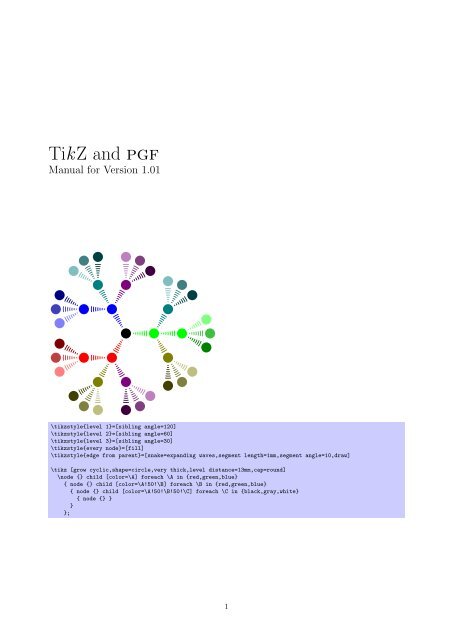
<strong>TikZ</strong> <strong>and</strong> <strong>pgf</strong><br />
Manual for Version 1.01<br />
\tikzstyle{level 1}=[sibling angle=120]<br />
\tikzstyle{level 2}=[sibling angle=60]<br />
\tikzstyle{level 3}=[sibling angle=30]<br />
\tikzstyle{every node}=[fill]<br />
\tikzstyle{edge from parent}=[snake=exp<strong>and</strong>ing waves,segment length=1mm,segment angle=10,draw]<br />
\tikz [grow cyclic,shape=circle,very thick,level distance=13mm,cap=round]<br />
\node {} child [color=\A] foreach \A in {red,green,blue}<br />
{ node {} child [color=\A!50!\B] foreach \B in {red,green,blue}<br />
{ node {} child [color=\A!50!\B!50!\C] foreach \C in {black,gray,white}<br />
{ node {} }<br />
}<br />
};<br />
1
Für meinen Vater, damit er noch viele schöne TEX-Graphiken erschaffen kann.<br />
2
The <strong>TikZ</strong> <strong>and</strong> <strong>pgf</strong> Packages<br />
Manual for Version 1.01<br />
http://sourceforge.net/projects/<strong>pgf</strong><br />
Till Tantau<br />
tantau@users.sourceforge.net<br />
November 16, 2005<br />
Contents<br />
I Getting Started 10<br />
1 Introduction 11<br />
1.1 Structure of the System . . . . . . . . . . . . . . . . . . . . . . . . . . . . . . . . . . . . . . . 11<br />
1.2 Comparison with Other Graphics Packages . . . . . . . . . . . . . . . . . . . . . . . . . . . . 12<br />
1.3 Utilities: Page Management . . . . . . . . . . . . . . . . . . . . . . . . . . . . . . . . . . . . 12<br />
1.4 How to Read This Manual . . . . . . . . . . . . . . . . . . . . . . . . . . . . . . . . . . . . . 12<br />
1.5 Getting Help . . . . . . . . . . . . . . . . . . . . . . . . . . . . . . . . . . . . . . . . . . . . . 13<br />
2 Installation 14<br />
2.1 Package <strong>and</strong> Driver Versions . . . . . . . . . . . . . . . . . . . . . . . . . . . . . . . . . . . . 14<br />
2.2 Installing Prebundled Packages . . . . . . . . . . . . . . . . . . . . . . . . . . . . . . . . . . 14<br />
2.2.1 Debian . . . . . . . . . . . . . . . . . . . . . . . . . . . . . . . . . . . . . . . . . . . . 14<br />
2.2.2 MiKTeX . . . . . . . . . . . . . . . . . . . . . . . . . . . . . . . . . . . . . . . . . . . 14<br />
2.3 Installation in a texmf Tree . . . . . . . . . . . . . . . . . . . . . . . . . . . . . . . . . . . . 15<br />
2.3.1 Installation that Keeps Everything Together . . . . . . . . . . . . . . . . . . . . . . . 15<br />
2.3.2 Installation that is TDS-Compliant . . . . . . . . . . . . . . . . . . . . . . . . . . . . 15<br />
2.4 Updating the Installation . . . . . . . . . . . . . . . . . . . . . . . . . . . . . . . . . . . . . . 15<br />
2.5 License: The GNU Public License, Version 2 . . . . . . . . . . . . . . . . . . . . . . . . . . . 15<br />
2.5.1 Preamble . . . . . . . . . . . . . . . . . . . . . . . . . . . . . . . . . . . . . . . . . . . 16<br />
2.5.2 Terms <strong>and</strong> Conditions For Copying, Distribution <strong>and</strong> Modification . . . . . . . . . . 16<br />
2.5.3 No Warranty . . . . . . . . . . . . . . . . . . . . . . . . . . . . . . . . . . . . . . . . 18<br />
3 Tutorial: A Picture for Karl’s Students 20<br />
3.1 Problem Statement . . . . . . . . . . . . . . . . . . . . . . . . . . . . . . . . . . . . . . . . . 20<br />
3.2 Setting up the Environment . . . . . . . . . . . . . . . . . . . . . . . . . . . . . . . . . . . . 20<br />
3.2.1 Setting up the Environment in L A TEX . . . . . . . . . . . . . . . . . . . . . . . . . . . 20<br />
3.2.2 Setting up the Environment in Plain TEX . . . . . . . . . . . . . . . . . . . . . . . . 21<br />
3.3 Straight Path Construction . . . . . . . . . . . . . . . . . . . . . . . . . . . . . . . . . . . . . 21<br />
3.4 Curved Path Construction . . . . . . . . . . . . . . . . . . . . . . . . . . . . . . . . . . . . . 22<br />
3.5 Circle Path Construction . . . . . . . . . . . . . . . . . . . . . . . . . . . . . . . . . . . . . . 22<br />
3.6 Rectangle Path Construction . . . . . . . . . . . . . . . . . . . . . . . . . . . . . . . . . . . . 23<br />
3.7 Grid Path Construction . . . . . . . . . . . . . . . . . . . . . . . . . . . . . . . . . . . . . . . 23<br />
3.8 Adding a Touch of Style . . . . . . . . . . . . . . . . . . . . . . . . . . . . . . . . . . . . . . 24<br />
3.9 Drawing Options . . . . . . . . . . . . . . . . . . . . . . . . . . . . . . . . . . . . . . . . . . 24<br />
3.10 Arc Path Construction . . . . . . . . . . . . . . . . . . . . . . . . . . . . . . . . . . . . . . . 25<br />
3.11 Clipping a Path . . . . . . . . . . . . . . . . . . . . . . . . . . . . . . . . . . . . . . . . . . . 26<br />
3.12 Parabola <strong>and</strong> Sine Path Construction . . . . . . . . . . . . . . . . . . . . . . . . . . . . . . . 27<br />
3.13 Filling <strong>and</strong> Drawing . . . . . . . . . . . . . . . . . . . . . . . . . . . . . . . . . . . . . . . . . 27<br />
3.14 Shading . . . . . . . . . . . . . . . . . . . . . . . . . . . . . . . . . . . . . . . . . . . . . . . 28<br />
3
3.15 Specifying Coordinates . . . . . . . . . . . . . . . . . . . . . . . . . . . . . . . . . . . . . . . 28<br />
3.16 Adding Arrow Tips . . . . . . . . . . . . . . . . . . . . . . . . . . . . . . . . . . . . . . . . . 30<br />
3.17 Scoping . . . . . . . . . . . . . . . . . . . . . . . . . . . . . . . . . . . . . . . . . . . . . . . . 31<br />
3.18 Transformations . . . . . . . . . . . . . . . . . . . . . . . . . . . . . . . . . . . . . . . . . . . 31<br />
3.19 Repeating Things: For-Loops . . . . . . . . . . . . . . . . . . . . . . . . . . . . . . . . . . . 32<br />
3.20 Adding Text . . . . . . . . . . . . . . . . . . . . . . . . . . . . . . . . . . . . . . . . . . . . . 33<br />
3.21 Nodes . . . . . . . . . . . . . . . . . . . . . . . . . . . . . . . . . . . . . . . . . . . . . . . . . 36<br />
4 Guidelines on Graphics 38<br />
4.1 Should You Follow Guidelines? . . . . . . . . . . . . . . . . . . . . . . . . . . . . . . . . . . . 38<br />
4.2 Planning the Time Needed for the Creation of Graphics . . . . . . . . . . . . . . . . . . . . 38<br />
4.3 Workflow for Creating a Graphic . . . . . . . . . . . . . . . . . . . . . . . . . . . . . . . . . 39<br />
4.4 Linking Graphics With the Main Text . . . . . . . . . . . . . . . . . . . . . . . . . . . . . . 39<br />
4.5 Consistency Between Graphics <strong>and</strong> Text . . . . . . . . . . . . . . . . . . . . . . . . . . . . . 40<br />
4.6 Labels in Graphics . . . . . . . . . . . . . . . . . . . . . . . . . . . . . . . . . . . . . . . . . 40<br />
4.7 Plots <strong>and</strong> Charts . . . . . . . . . . . . . . . . . . . . . . . . . . . . . . . . . . . . . . . . . . 41<br />
4.8 Attention <strong>and</strong> Distraction . . . . . . . . . . . . . . . . . . . . . . . . . . . . . . . . . . . . . 44<br />
5 Input <strong>and</strong> Output Formats 45<br />
5.1 Supported Input Formats . . . . . . . . . . . . . . . . . . . . . . . . . . . . . . . . . . . . . . 45<br />
5.1.1 Using the L A TEX Format . . . . . . . . . . . . . . . . . . . . . . . . . . . . . . . . . . 45<br />
5.1.2 Using the Plain TEX Format . . . . . . . . . . . . . . . . . . . . . . . . . . . . . . . . 45<br />
5.1.3 Using the ConTEXt Format . . . . . . . . . . . . . . . . . . . . . . . . . . . . . . . . 45<br />
5.2 Supported Output Formats . . . . . . . . . . . . . . . . . . . . . . . . . . . . . . . . . . . . . 45<br />
5.2.1 Selecting the Backend Driver . . . . . . . . . . . . . . . . . . . . . . . . . . . . . . . 46<br />
5.2.2 Producing PDF Output . . . . . . . . . . . . . . . . . . . . . . . . . . . . . . . . . . 46<br />
5.2.3 Producing PostScript Output . . . . . . . . . . . . . . . . . . . . . . . . . . . . . . . 47<br />
5.2.4 Producing HTML / SVG Output . . . . . . . . . . . . . . . . . . . . . . . . . . . . . 47<br />
II <strong>TikZ</strong> ist kein Zeichenprogramm 48<br />
6 Design Principles 49<br />
6.1 Special Syntax For Specifying Points . . . . . . . . . . . . . . . . . . . . . . . . . . . . . . . 49<br />
6.2 Special Syntax For Path Specifications . . . . . . . . . . . . . . . . . . . . . . . . . . . . . . 49<br />
6.3 Actions on Paths . . . . . . . . . . . . . . . . . . . . . . . . . . . . . . . . . . . . . . . . . . 49<br />
6.4 Key-Value Syntax for Graphic Parameters . . . . . . . . . . . . . . . . . . . . . . . . . . . . 50<br />
6.5 Special Syntax for Specifying Nodes . . . . . . . . . . . . . . . . . . . . . . . . . . . . . . . . 50<br />
6.6 Special Syntax for Specifying Trees . . . . . . . . . . . . . . . . . . . . . . . . . . . . . . . . 50<br />
6.7 Grouping of Graphic Parameters . . . . . . . . . . . . . . . . . . . . . . . . . . . . . . . . . 51<br />
6.8 Coordinate Transformation System . . . . . . . . . . . . . . . . . . . . . . . . . . . . . . . . 51<br />
7 Hierarchical Structures: Package, Environments, Scopes, <strong>and</strong> Styles 52<br />
7.1 Loading the Package . . . . . . . . . . . . . . . . . . . . . . . . . . . . . . . . . . . . . . . . 52<br />
7.2 Creating a Picture . . . . . . . . . . . . . . . . . . . . . . . . . . . . . . . . . . . . . . . . . . 52<br />
7.2.1 Creating a Picture Using an Environment . . . . . . . . . . . . . . . . . . . . . . . . 52<br />
7.2.2 Creating a Picture Using a Comm<strong>and</strong> . . . . . . . . . . . . . . . . . . . . . . . . . . . 53<br />
7.2.3 Adding a Background . . . . . . . . . . . . . . . . . . . . . . . . . . . . . . . . . . . . 54<br />
7.3 Using Scopes to Structure a Picture . . . . . . . . . . . . . . . . . . . . . . . . . . . . . . . . 54<br />
7.4 Using Scopes Inside Paths . . . . . . . . . . . . . . . . . . . . . . . . . . . . . . . . . . . . . 54<br />
7.5 Using Styles to Manage How Pictures Look . . . . . . . . . . . . . . . . . . . . . . . . . . . 55<br />
8 Specifying Coordinates 56<br />
8.1 Coordinates <strong>and</strong> Coordinate Options . . . . . . . . . . . . . . . . . . . . . . . . . . . . . . . 56<br />
8.2 Simple Coordinates . . . . . . . . . . . . . . . . . . . . . . . . . . . . . . . . . . . . . . . . . 56<br />
8.3 Polar Coordinates . . . . . . . . . . . . . . . . . . . . . . . . . . . . . . . . . . . . . . . . . . 56<br />
8.4 Xy- <strong>and</strong> Xyz-Coordinates . . . . . . . . . . . . . . . . . . . . . . . . . . . . . . . . . . . . . . 56<br />
8.5 Node Coordinates . . . . . . . . . . . . . . . . . . . . . . . . . . . . . . . . . . . . . . . . . . 56<br />
8.5.1 Named Anchor Coordinates . . . . . . . . . . . . . . . . . . . . . . . . . . . . . . . . 57<br />
4
8.5.2 Angle Anchor Coordinates . . . . . . . . . . . . . . . . . . . . . . . . . . . . . . . . . 57<br />
8.5.3 Anchor-Free Node Coordinates . . . . . . . . . . . . . . . . . . . . . . . . . . . . . . 57<br />
8.6 Intersection Coordinates . . . . . . . . . . . . . . . . . . . . . . . . . . . . . . . . . . . . . . 58<br />
8.6.1 Intersection of Two Lines . . . . . . . . . . . . . . . . . . . . . . . . . . . . . . . . . . 58<br />
8.6.2 Intersection of Horizontal <strong>and</strong> Vertical Lines . . . . . . . . . . . . . . . . . . . . . . . 58<br />
8.7 Relative <strong>and</strong> Incremental Coordinates . . . . . . . . . . . . . . . . . . . . . . . . . . . . . . . 59<br />
9 Syntax for Path Specifications 60<br />
9.1 The Move-To Operation . . . . . . . . . . . . . . . . . . . . . . . . . . . . . . . . . . . . . . 61<br />
9.2 The Line-To Operation . . . . . . . . . . . . . . . . . . . . . . . . . . . . . . . . . . . . . . . 61<br />
9.2.1 Straight Lines . . . . . . . . . . . . . . . . . . . . . . . . . . . . . . . . . . . . . . . . 61<br />
9.2.2 Horizontal <strong>and</strong> Vertical Lines . . . . . . . . . . . . . . . . . . . . . . . . . . . . . . . 61<br />
9.2.3 Snaked Lines . . . . . . . . . . . . . . . . . . . . . . . . . . . . . . . . . . . . . . . . 62<br />
9.3 The Curve-To Operation . . . . . . . . . . . . . . . . . . . . . . . . . . . . . . . . . . . . . . 65<br />
9.4 The Cycle Operation . . . . . . . . . . . . . . . . . . . . . . . . . . . . . . . . . . . . . . . . 66<br />
9.5 The Rectangle Operation . . . . . . . . . . . . . . . . . . . . . . . . . . . . . . . . . . . . . . 66<br />
9.6 Rounding Corners . . . . . . . . . . . . . . . . . . . . . . . . . . . . . . . . . . . . . . . . . . 66<br />
9.7 The Circle <strong>and</strong> Ellipse Operations . . . . . . . . . . . . . . . . . . . . . . . . . . . . . . . . . 67<br />
9.8 The Arc Operation . . . . . . . . . . . . . . . . . . . . . . . . . . . . . . . . . . . . . . . . . 67<br />
9.9 The Grid Operation . . . . . . . . . . . . . . . . . . . . . . . . . . . . . . . . . . . . . . . . . 68<br />
9.10 The Parabola Operation . . . . . . . . . . . . . . . . . . . . . . . . . . . . . . . . . . . . . . 69<br />
9.11 The Sine <strong>and</strong> Cosine Operation . . . . . . . . . . . . . . . . . . . . . . . . . . . . . . . . . . 70<br />
9.12 The Plot Operation . . . . . . . . . . . . . . . . . . . . . . . . . . . . . . . . . . . . . . . . . 70<br />
9.12.1 Plotting Points Given Inline . . . . . . . . . . . . . . . . . . . . . . . . . . . . . . . . 71<br />
9.12.2 Plotting Points Read From an External File . . . . . . . . . . . . . . . . . . . . . . . 71<br />
9.12.3 Plotting a Function . . . . . . . . . . . . . . . . . . . . . . . . . . . . . . . . . . . . . 71<br />
9.12.4 Placing Marks on the Plot . . . . . . . . . . . . . . . . . . . . . . . . . . . . . . . . . 74<br />
9.12.5 Smooth Plots, Sharp Plots, <strong>and</strong> Comb Plots . . . . . . . . . . . . . . . . . . . . . . . 74<br />
9.13 The Scoping Operation . . . . . . . . . . . . . . . . . . . . . . . . . . . . . . . . . . . . . . . 76<br />
9.14 The Node Operation . . . . . . . . . . . . . . . . . . . . . . . . . . . . . . . . . . . . . . . . 76<br />
10 Actions on Paths 77<br />
10.1 Specifying a Color . . . . . . . . . . . . . . . . . . . . . . . . . . . . . . . . . . . . . . . . . . 78<br />
10.2 Drawing a Path . . . . . . . . . . . . . . . . . . . . . . . . . . . . . . . . . . . . . . . . . . . 78<br />
10.2.1 Graphic Parameters: Line Width, Line Cap, <strong>and</strong> Line Join . . . . . . . . . . . . . . . 79<br />
10.2.2 Graphic Parameters: Dash Pattern . . . . . . . . . . . . . . . . . . . . . . . . . . . . 80<br />
10.2.3 Graphic Parameters: Draw Opacity . . . . . . . . . . . . . . . . . . . . . . . . . . . . 81<br />
10.2.4 Graphic Parameters: Arrow Tips . . . . . . . . . . . . . . . . . . . . . . . . . . . . . 82<br />
10.2.5 Graphic Parameters: Double Lines <strong>and</strong> Bordered Lines . . . . . . . . . . . . . . . . . 83<br />
10.3 Filling a Path . . . . . . . . . . . . . . . . . . . . . . . . . . . . . . . . . . . . . . . . . . . . 83<br />
10.3.1 Graphic Parameters: Interior Rules . . . . . . . . . . . . . . . . . . . . . . . . . . . . 84<br />
10.3.2 Graphic Parameters: Fill Opacity . . . . . . . . . . . . . . . . . . . . . . . . . . . . . 85<br />
10.4 Shading a Path . . . . . . . . . . . . . . . . . . . . . . . . . . . . . . . . . . . . . . . . . . . 86<br />
10.4.1 Choosing a Shading Type . . . . . . . . . . . . . . . . . . . . . . . . . . . . . . . . . 86<br />
10.4.2 Choosing a Shading Color . . . . . . . . . . . . . . . . . . . . . . . . . . . . . . . . . 87<br />
10.5 Establishing a Bounding Box . . . . . . . . . . . . . . . . . . . . . . . . . . . . . . . . . . . . 88<br />
10.6 Using a Path For Clipping . . . . . . . . . . . . . . . . . . . . . . . . . . . . . . . . . . . . . 89<br />
11 Nodes 91<br />
11.1 Nodes <strong>and</strong> Their Shapes . . . . . . . . . . . . . . . . . . . . . . . . . . . . . . . . . . . . . . 91<br />
11.2 Multi-Part Nodes . . . . . . . . . . . . . . . . . . . . . . . . . . . . . . . . . . . . . . . . . . 92<br />
11.3 Options for the Text in Nodes . . . . . . . . . . . . . . . . . . . . . . . . . . . . . . . . . . . 93<br />
11.4 Placing Nodes Using Anchors . . . . . . . . . . . . . . . . . . . . . . . . . . . . . . . . . . . 95<br />
11.5 Transformations . . . . . . . . . . . . . . . . . . . . . . . . . . . . . . . . . . . . . . . . . . . 97<br />
11.6 Placing Nodes on a Line or Curve . . . . . . . . . . . . . . . . . . . . . . . . . . . . . . . . . 97<br />
11.6.1 Explicit Use of the Position Option . . . . . . . . . . . . . . . . . . . . . . . . . . . . 97<br />
11.6.2 Implicit Use of the Position Option . . . . . . . . . . . . . . . . . . . . . . . . . . . . 99<br />
11.7 Connecting Nodes . . . . . . . . . . . . . . . . . . . . . . . . . . . . . . . . . . . . . . . . . . 99<br />
11.8 Predefined Shapes . . . . . . . . . . . . . . . . . . . . . . . . . . . . . . . . . . . . . . . . . . 100<br />
5
12 Making Trees Grow 103<br />
12.1 Introduction to the Child Operation . . . . . . . . . . . . . . . . . . . . . . . . . . . . . . . . 103<br />
12.2 Child Paths <strong>and</strong> the Child Nodes . . . . . . . . . . . . . . . . . . . . . . . . . . . . . . . . . 104<br />
12.3 Naming Child Nodes . . . . . . . . . . . . . . . . . . . . . . . . . . . . . . . . . . . . . . . . 104<br />
12.4 Specifying Options for Trees <strong>and</strong> Children . . . . . . . . . . . . . . . . . . . . . . . . . . . . 105<br />
12.5 Placing Child Nodes . . . . . . . . . . . . . . . . . . . . . . . . . . . . . . . . . . . . . . . . 106<br />
12.6 Edges From the Parent Node . . . . . . . . . . . . . . . . . . . . . . . . . . . . . . . . . . . . 109<br />
13 Transformations 112<br />
13.1 The Different Coordinate Systems . . . . . . . . . . . . . . . . . . . . . . . . . . . . . . . . . 112<br />
13.2 The Xy- <strong>and</strong> Xyz-Coordinate Systems . . . . . . . . . . . . . . . . . . . . . . . . . . . . . . 112<br />
13.3 Coordinate Transformations . . . . . . . . . . . . . . . . . . . . . . . . . . . . . . . . . . . . 113<br />
III Libraries <strong>and</strong> Utilities 116<br />
14 Libraries 117<br />
14.1 Arrow Tip Library . . . . . . . . . . . . . . . . . . . . . . . . . . . . . . . . . . . . . . . . . 117<br />
14.1.1 Triangular Arrow Tips . . . . . . . . . . . . . . . . . . . . . . . . . . . . . . . . . . . 117<br />
14.1.2 Barbed Arrow Tips . . . . . . . . . . . . . . . . . . . . . . . . . . . . . . . . . . . . . 117<br />
14.1.3 Bracket-Like Arrow Tips . . . . . . . . . . . . . . . . . . . . . . . . . . . . . . . . . . 117<br />
14.1.4 Circle <strong>and</strong> Diamond Arrow Tips . . . . . . . . . . . . . . . . . . . . . . . . . . . . . . 117<br />
14.1.5 Partial Arrow Tips . . . . . . . . . . . . . . . . . . . . . . . . . . . . . . . . . . . . . 118<br />
14.1.6 Line Caps . . . . . . . . . . . . . . . . . . . . . . . . . . . . . . . . . . . . . . . . . . 118<br />
14.2 Snake Library . . . . . . . . . . . . . . . . . . . . . . . . . . . . . . . . . . . . . . . . . . . . 118<br />
14.3 Plot H<strong>and</strong>ler Library . . . . . . . . . . . . . . . . . . . . . . . . . . . . . . . . . . . . . . . . 120<br />
14.3.1 Curve Plot H<strong>and</strong>lers . . . . . . . . . . . . . . . . . . . . . . . . . . . . . . . . . . . . 121<br />
14.3.2 Comb Plot H<strong>and</strong>lers . . . . . . . . . . . . . . . . . . . . . . . . . . . . . . . . . . . . 121<br />
14.3.3 Mark Plot H<strong>and</strong>ler . . . . . . . . . . . . . . . . . . . . . . . . . . . . . . . . . . . . . 122<br />
14.4 Plot Mark Library . . . . . . . . . . . . . . . . . . . . . . . . . . . . . . . . . . . . . . . . . . 123<br />
14.5 Shape Library . . . . . . . . . . . . . . . . . . . . . . . . . . . . . . . . . . . . . . . . . . . . 124<br />
14.6 Tree Library . . . . . . . . . . . . . . . . . . . . . . . . . . . . . . . . . . . . . . . . . . . . . 126<br />
14.6.1 Growth Functions . . . . . . . . . . . . . . . . . . . . . . . . . . . . . . . . . . . . . . 126<br />
14.6.2 Edges From Parent . . . . . . . . . . . . . . . . . . . . . . . . . . . . . . . . . . . . . 128<br />
14.7 Background Library . . . . . . . . . . . . . . . . . . . . . . . . . . . . . . . . . . . . . . . . . 129<br />
14.8 Automata Drawing Library . . . . . . . . . . . . . . . . . . . . . . . . . . . . . . . . . . . . 131<br />
15 Repeating Things: The Foreach Statement 133<br />
16 Page Management 137<br />
16.1 Basic Usage . . . . . . . . . . . . . . . . . . . . . . . . . . . . . . . . . . . . . . . . . . . . . 137<br />
16.2 The Predefined Layouts . . . . . . . . . . . . . . . . . . . . . . . . . . . . . . . . . . . . . . . 138<br />
16.3 Defining a Layout . . . . . . . . . . . . . . . . . . . . . . . . . . . . . . . . . . . . . . . . . . 140<br />
16.4 Creating Logical Pages . . . . . . . . . . . . . . . . . . . . . . . . . . . . . . . . . . . . . . . 143<br />
17 Extended Color Support 144<br />
IV The Basic Layer 145<br />
18 Design Principles 146<br />
18.1 Core <strong>and</strong> Optional Packages . . . . . . . . . . . . . . . . . . . . . . . . . . . . . . . . . . . . 146<br />
18.2 Communicating with the Basic Layer via Macros . . . . . . . . . . . . . . . . . . . . . . . . 146<br />
18.3 Path-Centered Approach . . . . . . . . . . . . . . . . . . . . . . . . . . . . . . . . . . . . . . 147<br />
18.4 Coordinate Versus Canvas Transformations . . . . . . . . . . . . . . . . . . . . . . . . . . . . 147<br />
6
19 Hierarchical Structures: Package, Environments, Scopes, <strong>and</strong> Text 148<br />
19.1 Overview . . . . . . . . . . . . . . . . . . . . . . . . . . . . . . . . . . . . . . . . . . . . . . . 148<br />
19.1.1 The Hierarchical Structure of the Package . . . . . . . . . . . . . . . . . . . . . . . . 148<br />
19.1.2 The Hierarchical Structure of Graphics . . . . . . . . . . . . . . . . . . . . . . . . . . 148<br />
19.2 The Hierarchical Structure of the Package . . . . . . . . . . . . . . . . . . . . . . . . . . . . 149<br />
19.2.1 The Main Package . . . . . . . . . . . . . . . . . . . . . . . . . . . . . . . . . . . . . 149<br />
19.2.2 The Core Package . . . . . . . . . . . . . . . . . . . . . . . . . . . . . . . . . . . . . . 150<br />
19.2.3 The Optional Basic Layer Packages . . . . . . . . . . . . . . . . . . . . . . . . . . . . 150<br />
19.3 The Hierarchical Structure of the Graphics . . . . . . . . . . . . . . . . . . . . . . . . . . . . 150<br />
19.3.1 The Main Environment . . . . . . . . . . . . . . . . . . . . . . . . . . . . . . . . . . . 150<br />
19.3.2 Graphic Scope Environments . . . . . . . . . . . . . . . . . . . . . . . . . . . . . . . 151<br />
19.3.3 Inserting Text <strong>and</strong> Images . . . . . . . . . . . . . . . . . . . . . . . . . . . . . . . . . 153<br />
20 Specifying Coordinates 155<br />
20.1 Overview . . . . . . . . . . . . . . . . . . . . . . . . . . . . . . . . . . . . . . . . . . . . . . . 155<br />
20.2 Basic Coordinate Comm<strong>and</strong>s . . . . . . . . . . . . . . . . . . . . . . . . . . . . . . . . . . . . 155<br />
20.3 Coordinates in the Xy- <strong>and</strong> Xyz-Coordinate Systems . . . . . . . . . . . . . . . . . . . . . . 155<br />
20.4 Building Coordinates From Other Coordinates . . . . . . . . . . . . . . . . . . . . . . . . . . 156<br />
20.4.1 Basic Manipulations of Coordinates . . . . . . . . . . . . . . . . . . . . . . . . . . . . 156<br />
20.4.2 Points Traveling along Lines <strong>and</strong> Curves . . . . . . . . . . . . . . . . . . . . . . . . . 157<br />
20.4.3 Points on Borders of Objects . . . . . . . . . . . . . . . . . . . . . . . . . . . . . . . . 158<br />
20.4.4 Points on the Intersection of Lines . . . . . . . . . . . . . . . . . . . . . . . . . . . . 159<br />
20.5 Extracting Coordinates . . . . . . . . . . . . . . . . . . . . . . . . . . . . . . . . . . . . . . . 159<br />
20.6 Internals of How Point Comm<strong>and</strong>s Work . . . . . . . . . . . . . . . . . . . . . . . . . . . . . 159<br />
21 Constructing Paths 161<br />
21.1 Overview . . . . . . . . . . . . . . . . . . . . . . . . . . . . . . . . . . . . . . . . . . . . . . . 161<br />
21.2 The Move-To Path Operation . . . . . . . . . . . . . . . . . . . . . . . . . . . . . . . . . . . 161<br />
21.3 The Line-To Path Operation . . . . . . . . . . . . . . . . . . . . . . . . . . . . . . . . . . . . 162<br />
21.4 The Curve-To Path Operation . . . . . . . . . . . . . . . . . . . . . . . . . . . . . . . . . . . 162<br />
21.5 The Close Path Operation . . . . . . . . . . . . . . . . . . . . . . . . . . . . . . . . . . . . . 163<br />
21.6 Arc, Ellipse <strong>and</strong> Circle Path Operations . . . . . . . . . . . . . . . . . . . . . . . . . . . . . 163<br />
21.7 Rectangle Path Operations . . . . . . . . . . . . . . . . . . . . . . . . . . . . . . . . . . . . . 164<br />
21.8 The Grid Path Operation . . . . . . . . . . . . . . . . . . . . . . . . . . . . . . . . . . . . . . 165<br />
21.9 The Parabola Path Operation . . . . . . . . . . . . . . . . . . . . . . . . . . . . . . . . . . . 165<br />
21.10 Sine <strong>and</strong> Cosine Path Operations . . . . . . . . . . . . . . . . . . . . . . . . . . . . . . . . . 166<br />
21.11 Plot Path Operations . . . . . . . . . . . . . . . . . . . . . . . . . . . . . . . . . . . . . . . . 166<br />
21.12 Rounded Corners . . . . . . . . . . . . . . . . . . . . . . . . . . . . . . . . . . . . . . . . . . 167<br />
21.13 Internal Tracking of Bounding Boxes for Paths <strong>and</strong> Pictures . . . . . . . . . . . . . . . . . . 167<br />
22 Snakes 169<br />
22.1 Overview . . . . . . . . . . . . . . . . . . . . . . . . . . . . . . . . . . . . . . . . . . . . . . . 169<br />
22.2 Declaring a Snake . . . . . . . . . . . . . . . . . . . . . . . . . . . . . . . . . . . . . . . . . . 169<br />
22.2.1 Segments . . . . . . . . . . . . . . . . . . . . . . . . . . . . . . . . . . . . . . . . . . . 169<br />
22.2.2 Snake Automata . . . . . . . . . . . . . . . . . . . . . . . . . . . . . . . . . . . . . . 169<br />
22.2.3 The Snake Declaration Comm<strong>and</strong> . . . . . . . . . . . . . . . . . . . . . . . . . . . . . 170<br />
22.2.4 Predefined Snakes . . . . . . . . . . . . . . . . . . . . . . . . . . . . . . . . . . . . . . 171<br />
22.3 Using Snakes . . . . . . . . . . . . . . . . . . . . . . . . . . . . . . . . . . . . . . . . . . . . . 172<br />
23 Using Paths 174<br />
23.1 Overview . . . . . . . . . . . . . . . . . . . . . . . . . . . . . . . . . . . . . . . . . . . . . . . 174<br />
23.2 Stroking a Path . . . . . . . . . . . . . . . . . . . . . . . . . . . . . . . . . . . . . . . . . . . 175<br />
23.2.1 Graphic Parameter: Line Width . . . . . . . . . . . . . . . . . . . . . . . . . . . . . . 175<br />
23.2.2 Graphic Parameter: Caps <strong>and</strong> Joins . . . . . . . . . . . . . . . . . . . . . . . . . . . . 175<br />
23.2.3 Graphic Parameter: Dashing . . . . . . . . . . . . . . . . . . . . . . . . . . . . . . . . 175<br />
23.2.4 Graphic Parameter: Stroke Color . . . . . . . . . . . . . . . . . . . . . . . . . . . . . 176<br />
23.2.5 Graphic Parameter: Stroke Opacity . . . . . . . . . . . . . . . . . . . . . . . . . . . . 176<br />
23.2.6 Graphic Parameter: Arrows . . . . . . . . . . . . . . . . . . . . . . . . . . . . . . . . 177<br />
23.3 Filling a Path . . . . . . . . . . . . . . . . . . . . . . . . . . . . . . . . . . . . . . . . . . . . 178<br />
7
23.3.1 Graphic Parameter: Interior Rule . . . . . . . . . . . . . . . . . . . . . . . . . . . . . 178<br />
23.3.2 Graphic Parameter: Filling Color . . . . . . . . . . . . . . . . . . . . . . . . . . . . . 178<br />
23.3.3 Graphic Parameter: Fill Opacity . . . . . . . . . . . . . . . . . . . . . . . . . . . . . 178<br />
23.4 Clipping a Path . . . . . . . . . . . . . . . . . . . . . . . . . . . . . . . . . . . . . . . . . . . 178<br />
23.5 Using a Path as a Bounding Box . . . . . . . . . . . . . . . . . . . . . . . . . . . . . . . . . 179<br />
24 Arrow Tips 180<br />
24.1 Overview . . . . . . . . . . . . . . . . . . . . . . . . . . . . . . . . . . . . . . . . . . . . . . . 180<br />
24.1.1 When Does PGF Draw Arrow Tips? . . . . . . . . . . . . . . . . . . . . . . . . . . . 180<br />
24.1.2 Meta-Arrow Tips . . . . . . . . . . . . . . . . . . . . . . . . . . . . . . . . . . . . . . 180<br />
24.2 Declaring an Arrow Tip Kind . . . . . . . . . . . . . . . . . . . . . . . . . . . . . . . . . . . 181<br />
24.3 Declaring a Derived Arrow Tip Kind . . . . . . . . . . . . . . . . . . . . . . . . . . . . . . . 183<br />
24.4 Using an Arrow Tip Kind . . . . . . . . . . . . . . . . . . . . . . . . . . . . . . . . . . . . . 185<br />
24.5 Predefined Arrow Tip Kinds . . . . . . . . . . . . . . . . . . . . . . . . . . . . . . . . . . . . 186<br />
25 Nodes <strong>and</strong> Shapes 187<br />
25.1 Overview . . . . . . . . . . . . . . . . . . . . . . . . . . . . . . . . . . . . . . . . . . . . . . . 187<br />
25.1.1 Creating <strong>and</strong> Referencing Nodes . . . . . . . . . . . . . . . . . . . . . . . . . . . . . . 187<br />
25.1.2 Anchors . . . . . . . . . . . . . . . . . . . . . . . . . . . . . . . . . . . . . . . . . . . 187<br />
25.1.3 Layers of a Shape . . . . . . . . . . . . . . . . . . . . . . . . . . . . . . . . . . . . . . 187<br />
25.1.4 Node Parts . . . . . . . . . . . . . . . . . . . . . . . . . . . . . . . . . . . . . . . . . . 188<br />
25.2 Creating Nodes . . . . . . . . . . . . . . . . . . . . . . . . . . . . . . . . . . . . . . . . . . . 188<br />
25.3 Using Anchors . . . . . . . . . . . . . . . . . . . . . . . . . . . . . . . . . . . . . . . . . . . . 191<br />
25.4 Declaring New Shapes . . . . . . . . . . . . . . . . . . . . . . . . . . . . . . . . . . . . . . . 192<br />
25.4.1 What Must Be Defined For a Shape? . . . . . . . . . . . . . . . . . . . . . . . . . . . 192<br />
25.4.2 Normal Anchors Versus Saved Anchors . . . . . . . . . . . . . . . . . . . . . . . . . . 192<br />
25.4.3 Comm<strong>and</strong> for Declaring New Shapes . . . . . . . . . . . . . . . . . . . . . . . . . . . 192<br />
25.5 Predefined Shapes . . . . . . . . . . . . . . . . . . . . . . . . . . . . . . . . . . . . . . . . . . 197<br />
26 Coordinate <strong>and</strong> Canvas Transformations 200<br />
26.1 Overview . . . . . . . . . . . . . . . . . . . . . . . . . . . . . . . . . . . . . . . . . . . . . . . 200<br />
26.2 Coordinate Transformations . . . . . . . . . . . . . . . . . . . . . . . . . . . . . . . . . . . . 200<br />
26.2.1 How PGF Keeps Track of the Coordinate Transformation Matrix . . . . . . . . . . . 200<br />
26.2.2 Comm<strong>and</strong>s for Relative Coordinate Transformations . . . . . . . . . . . . . . . . . . 200<br />
26.2.3 Comm<strong>and</strong>s for Absolute Coordinate Transformations . . . . . . . . . . . . . . . . . . 203<br />
26.2.4 Saving <strong>and</strong> Restoring the Coordinate Transformation Matrix . . . . . . . . . . . . . . 204<br />
26.3 Canvas Transformations . . . . . . . . . . . . . . . . . . . . . . . . . . . . . . . . . . . . . . 204<br />
27 Declaring <strong>and</strong> Using Images 207<br />
27.1 Overview . . . . . . . . . . . . . . . . . . . . . . . . . . . . . . . . . . . . . . . . . . . . . . . 207<br />
27.2 Declaring an Image . . . . . . . . . . . . . . . . . . . . . . . . . . . . . . . . . . . . . . . . . 207<br />
27.3 Using an Image . . . . . . . . . . . . . . . . . . . . . . . . . . . . . . . . . . . . . . . . . . . 208<br />
27.4 Masking an Image . . . . . . . . . . . . . . . . . . . . . . . . . . . . . . . . . . . . . . . . . . 209<br />
28 Declaring <strong>and</strong> Using Shadings 211<br />
28.1 Overview . . . . . . . . . . . . . . . . . . . . . . . . . . . . . . . . . . . . . . . . . . . . . . . 211<br />
28.2 Declaring Shadings . . . . . . . . . . . . . . . . . . . . . . . . . . . . . . . . . . . . . . . . . 211<br />
28.3 Using Shadings . . . . . . . . . . . . . . . . . . . . . . . . . . . . . . . . . . . . . . . . . . . 212<br />
29 Creating Plots 216<br />
29.1 Overview . . . . . . . . . . . . . . . . . . . . . . . . . . . . . . . . . . . . . . . . . . . . . . . 216<br />
29.1.1 When Should One Use PGF for Generating Plots? . . . . . . . . . . . . . . . . . . . 216<br />
29.1.2 How PGF H<strong>and</strong>les Plots . . . . . . . . . . . . . . . . . . . . . . . . . . . . . . . . . . 216<br />
29.2 Generating Plot Streams . . . . . . . . . . . . . . . . . . . . . . . . . . . . . . . . . . . . . . 217<br />
29.2.1 Basic Building Blocks of Plot Streams . . . . . . . . . . . . . . . . . . . . . . . . . . 217<br />
29.2.2 Comm<strong>and</strong>s That Generate Plot Streams . . . . . . . . . . . . . . . . . . . . . . . . . 217<br />
29.3 Plot H<strong>and</strong>lers . . . . . . . . . . . . . . . . . . . . . . . . . . . . . . . . . . . . . . . . . . . . 219<br />
8
30 Layered Graphics 220<br />
30.1 Overview . . . . . . . . . . . . . . . . . . . . . . . . . . . . . . . . . . . . . . . . . . . . . . . 220<br />
30.2 Declaring Layers . . . . . . . . . . . . . . . . . . . . . . . . . . . . . . . . . . . . . . . . . . . 220<br />
30.3 Using Layers . . . . . . . . . . . . . . . . . . . . . . . . . . . . . . . . . . . . . . . . . . . . . 220<br />
31 Quick Comm<strong>and</strong>s 222<br />
31.1 Quick Path Construction Comm<strong>and</strong>s . . . . . . . . . . . . . . . . . . . . . . . . . . . . . . . 222<br />
31.2 Quick Path Usage Comm<strong>and</strong>s . . . . . . . . . . . . . . . . . . . . . . . . . . . . . . . . . . . 223<br />
31.3 Quick Text Box Comm<strong>and</strong>s . . . . . . . . . . . . . . . . . . . . . . . . . . . . . . . . . . . . 223<br />
V The System Layer 224<br />
32 Design of the System Layer 225<br />
32.1 Driver Files . . . . . . . . . . . . . . . . . . . . . . . . . . . . . . . . . . . . . . . . . . . . . 225<br />
32.2 Common Definition Files . . . . . . . . . . . . . . . . . . . . . . . . . . . . . . . . . . . . . . 225<br />
33 Comm<strong>and</strong>s of the System Layer 226<br />
33.1 Beginning <strong>and</strong> Ending a Stream of System Comm<strong>and</strong>s . . . . . . . . . . . . . . . . . . . . . 226<br />
33.2 Path Construction System Comm<strong>and</strong>s . . . . . . . . . . . . . . . . . . . . . . . . . . . . . . 227<br />
33.3 Canvas Transformation System Comm<strong>and</strong>s . . . . . . . . . . . . . . . . . . . . . . . . . . . . 228<br />
33.4 Stroking, Filling, <strong>and</strong> Clipping System Comm<strong>and</strong>s . . . . . . . . . . . . . . . . . . . . . . . . 228<br />
33.5 Graphic State Option System Comm<strong>and</strong>s . . . . . . . . . . . . . . . . . . . . . . . . . . . . . 229<br />
33.6 Color System Comm<strong>and</strong>s . . . . . . . . . . . . . . . . . . . . . . . . . . . . . . . . . . . . . . 230<br />
33.7 Scoping System Comm<strong>and</strong>s . . . . . . . . . . . . . . . . . . . . . . . . . . . . . . . . . . . . 232<br />
33.8 Image System Comm<strong>and</strong>s . . . . . . . . . . . . . . . . . . . . . . . . . . . . . . . . . . . . . 232<br />
33.9 Shading System Comm<strong>and</strong>s . . . . . . . . . . . . . . . . . . . . . . . . . . . . . . . . . . . . 233<br />
33.10 Reusable Objects System Comm<strong>and</strong>s . . . . . . . . . . . . . . . . . . . . . . . . . . . . . . . 234<br />
33.11 Invisibility System Comm<strong>and</strong>s . . . . . . . . . . . . . . . . . . . . . . . . . . . . . . . . . . . 234<br />
33.12 Internal Conversion Comm<strong>and</strong>s . . . . . . . . . . . . . . . . . . . . . . . . . . . . . . . . . . 234<br />
34 The Soft Path Subsystem 235<br />
34.1 Path Creation Process . . . . . . . . . . . . . . . . . . . . . . . . . . . . . . . . . . . . . . . 235<br />
34.2 Starting <strong>and</strong> Ending a Soft Path . . . . . . . . . . . . . . . . . . . . . . . . . . . . . . . . . . 235<br />
34.3 Soft Path Creation Comm<strong>and</strong>s . . . . . . . . . . . . . . . . . . . . . . . . . . . . . . . . . . . 236<br />
34.4 The Soft Path Data Structure . . . . . . . . . . . . . . . . . . . . . . . . . . . . . . . . . . . 236<br />
35 The Protocol Subsystem 238<br />
VI References <strong>and</strong> Index 239<br />
Index 240<br />
9
Part I<br />
Getting Started<br />
This part is intended to help you get started with the <strong>pgf</strong> package. First, the installation process is explained;<br />
however, the system will typically be already installed on your system, so this can often be skipped. Next,<br />
a short tutorial is given that explains the most often used comm<strong>and</strong>s <strong>and</strong> concepts of <strong>TikZ</strong>, without going<br />
into any of the glorious details. At the end of this section you will find some, hopefully useful, hints on how<br />
to create “good” graphics in general. The information in this section is not specific to <strong>pgf</strong>.<br />
\tikz \draw[thick,rounded corners=8pt]<br />
(0,0) -- (0,2) -- (1,3.25) -- (2,2) -- (2,0) -- (0,2) -- (2,2) -- (0,0) -- (2,0);<br />
10
1 Introduction<br />
The <strong>pgf</strong> package, where “<strong>pgf</strong>” is supposed to mean “portable graphics format” (or “pretty, good, functional”<br />
if you prefer. . . ), is a package for creating graphics in an “inline” manner. The package defines a number<br />
of TEX comm<strong>and</strong>s that draw graphics. For example, the code \tikz \draw (0pt,0pt) -- (20pt,6pt);<br />
yields the line <strong>and</strong> the code \tikz \fill[orange] (1ex,1ex) circle (1ex); yields .<br />
In a sense, when using <strong>pgf</strong> you “program” your graphics, just as you “program” your document when<br />
using TEX. This means that you get the advantages of the “TEX-approach to typesetting” also for your<br />
graphics: quick creation of simple graphics, precise positioning, the use of macros, often superior typography.<br />
You also inherit all the disadvantages: steep learning curve, no wysiwyg, small changes require a long<br />
recompilation time, <strong>and</strong> the code does not really “show” how things will look like.<br />
1.1 Structure of the System<br />
The <strong>pgf</strong> system consists of different layers:<br />
System layer: This layer provides a complete abstraction of what is going on “in the driver.” The driver<br />
is a program like dvips or dvipdfm that takes a .dvi file as input <strong>and</strong> generates a .ps or a .pdf file.<br />
(The pdftex program also counts as a driver, even though it does not take a .dvi file as input. Never<br />
mind.) Each driver has its own syntax for the generation of graphics, causing headaches to everyone<br />
who wants to create graphics in a portable way. <strong>pgf</strong>’s system layer “abstracts away” these differences.<br />
For example, the system comm<strong>and</strong> \<strong>pgf</strong>sys@lineto{10pt}{10pt} extends the current path to the<br />
coordinate (10pt, 10pt) of the current {<strong>pgf</strong>picture}. Depending on whether dvips, dvipdfm, or<br />
pdftex is used to process the document, the system comm<strong>and</strong> will be converted to different \special<br />
comm<strong>and</strong>s.<br />
The system layer is as “minimalistic” as possible since each additional comm<strong>and</strong> makes it more work to<br />
port <strong>pgf</strong> to a new driver. Currently, only drivers that produce PostScript or pdf output are supported<br />
<strong>and</strong> only few of these (hence the name portable graphics format is currently a bit boastful). However,<br />
in principle, the system layer could be ported to many different drivers quite easily. It should even be<br />
possible to produce, say, svg output in conjunction with tex4ht.<br />
As a user, you will not use the system layer directly.<br />
Basic layer: The basic layer provides a set of basic comm<strong>and</strong>s that allow you to produce complex graphics<br />
in a much easier way than by using the system layer directly. For example, the system layer provides<br />
no comm<strong>and</strong>s for creating circles since circles can be composed from the more basic Bézier curves (well,<br />
almost). However, as a user you will want to have a simple comm<strong>and</strong> to create circles (at least I do)<br />
instead of having to write down half a page of Bézier curve support coordinates. Thus, the basic layer<br />
provides a comm<strong>and</strong> \<strong>pgf</strong>pathcircle that generates the necessary curve coordinates for you.<br />
The basic layer is consists of a core, which consists of several interdependent packages that can only<br />
be loaded en bloc, <strong>and</strong> additional packages that extend the core by more special-purpose comm<strong>and</strong>s<br />
like node management or a plotting interface. For instance, the beamer package uses the core, but<br />
not all of the additional packages of the basic layer.<br />
Frontend layer: A frontend (of which there can be several) is a set of comm<strong>and</strong>s or a special syntax that<br />
makes using the basic layer easier. A problem with directly using the basic layer is that code written<br />
for this layer is often too “verbose.” For example, to draw a simple triangle, you may need as many as<br />
five comm<strong>and</strong>s when using the basic layer: One for beginning a path at the first corner of the triangle,<br />
one for extending the path to the second corner, one for going to the third, one for closing the path,<br />
<strong>and</strong> one for actually painting the triangle (as opposed to filling it). With the tikz frontend all this<br />
boils down to a single simple metafont-like comm<strong>and</strong>:<br />
\draw (0,0) -- (1,0) -- (1,1) -- cycle;<br />
There are different frontends:<br />
• The <strong>TikZ</strong> frontend is the “natural” frontend for <strong>pgf</strong>. It gives you access to all features of <strong>pgf</strong>,<br />
but it is intended to be easy to use. The syntax is a mixture of metafont <strong>and</strong> pstricks <strong>and</strong><br />
some ideas of myself. This frontend is neither a complete metafont compatibility layer nor a<br />
pstricks compatibility layer <strong>and</strong> it is not intended to become either.<br />
11
• The <strong>pgf</strong>pict2e frontend reimplements the st<strong>and</strong>ard L A TEX {picture} environment <strong>and</strong> comm<strong>and</strong>s<br />
like \line or \vector using the <strong>pgf</strong> basic layer. This layer is not really “necessary” since<br />
the pict2e.sty package does at least as good a job at reimplementing the {picture} environment.<br />
Rather, the idea behind this package is to have a simple demonstration of how a frontend<br />
can be implemented.<br />
It would be possible to implement a <strong>pgf</strong>tricks frontend that maps pstricks comm<strong>and</strong>s to <strong>pgf</strong><br />
comm<strong>and</strong>s. However, I have not done this <strong>and</strong> even if fully implemented, many things that work in<br />
pstricks will not work, namely whenever some pstricks comm<strong>and</strong> relies too heavily on PostScript<br />
trickery. Nevertheless, such a package might be useful in some situations.<br />
As a user of <strong>pgf</strong> you will use the comm<strong>and</strong>s of a frontend plus perhaps some comm<strong>and</strong>s of the basic<br />
layer. For this reason, this manual explains the frontends first, then the basic layer, <strong>and</strong> finally the system<br />
layer.<br />
1.2 Comparison with Other Graphics Packages<br />
There were two main motivations for creating <strong>pgf</strong>:<br />
1. The st<strong>and</strong>ard L A TEX {picture} environment is not powerful enough to create anything but really<br />
simple graphics. This is certainly not due to a lack of knowledge or imagination on the part of L A TEX’s<br />
designer(s). Rather, this is the price paid for the {picture} environment’s portability: It works<br />
together with all backend drivers.<br />
2. The {pstricks} package is certainly powerful enough to create any conceivable kind of graphic, but<br />
it is not portable at all. Most importantly, it does not work with pdftex nor with any other driver<br />
that produces anything but PostScript code.<br />
The <strong>pgf</strong> package is a trade-off between portability <strong>and</strong> expressive power. It is not as portable as<br />
{picture} <strong>and</strong> perhaps not quite as powerful as {pspicture}. However, it is more powerful than {picture}<br />
<strong>and</strong> more portable than {pspicture}.<br />
1.3 Utilities: Page Management<br />
The <strong>pgf</strong> package include a special subpackage called <strong>pgf</strong>pages, which is used to assemble several pages into<br />
a single page. This package is not really about creating graphics, but it is part of <strong>pgf</strong> nevertheless, mostly<br />
because its implementation uses <strong>pgf</strong> heavily.<br />
The subpackage <strong>pgf</strong>pages provides comm<strong>and</strong>s for assembling several “virtual pages” into a single “physical<br />
page.” The idea is that whenever TEX has a page ready for “shipout,” <strong>pgf</strong>pages interrupts this shipout<br />
<strong>and</strong> instead stores the page to be shipped out in a special box. When enough “virtual pages” have been<br />
accumulated in this way, they are scaled down <strong>and</strong> arranged on a “physical page,” which then really shipped<br />
out. This mechanism allows you to create “two page on one page” versions of a document directly inside<br />
L A TEX without the use of any external programs.<br />
However, <strong>pgf</strong>pages can do quite a lot more than that. You can use it to put logos <strong>and</strong> watermark on<br />
pages, print up to 16 pages on one page, add borders to pages, <strong>and</strong> more.<br />
1.4 How to Read This Manual<br />
This manual describes both the design of the <strong>pgf</strong> system <strong>and</strong> its usage. The organization is very roughly<br />
according to “user-friendliness.” The comm<strong>and</strong>s <strong>and</strong> subpackages that are easiest <strong>and</strong> most frequently used<br />
are described first, more low-level <strong>and</strong> esoteric features are discussed later.<br />
If you have not yet installed <strong>pgf</strong>, please read the installation first. Second, it might be a good idea to<br />
read the tutorial. Finally, you might wish to skim through the description of <strong>TikZ</strong>. Typically, you will not<br />
need to read the sections on the basic layer. You will only need to read the part on the system layer if you<br />
intend to write your own frontend or if you wish to port <strong>pgf</strong> to a new driver.<br />
The “public” comm<strong>and</strong>s <strong>and</strong> environments provided by the <strong>pgf</strong> package are described throughout the<br />
text. In each such description, the described comm<strong>and</strong>, environment or option is printed in red. Text shown<br />
in green is optional <strong>and</strong> can be left out.<br />
12
1.5 Getting Help<br />
When you need help with <strong>pgf</strong> <strong>and</strong> <strong>TikZ</strong>, please do the following:<br />
1. Read the manual, at least the part that has to do with your problem.<br />
2. If that does not solve the problem, try having a look at the sourceforge development page for <strong>pgf</strong> <strong>and</strong><br />
<strong>TikZ</strong> (see the title of this document). Perhaps someone has already reported a similar problem <strong>and</strong><br />
someone has found a solution.<br />
3. On the website you will find numerous forums for getting help. There, you can write to help forums,<br />
file bug reports, join mailing lists, <strong>and</strong> so on.<br />
4. Before you file a bug report, especially a bug report concerning the installation, make sure that this<br />
is really a bug. In particular, have a look at the .log file that results when you TEX your files. This<br />
.log file should show that all the right files are loaded from the right directories. Nearly all installation<br />
problems can be resolved by looking at the .log file.<br />
5. As a last resort you can try to email me (the author). I do not mind getting emails, I simply get way<br />
too many of them. Because of this, I cannot guarantee that your emails will be answered timely or<br />
even at all. Your chances that your problem will be fixed are somewhat higher if you mail to the <strong>pgf</strong><br />
mailing list (naturally, I read this list <strong>and</strong> answer questions when I have the time).<br />
6. Please, do not phone me in my office. If you need a hotline, buy a commercial product.<br />
13
2 Installation<br />
There are different ways of installing <strong>pgf</strong>, depending on your system <strong>and</strong> needs, <strong>and</strong> you may need to install<br />
other packages as well as, see below. Before installing, you may wish to review the gpl license under which<br />
the package is distributed, see Section 2.5.<br />
Typically, the package will already be installed on your system. Naturally, in this case you do not need<br />
to worry about the installation process at all <strong>and</strong> you can skip the rest of this section.<br />
2.1 Package <strong>and</strong> Driver Versions<br />
This documentation is part of version 1.01 of the <strong>pgf</strong> package. In order to run <strong>pgf</strong>, you need a reasonably<br />
recent TEX installation. When using L A TEX, you need the following packages installed (newer versions should<br />
also work):<br />
• xcolor version 2.00.<br />
• xkeyval version 1.8, if you wish to use <strong>TikZ</strong>.<br />
With plain TEX, xcolor is not needed, but you obviously do not get its (full) functionality.<br />
Currently, <strong>pgf</strong> supports the following backend drivers:<br />
• pdftex version 0.14 or higher. Earlier versions do not work.<br />
• dvips version 5.94a or higher. Earlier versions may also work.<br />
• dvipdfm version 0.13.2c or higher. Earlier versions may also work.<br />
• tex4ht version 2003-05-05 or higher. Earlier versions may also work.<br />
• vtex version 8.46a or higher. Earlier versions may also work.<br />
• textures version 2.1 or higher. Earlier versions may also work.<br />
Currently, <strong>pgf</strong> supports the following formats:<br />
• latex with complete functionality.<br />
• plain with complete functionality, except for graphics inclusion, which works only for pdfTEX.<br />
• context should work as plain, but I have not tried it.<br />
For more details, see Section 5.<br />
2.2 Installing Prebundled Packages<br />
I do not create or manage prebundled packages of <strong>pgf</strong>, but, fortunately, nice other people do. I cannot give<br />
detailed instructions on how to install these packages, since I do not manage them, but I can tell you were<br />
to find them. If you have a problem with installing, you might wish to have a look at the Debian page or<br />
the MikTEX page first.<br />
2.2.1 Debian<br />
The comm<strong>and</strong> “aptitude install <strong>pgf</strong>” should do the trick. Sit back <strong>and</strong> relax. In detail, the following<br />
packages are installed:<br />
http://packages.debian.org/<strong>pgf</strong><br />
http://packages.debian.org/latex-xcolor<br />
2.2.2 MiKTeX<br />
For MiKTEX, use the update wizard to install the (latest versions of the) packages called <strong>pgf</strong>, xcolor, <strong>and</strong><br />
xkeyval.<br />
14
2.3 Installation in a texmf Tree<br />
For a permanent installation, you place the files of the the <strong>pgf</strong> package in an appropriate texmf tree.<br />
When you ask TEX to use a certain class or package, it usually looks for the necessary files in so-called<br />
texmf trees. These trees are simply huge directories that contain these files. By default, TEX looks for files<br />
in three different texmf trees:<br />
• The root texmf tree, which is usually located at /usr/share/texmf/ or c:\texmf\ or somewhere<br />
similar.<br />
• The local texmf tree, which is usually located at /usr/local/share/texmf/ or c:\localtexmf\ or<br />
somewhere similar.<br />
• Your personal texmf tree,<br />
~/Library/texmf/.<br />
which is usually located in your home directory at ~/texmf/ or<br />
You should install the packages either in the local tree or in your personal tree, depending on whether<br />
you have write access to the local tree. Installation in the root tree can cause problems, since an update of<br />
the whole TEX installation will replace this whole tree.<br />
2.3.1 Installation that Keeps Everything Together<br />
Once you have located the right texmf tree, you must decide whether you want to install <strong>pgf</strong> in such a way<br />
that “all its files are kept in one place” or whether you want to be “tds-compliant,” where tds means “TEX<br />
directory structure.”<br />
If you want to keep “everything in one place,” inside the texmf tree that you have chosen create a<br />
sub-sub-directory called texmf/tex/generic/<strong>pgf</strong> or texmf/tex/generic/<strong>pgf</strong>-1.01, if you prefer. Then<br />
place all files of the <strong>pgf</strong> package in this directory. Finally, rebuild TEX’s filename database. This is done by<br />
running the comm<strong>and</strong> texhash or mktexlsr (they are the same). In MikTEX, there is a menu option to do<br />
this.<br />
2.3.2 Installation that is TDS-Compliant<br />
While the above installation process is the most “natural” one <strong>and</strong> although I would like to recommend it<br />
since it makes updating <strong>and</strong> managing the <strong>pgf</strong> package easy, it is not tds-compliant. If you want to be<br />
tds-compliant, proceed as follows: (If you do not know what tds-compliant means, you probably do not<br />
want to be tds-compliant.)<br />
The .tar file of the <strong>pgf</strong> package contains the following files <strong>and</strong> directories at its root: README, doc,<br />
generic, plain, <strong>and</strong> latex. You should “merge” each of the four directories with the following directories<br />
texmf/doc, texmf/tex/generic, texmf/tex/plain, <strong>and</strong> texmf/tex/latex. For example, in the .tar file<br />
the doc directory contains just the directory <strong>pgf</strong>, <strong>and</strong> this directory has to be moved to texmf/doc/<strong>pgf</strong>.<br />
The root README file can be ignored since it is reproduced in doc/<strong>pgf</strong>/README.<br />
You may also consider keeping everything in one place <strong>and</strong> using symbolic links to point from the tdscompliant<br />
directories to the central installation.<br />
For a more detailed explanation of the st<strong>and</strong>ard installation process of packages, you might wish to<br />
consult http://www.ctan.org/installationadvice/. However, note that the <strong>pgf</strong> package does not come<br />
with a .ins file (simply skip that part).<br />
2.4 Updating the Installation<br />
To update your installation from a previous version, all you need to do is to replace everything in the directory<br />
texmf/tex/generic/<strong>pgf</strong> with the files of the new version (or in all the directories where <strong>pgf</strong> was installed, if<br />
you chose a tds-compliant installation). The easiest way to do this is to first delete the old version <strong>and</strong> then<br />
proceed as described above. Sometimes, there are changes in the syntax of certain comm<strong>and</strong> from version<br />
to version. If things no longer work that used to work, you may wish to have a look at the release notes <strong>and</strong><br />
at the change log.<br />
2.5 License: The GNU Public License, Version 2<br />
The <strong>pgf</strong> package is distributed under the gnu public license, version 2. In detail, this means the following<br />
(the following text is copyrighted by the Free Software Foundation):<br />
15
2.5.1 Preamble<br />
The licenses for most software are designed to take away your freedom to share <strong>and</strong> change it. By contrast,<br />
the gnu General Public License is intended to guarantee your freedom to share <strong>and</strong> change free software—to<br />
make sure the software is free for all its users. This General Public License applies to most of the Free<br />
Software Foundation’s software <strong>and</strong> to any other program whose authors commit to using it. (Some other<br />
Free Software Foundation software is covered by the gnu Library General Public License instead.) You can<br />
apply it to your programs, too.<br />
When we speak of free software, we are referring to freedom, not price. Our General Public Licenses<br />
are designed to make sure that you have the freedom to distribute copies of free software (<strong>and</strong> charge for<br />
this service if you wish), that you receive source code or can get it if you want it, that you can change the<br />
software or use pieces of it in new free programs; <strong>and</strong> that you know you can do these things.<br />
To protect your rights, we need to make restrictions that forbid anyone to deny you these rights or to ask<br />
you to surrender the rights. These restrictions translate to certain responsibilities for you if you distribute<br />
copies of the software, or if you modify it.<br />
For example, if you distribute copies of such a program, whether gratis or for a fee, you must give the<br />
recipients all the rights that you have. You must make sure that they, too, receive or can get the source<br />
code. And you must show them these terms so they know their rights.<br />
We protect your rights with two steps: (1) copyright the software, <strong>and</strong> (2) offer you this license which<br />
gives you legal permission to copy, distribute <strong>and</strong>/or modify the software.<br />
Also, for each author’s protection <strong>and</strong> ours, we want to make certain that everyone underst<strong>and</strong>s that<br />
there is no warranty for this free software. If the software is modified by someone else <strong>and</strong> passed on, we<br />
want its recipients to know that what they have is not the original, so that any problems introduced by<br />
others will not reflect on the original authors’ reputations.<br />
Finally, any free program is threatened constantly by software patents. We wish to avoid the danger<br />
that redistributors of a free program will individually obtain patent licenses, in effect making the program<br />
proprietary. To prevent this, we have made it clear that any patent must be licensed for everyone’s free use<br />
or not licensed at all.<br />
The precise terms <strong>and</strong> conditions for copying, distribution <strong>and</strong> modification follow.<br />
2.5.2 Terms <strong>and</strong> Conditions For Copying, Distribution <strong>and</strong> Modification<br />
0. This License applies to any program or other work which contains a notice placed by the copyright<br />
holder saying it may be distributed under the terms of this General Public License. The “Program”,<br />
below, refers to any such program or work, <strong>and</strong> a “work based on the Program” means either the<br />
Program or any derivative work under copyright law: that is to say, a work containing the Program<br />
or a portion of it, either verbatim or with modifications <strong>and</strong>/or translated into another language.<br />
(Hereinafter, translation is included without limitation in the term “modification”.) Each licensee is<br />
addressed as “you”.<br />
Activities other than copying, distribution <strong>and</strong> modification are not covered by this License; they are<br />
outside its scope. The act of running the Program is not restricted, <strong>and</strong> the output from the Program<br />
is covered only if its contents constitute a work based on the Program (independent of having been<br />
made by running the Program). Whether that is true depends on what the Program does.<br />
1. You may copy <strong>and</strong> distribute verbatim copies of the Program’s source code as you receive it, in any<br />
medium, provided that you conspicuously <strong>and</strong> appropriately publish on each copy an appropriate<br />
copyright notice <strong>and</strong> disclaimer of warranty; keep intact all the notices that refer to this License <strong>and</strong><br />
to the absence of any warranty; <strong>and</strong> give any other recipients of the Program a copy of this License<br />
along with the Program.<br />
You may charge a fee for the physical act of transferring a copy, <strong>and</strong> you may at your option offer<br />
warranty protection in exchange for a fee.<br />
2. You may modify your copy or copies of the Program or any portion of it, thus forming a work based on<br />
the Program, <strong>and</strong> copy <strong>and</strong> distribute such modifications or work under the terms of Section 1 above,<br />
provided that you also meet all of these conditions:<br />
(a) You must cause the modified files to carry prominent notices stating that you changed the files<br />
<strong>and</strong> the date of any change.<br />
16
(b) You must cause any work that you distribute or publish, that in whole or in part contains or is<br />
derived from the Program or any part thereof, to be licensed as a whole at no charge to all third<br />
parties under the terms of this License.<br />
(c) If the modified program normally reads comm<strong>and</strong>s interactively when run, you must cause it,<br />
when started running for such interactive use in the most ordinary way, to print or display an<br />
announcement including an appropriate copyright notice <strong>and</strong> a notice that there is no warranty<br />
(or else, saying that you provide a warranty) <strong>and</strong> that users may redistribute the program under<br />
these conditions, <strong>and</strong> telling the user how to view a copy of this License. (Exception: if the<br />
Program itself is interactive but does not normally print such an announcement, your work based<br />
on the Program is not required to print an announcement.)<br />
These requirements apply to the modified work as a whole. If identifiable sections of that work are<br />
not derived from the Program, <strong>and</strong> can be reasonably considered independent <strong>and</strong> separate works in<br />
themselves, then this License, <strong>and</strong> its terms, do not apply to those sections when you distribute them<br />
as separate works. But when you distribute the same sections as part of a whole which is a work based<br />
on the Program, the distribution of the whole must be on the terms of this License, whose permissions<br />
for other licensees extend to the entire whole, <strong>and</strong> thus to each <strong>and</strong> every part regardless of who wrote<br />
it.<br />
Thus, it is not the intent of this section to claim rights or contest your rights to work written entirely<br />
by you; rather, the intent is to exercise the right to control the distribution of derivative or collective<br />
works based on the Program.<br />
In addition, mere aggregation of another work not based on the Program with the Program (or with a<br />
work based on the Program) on a volume of a storage or distribution medium does not bring the other<br />
work under the scope of this License.<br />
3. You may copy <strong>and</strong> distribute the Program (or a work based on it, under Section 2) in object code<br />
or executable form under the terms of Sections 1 <strong>and</strong> 2 above provided that you also do one of the<br />
following:<br />
(a) Accompany it with the complete corresponding machine-readable source code, which must be<br />
distributed under the terms of Sections 1 <strong>and</strong> 2 above on a medium customarily used for software<br />
interchange; or,<br />
(b) Accompany it with a written offer, valid for at least three years, to give any third party, for a<br />
charge no more than your cost of physically performing source distribution, a complete machinereadable<br />
copy of the corresponding source code, to be distributed under the terms of Sections 1<br />
<strong>and</strong> 2 above on a medium customarily used for software interchange; or,<br />
(c) Accompany it with the information you received as to the offer to distribute corresponding source<br />
code. (This alternative is allowed only for noncommercial distribution <strong>and</strong> only if you received<br />
the program in object code or executable form with such an offer, in accord with Subsubsection<br />
b above.)<br />
The source code for a work means the preferred form of the work for making modifications to it. For<br />
an executable work, complete source code means all the source code for all modules it contains, plus<br />
any associated interface definition files, plus the scripts used to control compilation <strong>and</strong> installation of<br />
the executable. However, as a special exception, the source code distributed need not include anything<br />
that is normally distributed (in either source or binary form) with the major components (compiler,<br />
kernel, <strong>and</strong> so on) of the operating system on which the executable runs, unless that component itself<br />
accompanies the executable.<br />
If distribution of executable or object code is made by offering access to copy from a designated place,<br />
then offering equivalent access to copy the source code from the same place counts as distribution of<br />
the source code, even though third parties are not compelled to copy the source along with the object<br />
code.<br />
4. You may not copy, modify, sublicense, or distribute the Program except as expressly provided under<br />
this License. Any attempt otherwise to copy, modify, sublicense or distribute the Program is void,<br />
<strong>and</strong> will automatically terminate your rights under this License. However, parties who have received<br />
copies, or rights, from you under this License will not have their licenses terminated so long as such<br />
parties remain in full compliance.<br />
17
5. You are not required to accept this License, since you have not signed it. However, nothing else<br />
grants you permission to modify or distribute the Program or its derivative works. These actions<br />
are prohibited by law if you do not accept this License. Therefore, by modifying or distributing the<br />
Program (or any work based on the Program), you indicate your acceptance of this License to do so,<br />
<strong>and</strong> all its terms <strong>and</strong> conditions for copying, distributing or modifying the Program or works based on<br />
it.<br />
6. Each time you redistribute the Program (or any work based on the Program), the recipient automatically<br />
receives a license from the original licensor to copy, distribute or modify the Program subject to<br />
these terms <strong>and</strong> conditions. You may not impose any further restrictions on the recipients’ exercise<br />
of the rights granted herein. You are not responsible for enforcing compliance by third parties to this<br />
License.<br />
7. If, as a consequence of a court judgment or allegation of patent infringement or for any other reason<br />
(not limited to patent issues), conditions are imposed on you (whether by court order, agreement or<br />
otherwise) that contradict the conditions of this License, they do not excuse you from the conditions<br />
of this License. If you cannot distribute so as to satisfy simultaneously your obligations under this<br />
License <strong>and</strong> any other pertinent obligations, then as a consequence you may not distribute the Program<br />
at all. For example, if a patent license would not permit royalty-free redistribution of the Program<br />
by all those who receive copies directly or indirectly through you, then the only way you could satisfy<br />
both it <strong>and</strong> this License would be to refrain entirely from distribution of the Program.<br />
If any portion of this section is held invalid or unenforceable under any particular circumstance, the<br />
balance of the section is intended to apply <strong>and</strong> the section as a whole is intended to apply in other<br />
circumstances.<br />
It is not the purpose of this section to induce you to infringe any patents or other property right claims<br />
or to contest validity of any such claims; this section has the sole purpose of protecting the integrity of<br />
the free software distribution system, which is implemented by public license practices. Many people<br />
have made generous contributions to the wide range of software distributed through that system in<br />
reliance on consistent application of that system; it is up to the author/donor to decide if he or she is<br />
willing to distribute software through any other system <strong>and</strong> a licensee cannot impose that choice.<br />
This section is intended to make thoroughly clear what is believed to be a consequence of the rest of<br />
this License.<br />
8. If the distribution <strong>and</strong>/or use of the Program is restricted in certain countries either by patents or by<br />
copyrighted interfaces, the original copyright holder who places the Program under this License may<br />
add an explicit geographical distribution limitation excluding those countries, so that distribution is<br />
permitted only in or among countries not thus excluded. In such case, this License incorporates the<br />
limitation as if written in the body of this License.<br />
9. The Free Software Foundation may publish revised <strong>and</strong>/or new versions of the General Public License<br />
from time to time. Such new versions will be similar in spirit to the present version, but may differ in<br />
detail to address new problems or concerns.<br />
Each version is given a distinguishing version number. If the Program specifies a version number of<br />
this License which applies to it <strong>and</strong> “any later version”, you have the option of following the terms <strong>and</strong><br />
conditions either of that version or of any later version published by the Free Software Foundation.<br />
If the Program does not specify a version number of this License, you may choose any version ever<br />
published by the Free Software Foundation.<br />
10. If you wish to incorporate parts of the Program into other free programs whose distribution conditions<br />
are different, write to the author to ask for permission. For software which is copyrighted by the Free<br />
Software Foundation, write to the Free Software Foundation; we sometimes make exceptions for this.<br />
Our decision will be guided by the two goals of preserving the free status of all derivatives of our free<br />
software <strong>and</strong> of promoting the sharing <strong>and</strong> reuse of software generally.<br />
2.5.3 No Warranty<br />
10. Because the program is licensed free of charge, there is no warranty for the program, to the extent<br />
permitted by applicable law. Except when otherwise stated in writing the copyright holders <strong>and</strong>/or<br />
other parties provide the program “as is” without warranty of any kind, either expressed or implied,<br />
18
including, but not limited to, the implied warranties of merchantability <strong>and</strong> fitness for a particular<br />
purpose. The entire risk as to the quality <strong>and</strong> performance of the program is with you. Should the<br />
program prove defective, you assume the cost of all necessary servicing, repair or correction.<br />
11. In no event unless required by applicable law or agreed to in writing will any copyright holder, or<br />
any other party who may modify <strong>and</strong>/or redistribute the program as permitted above, be liable to<br />
you for damages, including any general, special, incidental or consequential damages arising out of the<br />
use or inability to use the program (including but not limited to loss of data or data being rendered<br />
inaccurate or losses sustained by you or third parties or a failure of the program to operate with any<br />
other programs), even if such holder or other party has been advised of the possibility of such damages.<br />
19
3 Tutorial: A Picture for Karl’s Students<br />
This tutorial is intended for new users of <strong>pgf</strong> <strong>and</strong> <strong>TikZ</strong>. It does not give an exhaustive account of all the<br />
features of <strong>TikZ</strong> or <strong>pgf</strong>, just of those that you are likely to use right away.<br />
Karl is a math <strong>and</strong> chemistry high-school teacher. He used to create the graphics in his worksheets <strong>and</strong><br />
exams using L A TEX’s {picture} environment. While the results were acceptable, creating the graphics often<br />
turned out to be a lengthy process. Also, there tended to be problems with lines having slightly wrong angles<br />
<strong>and</strong> circles also seemed to be hard to get right. Naturally, his students could not care less whether the lines<br />
had the exact right angles <strong>and</strong> they find Karl’s exams too difficult no matter how nicely they were drawn.<br />
But Karl was never entirely satisfied with the result.<br />
Karl’s son, who was even less satisfied with the results (he did not have to take the exams, after all),<br />
told Karl that he might wish to try out a new package for creating graphics. A bit confusingly, this package<br />
seems to have two names: First, Karl had to download <strong>and</strong> install a package called <strong>pgf</strong>. Then it turns out<br />
that inside this package there is another package called <strong>TikZ</strong>, which is supposed to st<strong>and</strong> for “<strong>TikZ</strong> ist kein<br />
Zeichenprogramm.” Karl finds this all a bit strange <strong>and</strong> <strong>TikZ</strong> seems to indicate that the package does not<br />
do what he needs. However, having used gnu software for quite some time <strong>and</strong> “gnu not being Unix,” there<br />
seems to be hope yet. His son assures him that <strong>TikZ</strong>’s name is intended to warn people that <strong>TikZ</strong> is not a<br />
program that you can use to draw graphics with your mouse or tablet. Rather, it is more like a “graphics<br />
language.”<br />
3.1 Problem Statement<br />
Karl wants to put a graphic on the next worksheet for his students. He is currently teaching his students<br />
about sine <strong>and</strong> cosine. What he would like to have is something that looks like this (ideally):<br />
y<br />
1<br />
The angle α is 30 ◦ in the example<br />
(π/6 in radians). The sine of α, which<br />
is the height of the red line, is<br />
−1 − 1 2<br />
1<br />
2<br />
α<br />
cos α<br />
sin α<br />
1<br />
tan α = sin α<br />
cos α<br />
x<br />
sin α = 1/2.<br />
By the Theorem of Pythagoras we<br />
have cos 2 α + sin 2 α = 1. Thus the<br />
length of the blue line, which is the<br />
cosine of α, must be<br />
cos α = √ 1 − 1/4 = 1 2√<br />
3.<br />
− 1 2<br />
This shows that tan α, which is the<br />
height of the orange line, is<br />
−1<br />
tan α = sin α<br />
cos α = 1/√ 3.<br />
3.2 Setting up the Environment<br />
In <strong>TikZ</strong>, to draw a picture, at the start of the picture you need to tell TEX or L A TEX that you want to<br />
start a picture. In L A TEX this is done using the environment {tikzpicture}, in plain TEX you just use<br />
\tikzpicture to start the picture <strong>and</strong> \endtikzpicture to end it.<br />
3.2.1 Setting up the Environment in L A TEX<br />
Karl, being a L A TEX user, thus sets up his file as follows:<br />
20
\documentclass{article} % say<br />
\usepackage{tikz}<br />
\begin{document}<br />
We are working on<br />
\begin{tikzpicture}<br />
\draw (-1.5,0) -- (1.5,0);<br />
\draw (0,-1.5) -- (0,1.5);<br />
\end{tikzpicture}.<br />
\end{document}<br />
When executed, that is, run via pdflatex or via latex followed by dvips, the resulting will contain<br />
something that looks like this:<br />
We are working on<br />
\begin{tikzpicture}<br />
\draw (-1.5,0) -- (1.5,0);<br />
\draw (0,-1.5) -- (0,1.5);<br />
\end{tikzpicture}.<br />
We are working on .<br />
Admittedly, not quite the whole picture, yet, but we do have the axes established. Well, not quite, but<br />
we have the lines that make up the axes drawn. Karl suddenly has a sinking feeling that the picture is still<br />
some way off.<br />
Let’s have a more detailed look at the code. First, the package tikz is loaded. This package is a so-called<br />
“frontend” to the basic <strong>pgf</strong> system. The basic layer, which is also described in this manual, is somewhat<br />
more, well, basic <strong>and</strong> thus harder to use. The frontend makes things easier by providing a simpler syntax.<br />
Inside the environment there are two \draw comm<strong>and</strong>s. They mean: “The path, which is specified following<br />
the comm<strong>and</strong> up to the semicolon, should be drawn.” The first path is specified as (-1.5,0) -- (0,1.5),<br />
which means “a straight line from the point at position (−1.5, 0) to the point at position (0, 1.5).” Here, the<br />
positions are specified within a special coordinate system in which, initially, one unit is 1cm.<br />
Karl is quite pleased to note that the environment automatically reserves enough space to encompass the<br />
picture.<br />
3.2.2 Setting up the Environment in Plain TEX<br />
Karl’s wife Gerda, who also happens to be a math teacher, is not a L A TEX user, but uses plain TEX since<br />
she prefers to do things “the old way.” She can also use <strong>TikZ</strong>. Instead of \usepackage{tikz} she has<br />
to write \input tikz.tex <strong>and</strong> instead of \begin{tikzpicture} she writes \tikzpicture <strong>and</strong> instead of<br />
\end{tikzpicture} she writes \endtikzpicture.<br />
Thus, she would use:<br />
%% Plain TeX file<br />
\input tikz.tex<br />
\baselineskip=12pt<br />
\hsize=6.3truein<br />
\vsize=8.7truein<br />
We are working on<br />
\tikzpicture<br />
\draw (-1.5,0) -- (1.5,0);<br />
\draw (0,-1.5) -- (0,1.5);<br />
\endtikzpicture.<br />
\bye<br />
Gerda can typeset this file using either pdftex or tex together with dvips. <strong>TikZ</strong> will automatically<br />
discern which driver she is using. If she wishes to use dvipdfm together with tex, she either needs to<br />
modify the file <strong>pgf</strong>.cfg or can write \def\<strong>pgf</strong>sysdriver{<strong>pgf</strong>sys-dvipdfm.def} somewhere before she<br />
inputs tikz.tex or <strong>pgf</strong>.tex.<br />
3.3 Straight Path Construction<br />
The basic building block of all pictures in <strong>TikZ</strong> is the path. A path is a series of straight lines <strong>and</strong> curves<br />
that are connected (that is not the whole picture, but let us ignore the complications for the moment). You<br />
start a path by specifying the coordinates of the start position as a point in round brackets, as in (0,0).<br />
21
This is followed by a series of “path extension operations.” The simplest is --, which we used already. It<br />
must be followed by another coordinate <strong>and</strong> it extends the path in a straight line to this new position. For<br />
example, if we were to turn the two paths of the axes into one path, the following would result:<br />
\tikz \draw (-1.5,0) -- (1.5,0) -- (0,-1.5) -- (0,1.5);<br />
Karl is a bit confused by the fact that there is no {tikzpicture} environment, here. Instead, the little<br />
comm<strong>and</strong> \tikz is used. This comm<strong>and</strong> either takes one argument (starting with an opening brace as in<br />
\tikz{\draw (0,0) -- (1.5,0)}, which yields ) or collects everything up to the next semicolon<br />
<strong>and</strong> puts it inside a {tikzpicture} environment. As a rule of thumb, all <strong>TikZ</strong> graphic drawing comm<strong>and</strong>s<br />
must occur as an argument of \tikz or inside a {tikzpicture} environment. Fortunately, the comm<strong>and</strong><br />
\draw will only be defined inside this environment, so there is little chance that you will accidentally do<br />
something wrong here.<br />
3.4 Curved Path Construction<br />
The next thing Karl wants to do is to draw the circle. For this, straight lines obviously will not do. Instead,<br />
we need some way to draw curves. For this, <strong>TikZ</strong> provides a special syntax. One or two “control points”<br />
are needed. The math behind them is not quite trivial, but here is the basic idea: Suppose you are at point<br />
x <strong>and</strong> the first control point is y. Then the curve will start “going in the direction of y at x,” that is, the<br />
tangent of the curve at x will point toward y. Next, suppose the curve should end at z <strong>and</strong> the second<br />
support point is w. Then the curve will, indeed, end at z <strong>and</strong> the tangent of the curve at point z will go<br />
through w.<br />
Here is an example (the control points have been added for clarity):<br />
\begin{tikzpicture}<br />
\filldraw [gray] (0,0) circle (2pt)<br />
(1,1) circle (2pt)<br />
(2,1) circle (2pt)<br />
(2,0) circle (2pt);<br />
\draw (0,0) .. controls (1,1) <strong>and</strong> (2,1) .. (2,0);<br />
\end{tikzpicture}<br />
The general syntax for extending a path in a “curved” way is .. controls 〈first control point〉 <strong>and</strong><br />
〈second control point〉 .. 〈end point〉. You can leave out the <strong>and</strong> 〈second control point〉, which causes the<br />
first one to be used twice.<br />
So, Karl can now add the first half circle to the picture:<br />
\begin{tikzpicture}<br />
\draw (-1.5,0) -- (1.5,0);<br />
\draw (0,-1.5) -- (0,1.5);<br />
\draw (-1,0) .. controls (-1,0.555) <strong>and</strong> (-0.555,1) .. (0,1)<br />
.. controls (0.555,1) <strong>and</strong> (1,0.555) .. (1,0);<br />
\end{tikzpicture}<br />
Karl is happy with the result, but finds specifying circles in this way to be extremely awkward. Fortunately,<br />
there is a much simpler way.<br />
3.5 Circle Path Construction<br />
In order to draw a circle, the path construction operation circle can be used. This operation is followed<br />
by a radius in round brackets as in the following example: (Note that the previous position is used as the<br />
center of the circle.)<br />
22
\tikz \draw (0,0) circle (10pt);<br />
You can also append an ellipse to the path using the ellipse operation. Instead of a single radius you<br />
can specify two of them, one for the x-direction <strong>and</strong> one for the y-direction, separated by <strong>and</strong>:<br />
\tikz \draw (0,0) ellipse (20pt <strong>and</strong> 10pt);<br />
To draw an ellipse whose axes are not horizontal <strong>and</strong> vertical, but point in an arbitrary direction (a<br />
“turned ellipse” like ) you can use transformations, which are explained later. The code for the little<br />
ellipse is \tikz \draw[rotate=30] (0,0) ellipse (6pt <strong>and</strong> 3pt);, by the way.<br />
So, returning to Karl’s problem, he can write \draw (0,0) circle (1cm); to draw the circle:<br />
\begin{tikzpicture}<br />
\draw (-1.5,0) -- (1.5,0);<br />
\draw (0,-1.5) -- (0,1.5);<br />
\draw (0,0) circle (1cm);<br />
\end{tikzpicture}<br />
At this point, Karl is a bit alarmed that the circle is so small when he wants the final picture to be much<br />
bigger. He is pleased to learn that <strong>TikZ</strong> has powerful transformation options <strong>and</strong> scaling everything by a<br />
factor of three is very easy. But let us leave the size as it is for the moment to save some space.<br />
3.6 Rectangle Path Construction<br />
The next things we would like to have is the grid in the background. There are several ways to produce it.<br />
For example, one might draw lots of rectangles. Since rectangles are so common, there is a special syntax<br />
for them: To add a rectangle to the current path, use the rectangle path construction operation. This<br />
operation should be followed by another coordinate <strong>and</strong> will append a rectangle to the path such that the<br />
previous coordinate <strong>and</strong> the next coordinates are corners of the rectangle. So, let us add two rectangles to<br />
the picture:<br />
\begin{tikzpicture}<br />
\draw (-1.5,0) -- (1.5,0);<br />
\draw (0,-1.5) -- (0,1.5);<br />
\draw (0,0) circle (1cm);<br />
\draw (0,0) rectangle (0.5,0.5);<br />
\draw (-0.5,-0.5) rectangle (-1,-1);<br />
\end{tikzpicture}<br />
While this may be nice in other situations, this is not really leading anywhere with Karl’s problem: First,<br />
we would need an awful lot of these rectangles <strong>and</strong> then there is the border that is not “closed.”<br />
So, Karl is about to resort to simply drawing four vertical <strong>and</strong> four horizontal lines using the nice \draw<br />
comm<strong>and</strong>, when he learns that there is a grid path construction operation.<br />
3.7 Grid Path Construction<br />
The grid path operation adds a grid to the current path. It will add lines making up a grid that fills<br />
the rectangle whose one corner is the current point <strong>and</strong> whose other corner is the point following the grid<br />
operation. For example, the code \tikz \draw[step=2pt] (0,0) grid (10pt,10pt); produces . Note<br />
how the optional argument for \draw can be used to specify a grid width (there are also xstep <strong>and</strong> ystep to<br />
define the steppings independently). As Karl will learn soon, there are lots of things that can be influenced<br />
using such options.<br />
For Karl, the following code could be used:<br />
23
\begin{tikzpicture}<br />
\draw (-1.5,0) -- (1.5,0);<br />
\draw (0,-1.5) -- (0,1.5);<br />
\draw (0,0) circle (1cm);<br />
\draw[step=.5cm] (-1.4,-1.4) grid (1.4,1.4);<br />
\end{tikzpicture}<br />
Having another look at the desired picture, Karl notices that it would be nice for the grid to be more<br />
subdued. (His son told him that grids tend to be distracting if they are not subdued.) To subdue the grid,<br />
Karl adds two more options to the \draw comm<strong>and</strong> that draws the grid. First, he uses the color gray for the<br />
grid lines. Second, he reduces the line width to very thin. Finally, he swaps the ordering of the comm<strong>and</strong>s<br />
so that the grid is drawn first <strong>and</strong> everything else on top.<br />
\begin{tikzpicture}<br />
\draw[step=.5cm,gray,very thin] (-1.4,-1.4) grid (1.4,1.4);<br />
\draw (-1.5,0) -- (1.5,0);<br />
\draw (0,-1.5) -- (0,1.5);<br />
\draw (0,0) circle (1cm);<br />
\end{tikzpicture}<br />
3.8 Adding a Touch of Style<br />
Instead of the options gray,very thin Karl could also have said style=help lines. Styles are predefined<br />
sets of options that can be used to organize how a graphic is drawn. By saying style=help lines you say<br />
“use the style that I (or someone else) has set for drawing help lines.” If Karl decides, at some later point,<br />
that grids should be drawn, say, using the color blue!50 instead of gray, he could say the following:<br />
\tikzstyle help lines=[color=blue!50,very thin]<br />
Alternatively, he could have said the following:<br />
\tikzstyle help lines+=[color=blue!50]<br />
This would have added the color=blue!50 option. The help lines style would now contain two color<br />
options, but the second would override the first.<br />
Using styles makes your graphics code more flexible. You can change the way things look easily in a<br />
consistent manner.<br />
To build a hierarchy of styles you can have one style use another. So in order to define a style Karl’s grid<br />
that is based on the grid style Karl could say<br />
\tikzstyle Karl’s grid=[style=help lines,color=blue!50]<br />
...<br />
\draw[style=Karl’s grid] (0,0) grid (5,5);<br />
You can also leave out the style=. Thus, whenever <strong>TikZ</strong> encounters an options that it does not know<br />
about, it will check whether this option happens to be the name of a style. If so, the style is used. Thus,<br />
Karl could also have written:<br />
\tikzstyle Karl’s grid=[help lines,color=blue!50]<br />
...<br />
\draw[Karl’s grid] (0,0) grid (5,5);<br />
For some styles, like the very thin style, it is pretty clear what the style does <strong>and</strong> there is no need to say<br />
style=very thin. For other styles, like help lines, it seems more natural to me to say style=help lines.<br />
But, mainly, this is a matter of taste.<br />
3.9 Drawing Options<br />
Karl wonders what other options there are that influence how a path is drawn. He saw already that the<br />
color=〈color〉 option can be used to set the line’s color. The option draw=〈color〉 does nearly the same, only<br />
24
it sets the color for the lines only <strong>and</strong> a different color can be used for filling (Karl will need this when he<br />
fills the arc for the angle).<br />
He saw that the style very thin yields very thin lines. Karl is not really surprised by this <strong>and</strong> neither<br />
is he surprised to learn that thin yields thin lines, thick yields thick lines, very thick yields very thick<br />
lines, ultra thick yields really, really thick lines <strong>and</strong> ultra thin yields lines that are so thin that lowresolution<br />
printers <strong>and</strong> displays will have trouble showing them. He wonders what gives lines of “normal”<br />
thickness. It turns out that thin is the correct choice. This seems strange to Karl, but his son explains<br />
him that L A TEX has two comm<strong>and</strong>s called \thinlines <strong>and</strong> \thicklines <strong>and</strong> that \thinlines gives the line<br />
width of “normal” lines, more precisely, of the thickness that, say, the stem of a letter like “T” or “i” has.<br />
Nevertheless, Karl would like to know whether there is anything “in the middle” between thin <strong>and</strong> thick.<br />
There is: semithick.<br />
Another useful thing one can do with lines is to dash or dot them. For this, the two styles dashed <strong>and</strong><br />
dotted can be used, yielding <strong>and</strong> . Both options also exist in a loose <strong>and</strong> a dense version, called<br />
loosely dashed, densely dashed, loosely dotted, <strong>and</strong> densely dotted. If he really, really needs to,<br />
Karl can also define much more complex dashing patterns with the dash pattern option, but his son insists<br />
that dashing is to be used with utmost care <strong>and</strong> mostly distracts. Karl’s son claims that complicated dashing<br />
patterns are evil. Karl’s students do not care about dashing patterns.<br />
3.10 Arc Path Construction<br />
Our next obstacle is to draw the arc for the angle. For this, the arc path construction operation is useful,<br />
which draws part of a circle or ellipse. This arc operation must be followed by a triple in rounded brackets,<br />
where the components of the triple are separated by colons. The first two components are angles, the last<br />
one is a radius. An example would be (10:80:10pt), which means “an arc from 10 degrees to 80 degrees<br />
on a circle of radius 10pt.” Karl obviously needs an arc from 0 ◦ to 30 ◦ . The radius should be something<br />
relatively small, perhaps around one third of the circle’s radius. This gives: (0:30:3mm).<br />
When one uses the arc path construction operation, the specified arc will be added with its starting point<br />
at the current position. So, we first have to “get there.”<br />
\begin{tikzpicture}<br />
\draw[step=.5cm,gray,very thin] (-1.4,-1.4) grid (1.4,1.4);<br />
\draw (-1.5,0) -- (1.5,0);<br />
\draw (0,-1.5) -- (0,1.5);<br />
\draw (0,0) circle (1cm);<br />
\draw (3mm,0mm) arc (0:30:3mm);<br />
\end{tikzpicture}<br />
Karl thinks this is really a bit small <strong>and</strong> he cannot continue unless he learns how to do scaling. For this,<br />
he can add the [scale=3] option. He could add this option to each \draw comm<strong>and</strong>, but that would be<br />
awkward. Instead, he adds it to the whole environment, which causes this option to apply to everything<br />
within.<br />
25
\begin{tikzpicture}[scale=3]<br />
\draw[step=.5cm,gray,very thin] (-1.4,-1.4) grid (1.4,1.4);<br />
\draw (-1.5,0) -- (1.5,0);<br />
\draw (0,-1.5) -- (0,1.5);<br />
\draw (0,0) circle (1cm);<br />
\draw (3mm,0mm) arc (0:30:3mm);<br />
\end{tikzpicture}<br />
As for circles, you can specify “two” radii in order to get an elliptical arc.<br />
\tikz \draw (0,0) arc (0:315:1.75cm <strong>and</strong> 1cm);<br />
3.11 Clipping a Path<br />
In order to save space in this manual, it would be nice to clip Karl’s graphics a bit so that we can focus on<br />
the “interesting” parts. Clipping is pretty easy in <strong>TikZ</strong>. You can use the \clip comm<strong>and</strong> clip all subsequent<br />
drawing. It works like \draw, only it does not draw anything, but uses the given path to clip everything<br />
subsequently.<br />
\begin{tikzpicture}[scale=3]<br />
\clip (-0.1,-0.2) rectangle (1.1,0.75);<br />
\draw[step=.5cm,gray,very thin] (-1.4,-1.4) grid (1.4,1.4);<br />
\draw (-1.5,0) -- (1.5,0);<br />
\draw (0,-1.5) -- (0,1.5);<br />
\draw (0,0) circle (1cm);<br />
\draw (3mm,0mm) arc (0:30:3mm);<br />
\end{tikzpicture}<br />
You can also do both at the same time: Draw <strong>and</strong> clip a path. For this, use the \draw comm<strong>and</strong> <strong>and</strong><br />
add the clip option. (This is not the whole picture: You can also use the \clip comm<strong>and</strong> <strong>and</strong> add the<br />
draw option. Well, that is also not the whole picture: In reality, \draw is just a shorth<strong>and</strong> for \path[draw]<br />
<strong>and</strong> \clip is a shorth<strong>and</strong> for \path[clip] <strong>and</strong> you could also say \path[draw,clip].) Here is an example:<br />
26
\begin{tikzpicture}[scale=3]<br />
\clip[draw] (0.5,0.5) circle (.6cm);<br />
\draw[step=.5cm,gray,very thin] (-1.4,-1.4) grid (1.4,1.4);<br />
\draw (-1.5,0) -- (1.5,0);<br />
\draw (0,-1.5) -- (0,1.5);<br />
\draw (0,0) circle (1cm);<br />
\draw (3mm,0mm) arc (0:30:3mm);<br />
\end{tikzpicture}<br />
3.12 Parabola <strong>and</strong> Sine Path Construction<br />
Although Karl does not need them for his picture, he is pleased to learn that there are parabola <strong>and</strong> sin <strong>and</strong><br />
cos path operations for adding parabolas <strong>and</strong> sine <strong>and</strong> cosine curves to the current path. For the parabola<br />
operation, the current point will lie on the parabola as well as the point given after the parabola operation.<br />
Consider the following example:<br />
\tikz \draw (0,0) rectangle (1,1) (0,0) parabola (1,1);<br />
It is also possible to place the bend somewhere else:<br />
\tikz \draw[x=1pt,y=1pt] (0,0) parabola bend (4,16) (6,12);<br />
The operations sin <strong>and</strong> cos add a sine or cosine curve in the interval [0, π/2] such that the previous<br />
current point is at the start of the curve <strong>and</strong> the curve ends at the given end point. Here are two examples:<br />
A sine curve. A sine \tikz \draw[x=1ex,y=1ex] (0,0) sin (1.57,1); curve.<br />
\tikz \draw[x=1.57ex,y=1ex] (0,0) sin (1,1) cos (2,0) sin (3,-1) cos (4,0)<br />
(0,1) cos (1,0) sin (2,-1) cos (3,0) sin (4,1);<br />
3.13 Filling <strong>and</strong> Drawing<br />
Returning to the picture, Karl now wants the angle to be “filled” with a very light green. For this he uses<br />
\fill instead of \draw. Here is what Karl does:<br />
\begin{tikzpicture}[scale=3]<br />
\clip (-0.1,-0.2) rectangle (1.1,0.75);<br />
\draw[step=.5cm,gray,very thin] (-1.4,-1.4) grid (1.4,1.4);<br />
\draw (-1.5,0) -- (1.5,0);<br />
\draw (0,-1.5) -- (0,1.5);<br />
\draw (0,0) circle (1cm);<br />
\fill[green!20!white] (0,0) -- (3mm,0mm) arc (0:30:3mm) -- (0,0);<br />
\end{tikzpicture}<br />
The color green!20!white means 20% green <strong>and</strong> 80% white mixed together. Such color expression are<br />
possible since <strong>pgf</strong> uses Uwe Kern’s xcolor package, see the documentation of that package for details on<br />
color expressions.<br />
What would have happened, if Karl had not “closed” the path using --(0,0) at the end? In this case,<br />
the path is closed automatically, so this could have been omitted. Indeed, it would even have been better to<br />
write the following, instead:<br />
\fill[green!20!white] (0,0) -- (3mm,0mm) arc (0:30:3mm) -- cycle;<br />
The --cycle causes the current path to be closed (actually the current part of the current path) by<br />
smoothly joining the first <strong>and</strong> last point. To appreciate the difference, consider the following example:<br />
\begin{tikzpicture}[line width=5pt]<br />
\draw (0,0) -- (1,0) -- (1,1) -- (0,0);<br />
\draw (2,0) -- (3,0) -- (3,1) -- cycle;<br />
\useasboundingbox (0,1.5); % make bounding box higher<br />
\end{tikzpicture}<br />
27
You can also fill <strong>and</strong> draw a path at the same time using the \filldraw comm<strong>and</strong>. This will first draw<br />
the path, then fill it. This may not seem too useful, but you can specify different colors to be used for filling<br />
<strong>and</strong> for stroking. These are specified as optional arguments like this:<br />
\begin{tikzpicture}[scale=3]<br />
\clip (-0.1,-0.2) rectangle (1.1,0.75);<br />
\draw[step=.5cm,gray,very thin] (-1.4,-1.4) grid (1.4,1.4);<br />
\draw (-1.5,0) -- (1.5,0);<br />
\draw (0,-1.5) -- (0,1.5);<br />
\draw (0,0) circle (1cm);<br />
\filldraw[fill=green!20!white, draw=green!50!black]<br />
(0,0) -- (3mm,0mm) arc (0:30:3mm) -- cycle;<br />
\end{tikzpicture}<br />
3.14 Shading<br />
Karl briefly considers the possibility of making the angle “more fancy” by shading it. Instead of filling the<br />
with a uniform color, a smooth transition between different colors is used. For this, \shade <strong>and</strong> \shadedraw,<br />
for shading <strong>and</strong> drawing at the same time, can be used:<br />
\tikz \shade (0,0) rectangle (2,1)<br />
(3,0.5) circle (.5cm);<br />
The default shading is a smooth transition from gray to white. To specify different colors, you can use<br />
options:<br />
\begin{tikzpicture}[rounded corners,ultra thick]<br />
\shade[top color=yellow,bottom color=black] (0,0) rectangle +(2,1);<br />
\shade[left color=yellow,right color=black] (3,0) rectangle +(2,1);<br />
\shadedraw[inner color=yellow,outer color=black,draw=yellow] (6,0) rectangle +(2,1);<br />
\shade[ball color=green] (9,.5) circle (.5cm);<br />
\end{tikzpicture}<br />
For Karl, the following might be appropriate:<br />
\begin{tikzpicture}[scale=3]<br />
\clip (-0.1,-0.2) rectangle (1.1,0.75);<br />
\draw[step=.5cm,gray,very thin] (-1.4,-1.4) grid (1.4,1.4);<br />
\draw (-1.5,0) -- (1.5,0);<br />
\draw (0,-1.5) -- (0,1.5);<br />
\draw (0,0) circle (1cm);<br />
\shadedraw[left color=gray,right color=green, draw=green!50!black]<br />
(0,0) -- (3mm,0mm) arc (0:30:3mm) -- cycle;<br />
\end{tikzpicture}<br />
However, he wisely decides that shadings usually only distract without adding anything to the picture.<br />
3.15 Specifying Coordinates<br />
Karl now wants to add the sine <strong>and</strong> cosine lines. He knows already that he can use the color= option to set<br />
the lines’s colors. So, what is the best way to specify the coordinates?<br />
There are different ways of specifying coordinates. The easiest way is to say something like (10pt,2cm).<br />
This means 10pt in x-direction <strong>and</strong> 2cm in y-directions. Alternatively, you can also leave out the units as in<br />
(1,2), which means “one times the current x-vector plus twice the current y-vector.” These vectors default<br />
to 1cm in the x-direction <strong>and</strong> 1cm in the y-direction, respectively.<br />
In order to specify points in polar coordinates, use the notation (30:1cm), which means 1cm in direction<br />
30 degree. This is obviously quite useful to “get to the point (cos 30 ◦ , sin 30 ◦ ) on the circle.”<br />
You can add a single + sign in front of a coordinate or two of them as in +(1cm,0cm) or ++(0cm,2cm).<br />
Such coordinates are interpreted differently: The first form means “1cm upwards from the previous specified<br />
position” <strong>and</strong> the second means “2cm to the right of the previous specified position, making this the new<br />
specified position.” For example, we can draw the sine line as follows:<br />
28
\begin{tikzpicture}[scale=3]<br />
\clip (-0.1,-0.2) rectangle (1.1,0.75);<br />
\draw[step=.5cm,gray,very thin] (-1.4,-1.4) grid (1.4,1.4);<br />
\draw (-1.5,0) -- (1.5,0);<br />
\draw (0,-1.5) -- (0,1.5);<br />
\draw (0,0) circle (1cm);<br />
\filldraw[fill=green!20,draw=green!50!black]<br />
(0,0) -- (3mm,0mm) arc (0:30:3mm) -- cycle;<br />
\draw[red,very thick] (30:1cm) -- +(0,-0.5);<br />
\end{tikzpicture}<br />
Karl used the fact sin 30 ◦ = 1/2. However, he very much doubts that his students know this, so it would<br />
be nice to have a way of specifying “the point straight down from (30:1cm) that lies on the x-axis.” This<br />
is, indeed, possible using a special syntax: Karl can write (30:1cm |- 0,0). In general, the meaning of<br />
(〈p〉 |- 〈q〉) is “the intersection of a vertical line through p <strong>and</strong> a horizontal line through q.”<br />
Next, let us draw the cosine line. One way would be to say (30:1cm |- 0,0) -- (0,0). Another way<br />
is the following: we “continue” from where the sine ends:<br />
\begin{tikzpicture}[scale=3]<br />
\clip (-0.1,-0.2) rectangle (1.1,0.75);<br />
\draw[step=.5cm,gray,very thin] (-1.4,-1.4) grid (1.4,1.4);<br />
\draw (-1.5,0) -- (1.5,0);<br />
\draw (0,-1.5) -- (0,1.5);<br />
\draw (0,0) circle (1cm);<br />
\filldraw[fill=green!20,draw=green!50!black] (0,0) -- (3mm,0mm) arc<br />
(0:30:3mm) -- cycle;<br />
\draw[red,very thick] (30:1cm) -- +(0,-0.5);<br />
\draw[blue,very thick] (30:1cm) ++(0,-0.5) -- (0,0);<br />
\end{tikzpicture}<br />
Note the there is no -- between (30:1cm) <strong>and</strong> +(0,-0.5). In detail, this path is interpreted as follows:<br />
“First, the (30:1cm) tells me to move by pen to (cos 30 ◦ , 1/2). Next, there comes another coordinate<br />
specification, so I move my pen there without drawing anything. This new point is half a unit down from<br />
the last position, thus it is at (cos 30 ◦ , 0). Finally, I move the pen to the origin, but this time drawing<br />
something (because of the --).”<br />
To appreciate the difference between + <strong>and</strong> ++ consider the following example:<br />
\begin{tikzpicture}<br />
\def\rectanglepath{-- ++(1cm,0cm) -- ++(0cm,1cm) -- ++(-1cm,0cm) -- cycle}<br />
\draw (0,0) \rectanglepath;<br />
\draw (1.5,0) \rectanglepath;<br />
\end{tikzpicture}<br />
By comparison, when using a single +, the coordinates are different:<br />
\begin{tikzpicture}<br />
\def\rectanglepath{-- +(1cm,0cm) -- +(1cm,1cm) -- +(0cm,1cm) -- cycle}<br />
\draw (0,0) \rectanglepath;<br />
\draw (1.5,0) \rectanglepath;<br />
\end{tikzpicture}<br />
Naturally, all of this could have been written more clearly <strong>and</strong> more economically like this (either with<br />
a single of a double +):<br />
\tikz \draw (0,0) rectangle +(1,1) (1.5,0) rectangle +(1,1);<br />
Karl is left with the line for tan α, which seems difficult to specify using transformations <strong>and</strong> polar<br />
coordinates. For this he needs another way of specifying coordinates: Karl can specify intersections of lines<br />
as coordinates. The line for tan α starts at (1, 0) <strong>and</strong> goes upward to a point that is at the intersection<br />
of a line going “up” <strong>and</strong> a line going from the origin through (30:1cm). The syntax for this point is the<br />
following:<br />
\draw[very thick,orange] (1,0) -- (intersection of 1,0--1,1 <strong>and</strong> 0,0--30:1cm);<br />
In the following, two final examples of how to use relative positioning are presented. Note that the<br />
transformation options, which are explained later, are often more useful for shifting than relative positioning.<br />
29
\begin{tikzpicture}[scale=0.5]<br />
\draw (0,0) -- (90:1cm) arc (90:360:1cm) arc (0:30:1cm) -- cycle;<br />
\draw (60:5pt) -- +(30:1cm) arc (30:90:1cm) -- cycle;<br />
\draw (3,0) +(0:1cm) -- +(72:1cm) -- +(144:1cm) -- +(216:1cm) --<br />
+(288:1cm) -- cycle;<br />
\end{tikzpicture}<br />
3.16 Adding Arrow Tips<br />
Karl now wants to add the little arrow tips at the end of the axes. He has noticed that in many plots, even<br />
in scientific journals, these arrow tips seem to missing, presumably because the generating programs cannot<br />
produce them. Karl thinks arrow tips belong at the end of axes. His son agrees. His students do not care<br />
about arrow tips.<br />
It turns out that adding arrow tips is pretty easy: Karl adds the option -> to the drawing comm<strong>and</strong>s for<br />
the axes:<br />
\begin{tikzpicture}[scale=3]<br />
\clip (-0.1,-0.2) rectangle (1.1,1.51);<br />
\draw[step=.5cm,gray,very thin] (-1.4,-1.4) grid (1.4,1.4);<br />
\draw[->] (-1.5,0) -- (1.5,0);<br />
\draw[->] (0,-1.5) -- (0,1.5);<br />
\draw (0,0) circle (1cm);<br />
\filldraw[fill=green!20,draw=green!50!black] (0,0) -- (3mm,0mm) arc<br />
(0:30:3mm) -- cycle;<br />
\draw[red,very thick] (30:1cm) -- +(0,-0.5);<br />
\draw[blue,very thick] (30:1cm) ++(0,-0.5) -- (0,0);<br />
\draw[orange,very thick] (1,0) -- (intersection of 1,0--1,1 <strong>and</strong> 0,0--30:1cm);<br />
\end{tikzpicture}<br />
If Karl had used the option , arrow tips would have been put at the beginning of the<br />
path. The option puts arrow tips at both ends of the path.<br />
There are certain restrictions to the kind of paths to which arrow tips can be added. As a rule of thumb,<br />
you can add arrow tips only to a single open “line.” For example, you should not try to add tips to, say,<br />
a rectangle or a circle. (You can try, but no guarantees as to what will happen now or in future versions.)<br />
However, you can add arrow tips to curved paths <strong>and</strong> to paths that have several segments, as in the following<br />
examples:<br />
\begin{tikzpicture}<br />
\draw [] (0,0) arc (180:30:10pt);<br />
\draw [] (1,0) -- (1.5cm,10pt) -- (2cm,0pt) -- (2.5cm,10pt);<br />
\end{tikzpicture}<br />
Karl has a more detailed look at the arrow that <strong>TikZ</strong> puts at the end. It looks like this when he zooms<br />
it: . The shape seems vaguely familiar <strong>and</strong>, indeed, this is exactly the end of TEX’s st<strong>and</strong>ard arrow used<br />
in something like f : A → B.<br />
Karl likes the arrow, especially since it is not “as thick” as the arrows offered by many other packages.<br />
However, he expects that, sometimes, he might need to use some other kinds of arrow. To do so, Karl can<br />
say >=〈right arrow tip kind〉, where 〈right arrow tip kind〉 is a special arrow tip specification. For example,<br />
if Karl says >=stealth, then he tells <strong>TikZ</strong> that he would like “stealth-fighter-like” arrow tips:<br />
\begin{tikzpicture}[>=stealth]<br />
\draw [->] (0,0) arc (180:30:10pt);<br />
\draw [
3.17 Scoping<br />
Karl saw already that there are numerous graphic options that affect how paths are rendered. Often, he<br />
would like to apply certain options to a whole set of graphic comm<strong>and</strong>s. For example, Karl might wish to<br />
draw three paths using a thick pen, but would like everything else to be drawn “normally.”<br />
If Karl wishes to set a certain graphic option for the whole picture, he can simply pass this option to the<br />
\tikz comm<strong>and</strong> or to the {tikzpicture} environment (Gerda would pass the options to \tikzpicture).<br />
However, if Karl wants to apply graphic options to a local group, he put these comm<strong>and</strong>s inside a {scope}<br />
environment (Gerda uses \scope <strong>and</strong> \endscope). This environment takes graphic options as an optional<br />
argument <strong>and</strong> these options apply to everything inside the scope, but not to anything outside.<br />
Here is an example:<br />
\begin{tikzpicture}[ultra thick]<br />
\draw (0,0) -- (0,1);<br />
\begin{scope}[thin]<br />
\draw (1,0) -- (1,1);<br />
\draw (2,0) -- (2,1);<br />
\end{scope}<br />
\draw (3,0) -- (3,1);<br />
\end{tikzpicture}<br />
Scoping has another interesting effect: Any changes to the clipping area are local to the scope. Thus,<br />
if you say \clip somewhere inside a scope, the effect of the \clip comm<strong>and</strong> ends at the end of the scope.<br />
This is useful since there is no other way of “enlarging” the clipping area.<br />
Karl has also already seen that giving options to comm<strong>and</strong>s like \draw apply only to that comm<strong>and</strong>.<br />
In turns out that the situation is slightly more complex. First, options to a comm<strong>and</strong> like \draw are<br />
not really options to the comm<strong>and</strong>, but they are “path options” <strong>and</strong> can be given anywhere on the<br />
path. So, instead of \draw[thin] (0,0) -- (1,0); one can also write \draw (0,0) [thin] -- (1,0);<br />
or \draw (0,0) -- (1,0) [thin];; all of these have the same effect. This might seem strange since in the<br />
last case, it would appear that the thin should take effect only “after” the line from (0, 0) to (1, 0) has been<br />
draw. However, most graphic options only apply to the whole path. Indeed, if you say both thin <strong>and</strong> thick<br />
on the same path, the last option given will “win.”<br />
When reading the above, Karl notices that only “most” graphic options apply to the whole path. Indeed,<br />
all transformation options do not apply to the whole path, but only to “everything following them on the<br />
path.” We will have a more detailed look at this in a moment. Nevertheless, all options given during a path<br />
construction apply only to this path.<br />
3.18 Transformations<br />
When you specify a coordinate like (1cm,1cm), where is that coordinate placed on the page? To determine<br />
the position, <strong>TikZ</strong>, TEX, <strong>and</strong> pdf or PostScript all apply certain transformations to the given coordinate in<br />
order to determine the finally position on the page.<br />
<strong>TikZ</strong> provides numerous options that allow you to transform coordinates in <strong>pgf</strong>’s private coordinate<br />
system. For example, the xshift option allows you to shift all subsequent points by a certain amount:<br />
\tikz \draw (0,0) -- (0,0.5) [xshift=2pt] (0,0) -- (0,0.5);<br />
It is important to note that you can change transformation “in the middle of a path,” a feature that is<br />
not supported by pdf or PostScript. The reason is that <strong>pgf</strong> keeps track of its own transformation matrix.<br />
Here is a more complicated example:<br />
\begin{tikzpicture}[even odd rule,rounded corners=2pt,x=10pt,y=10pt]<br />
\filldraw[fill=examplefill] (0,0) rectangle (1,1)<br />
[xshift=5pt,yshift=5pt] (0,0) rectangle (1,1)<br />
[rotate=30] (-1,-1) rectangle (2,2);<br />
\end{tikzpicture}<br />
The most useful transformations are xshift <strong>and</strong> yshift for shifting, shift for shifting to a given point<br />
as in shift={(1,0)} or shift={+(0,0)} (the braces are necessary so that TEX does not mistake the comma<br />
for separating options), rotate for rotating by a certain angle (there is also a rotate around for rotating<br />
around a given point), scale for scaling by a certain factor, xscale <strong>and</strong> yscale for scaling only in the x-<br />
or y-direction (xscale=-1 is a flip), <strong>and</strong> xslant <strong>and</strong> yslant for slanting. If these transformation <strong>and</strong> those<br />
that I have not mentioned are not sufficient, the cm option allows you to apply an arbitrary transformation<br />
matrix. Karl’s students, by the way, do not know what a transformation matrix is.<br />
31
3.19 Repeating Things: For-Loops<br />
Karl’s next aim is to add little ticks on the axes at positions −1, −1/2, 1/2, <strong>and</strong> 1. For this, it would be<br />
nice to use some kind of “loop,” especially since he wishes to do the same thing at each of these positions.<br />
There are different packages for doing this. L A TEX has its own internal comm<strong>and</strong> for this, pstricks comes<br />
along with the powerful \mulitdo comm<strong>and</strong>. All of these can be used together with <strong>pgf</strong> <strong>and</strong> <strong>TikZ</strong>, so if<br />
you are familiar with them, feel free to use them. <strong>pgf</strong> introduces yet another comm<strong>and</strong>, called \foreach,<br />
which I introduced since I could never remember the syntax of the other packages. \foreach is defined in<br />
the package <strong>pgf</strong>for <strong>and</strong> can be used independently of <strong>pgf</strong>. <strong>TikZ</strong> includes it automatically.<br />
In its basic form, the \foreach comm<strong>and</strong> is easy to use:<br />
x = 1, x = 2, x = 3, \foreach \x in {1,2,3} {$x =\x$, }<br />
The general syntax is \foreach 〈variable〉 in {〈list of values〉} 〈comm<strong>and</strong>s〉. Inside the 〈comm<strong>and</strong>s〉,<br />
the 〈variable〉 will be assigned to the different values. If the 〈comm<strong>and</strong>s〉 do not start with a brace, everything<br />
up to the next semicolon is used as 〈comm<strong>and</strong>s〉.<br />
For Karl <strong>and</strong> the ticks on the axes, he could use the following code:<br />
\begin{tikzpicture}[scale=3]<br />
\clip (-0.1,-0.2) rectangle (1.1,1.51);<br />
\draw[step=.5cm,gray,very thin] (-1.4,-1.4) grid (1.4,1.4);<br />
\filldraw[fill=green!20,draw=green!50!black] (0,0) -- (3mm,0mm) arc<br />
(0:30:3mm) -- cycle;<br />
\draw[->] (-1.5,0) -- (1.5,0);<br />
\draw[->] (0,-1.5) -- (0,1.5);<br />
\draw (0,0) circle (1cm);<br />
\foreach \x in {-1cm,-0.5cm,1cm}<br />
\draw (\x,-1pt) -- (\x,1pt);<br />
\foreach \y in {-1cm,-0.5cm,0.5cm,1cm}<br />
\draw (-1pt,\y) -- (1pt,\y);<br />
\end{tikzpicture}<br />
As a matter of fact, there are many different ways of creating the ticks. For example, Karl could have<br />
put the \draw ...; inside curly braces. He could also have used, say,<br />
\foreach \x in {-1,-0.5,1}<br />
\draw[xshift=\x cm] (0pt,-1pt) -- (0pt,1pt);<br />
Karl is curious what would happen in a more complicated situation where there are, say, 20 ticks. It<br />
seems bothersome to explicitly mention all these numbers in the set for \foreach. Indeed, it is possible to<br />
use ... inside the \foreach statement to iterate over a large number of values (which must, however, be<br />
dimensionless real numbers) as in the following example:<br />
\tikz \foreach \x in {1,...,10}<br />
\draw (\x,0) circle (0.4cm);<br />
If you provide two numbers before the ..., the \foreach statement will use their difference for the<br />
stepping:<br />
\tikz \foreach \x in {-1,-0.5,...,1}<br />
\draw (\x cm,-1pt) -- (\x cm,1pt);<br />
We can also nest loops to create interesting effects:<br />
32
1,5<br />
2,5<br />
3,5<br />
4,5<br />
5,5<br />
7,5<br />
8,5<br />
9,5<br />
10,5<br />
11,5<br />
12,5<br />
1,4<br />
2,4<br />
3,4<br />
4,4<br />
5,4<br />
7,4<br />
8,4<br />
9,4<br />
10,4<br />
11,4<br />
12,4<br />
1,3<br />
2,3<br />
3,3<br />
4,3<br />
5,3<br />
7,3<br />
8,3<br />
9,3<br />
10,3<br />
11,3<br />
12,3<br />
1,2<br />
2,2<br />
3,2<br />
4,2<br />
5,2<br />
7,2<br />
8,2<br />
9,2<br />
10,2<br />
11,2<br />
12,2<br />
1,1<br />
2,1<br />
3,1<br />
4,1<br />
5,1<br />
7,1<br />
8,1<br />
9,1<br />
10,1<br />
11,1<br />
12,1<br />
\begin{tikzpicture}<br />
\foreach \x in {1,2,...,5,7,8,...,12}<br />
\foreach \y in {1,...,5}<br />
{<br />
\draw (\x,\y) +(-.5,-.5) rectangle ++(.5,.5);<br />
\draw (\x,\y) node{\x,\y};<br />
}<br />
\end{tikzpicture}<br />
The \foreach statement can do even trickier stuff, but the above gives the idea.<br />
3.20 Adding Text<br />
Karl is, by now, quite satisfied with the picture. However, the most important parts, namely the labels, are<br />
still missing!<br />
<strong>TikZ</strong> offers an easy-to-use <strong>and</strong> powerful system for adding text <strong>and</strong>, more generally, complex shapes<br />
to a picture at specific positions. The basic idea is the following: When <strong>TikZ</strong> is constructing a path <strong>and</strong><br />
encounters the keyword node in the middle of a path, it reads a node specification. The keyword node is<br />
typically followed by some options <strong>and</strong> then some text between curly braces. This text is put inside a normal<br />
TEX box (if the node specification directly follows a coordinate, which is usually the case, <strong>TikZ</strong> is able to<br />
perform some magic so that it is even possible to use verbatim text inside the boxes) <strong>and</strong> then placed at the<br />
current position, that is, at the last specified position (possibly shifted a bit, according to the given options).<br />
However, all nodes are drawn only after the path has been completely drawn/filled/shaded/clipped/whatever.<br />
Text at node 2<br />
Text at node 1<br />
\begin{tikzpicture}<br />
\draw (0,0) rectangle (2,2);<br />
\draw (0.5,0.5) node [fill=examplefill]<br />
{Text at \verb!node 1!}<br />
-- (1.5,1.5) node {Text at \verb!node 2!};<br />
\end{tikzpicture}<br />
Obviously, Karl would not only like to place nodes on the last specified position, but also to the left<br />
or the right of these positions. For this, every node object that you put in your picture is equipped with<br />
several anchors. For example, the north anchor is in the middle at the upper end of the shape, the south<br />
anchor is at the bottom <strong>and</strong> the north east anchor is in the upper right corner. When you given the option<br />
anchor=north, the text will be placed such that this northern anchor will lie on the current position <strong>and</strong><br />
the text is, thus, below the current position. Karl uses this to draw the ticks as follows:<br />
33
1<br />
0.5<br />
\begin{tikzpicture}[scale=3]<br />
\clip (-0.6,-0.2) rectangle (0.6,1.51);<br />
\draw[step=.5cm,style=help lines] (-1.4,-1.4) grid (1.4,1.4);<br />
\filldraw[fill=green!20,draw=green!50!black]<br />
(0,0) -- (3mm,0mm) arc (0:30:3mm) -- cycle;<br />
\draw[->] (-1.5,0) -- (1.5,0); \draw[->] (0,-1.5) -- (0,1.5);<br />
\draw (0,0) circle (1cm);<br />
\foreach \x in {-1,-0.5,1}<br />
\draw (\x cm,1pt) -- (\x cm,-1pt) node[anchor=north] {$\x$};<br />
\foreach \y in {-1,-0.5,0.5,1}<br />
\draw (1pt,\y cm) -- (-1pt,\y cm) node[anchor=east] {$\y$};<br />
\end{tikzpicture}<br />
−1 −0.5 1<br />
This is quite nice, already. Using these anchors, Karl can now add most of the other text elements.<br />
However, −0.5 Karl thinks that, though “correct,” it is quite counter-intuitive that in order to place something<br />
below a given point, he has to use the north anchor. For this reason, there is an option called below, which<br />
does the same as anchor=north. Similarly, above right does the same as anchor=south east. In addition,<br />
below takes −1 an optional dimension argument. If given, the shape will additionally be shifted downwards by<br />
the given amount. So, below=1pt can be used to put a text label below some point <strong>and</strong>, additionally shift<br />
it 1pt downwards.<br />
Karl is not quite satisfied with the ticks. He would like to have 1/2 or 1 2<br />
shown instead of 0.5, partly to<br />
show off the nice capabilities of TEX <strong>and</strong> <strong>TikZ</strong>, partly because for positions like 1/3 or π it is certainly very<br />
much preferable to have the “mathematical” tick there instead of just the “numeric” tick. His students, on<br />
the other h<strong>and</strong>, prefer 0.5 over 1/2 since they are not too fond of fractions in general.<br />
Karl now faces a problem: For the \foreach statement, the position \x should still be given as 0.5 since<br />
<strong>TikZ</strong> will not know where \frac{1}{2} is supposed to be. On the other h<strong>and</strong>, the typeset text should really<br />
be \frac{1}{2}. To solve this problem, \foreach offers a special syntax: Instead of having one variable \x,<br />
Karl can specify two (or even more) variables separated by a slash as in \x / \xtext. Then, the elements<br />
in the set over which \foreach iterates must also be of the form 〈first〉/〈second〉. In each iteration, \x will<br />
be set to 〈first〉 <strong>and</strong> \xtext will be set to 〈second〉. If no 〈second〉 is given, the 〈first〉 will be used again.<br />
So, here is the new code for the ticks:<br />
1<br />
1<br />
2<br />
\begin{tikzpicture}[scale=3]<br />
\clip (-0.6,-0.2) rectangle (0.6,1.51);<br />
\draw[step=.5cm,style=help lines] (-1.4,-1.4) grid (1.4,1.4);<br />
\filldraw[fill=green!20,draw=green!50!black]<br />
(0,0) -- (3mm,0mm) arc (0:30:3mm) -- cycle;<br />
\draw[->] (-1.5,0) -- (1.5,0); \draw[->] (0,-1.5) -- (0,1.5);<br />
\draw (0,0) circle (1cm);<br />
\foreach \x/\xtext in {-1, -0.5/-\frac{1}{2}, 1}<br />
\draw (\x cm,1pt) -- (\x cm,-1pt) node[anchor=north] {$\xtext$};<br />
\foreach \y/\ytext in {-1, -0.5/-\frac{1}{2}, 0.5/\frac{1}{2}, 1}<br />
\draw (1pt,\y cm) -- (-1pt,\y cm) node[anchor=east] {$\ytext$};<br />
\end{tikzpicture}<br />
−1 − 1 2<br />
1<br />
Karl is quite pleased with the result, but his son points out that this is still not perfectly satisfactory:<br />
The grid <strong>and</strong> − 1 2 the circle interfere with the numbers <strong>and</strong> decrease their legibility. Karl is not very concerned<br />
by this (his students do not even notice), but his son insists that there is an easy solution: Karl can add the<br />
[fill=white] option to fill out the background of the text shape with a white color.<br />
The next −1thing Karl wants to do is to add the labels like sin α. For this, he would like to place a label<br />
“in the middle of line.” To do so, instead of specifying the label node {$\sin\alpha$} directly after one<br />
of the endpoints of the line (which would place the label at that endpoint), Karl can give the label directly<br />
after the --, before the coordinate. By default, this places the label in the middle of the line, but the pos=<br />
options can be used to modify this. Also, options like near start <strong>and</strong> near end can be used to modify this<br />
position:<br />
34
1<br />
1<br />
2<br />
sin α<br />
tan α = sin α<br />
cos α<br />
−1 − 1 2<br />
cos α<br />
1<br />
\begin{tikzpicture}[scale=3]<br />
\clip (-2,-0.2) rectangle (2,0.8); − 1 2<br />
\draw[step=.5cm,gray,very thin] (-1.4,-1.4) grid (1.4,1.4);<br />
\filldraw[fill=green!20,draw=green!50!black] (0,0) -- (3mm,0mm) arc<br />
(0:30:3mm) -- cycle;<br />
\draw[->] (-1.5,0) -- (1.5,0) coordinate (x axis);<br />
\draw[->] (0,-1.5) -- (0,1.5) coordinate −1 (y axis);<br />
\draw (0,0) circle (1cm);<br />
\draw[very thick,red]<br />
(30:1cm) -- node[left=1pt,fill=white] {$\sin \alpha$} (30:1cm |- x axis);<br />
\draw[very thick,blue]<br />
(30:1cm |- x axis) -- node[below=2pt,fill=white] {$\cos \alpha$} (0,0);<br />
\draw[very thick,orange] (1,0) -- node [right=1pt,fill=white]<br />
{$\displaystyle \tan \alpha \color{black}=<br />
\frac{{\color{red}\sin \alpha}}{\color{blue}\cos \alpha}$}<br />
(intersection of 0,0--30:1cm <strong>and</strong> 1,0--1,1) coordinate (t);<br />
\draw (0,0) -- (t);<br />
\foreach \x/\xtext in {-1, -0.5/-\frac{1}{2}, 1}<br />
\draw (\x cm,1pt) -- (\x cm,-1pt) node[anchor=north,fill=white] {$\xtext$};<br />
\foreach \y/\ytext in {-1, -0.5/-\frac{1}{2}, 0.5/\frac{1}{2}, 1}<br />
\draw (1pt,\y cm) -- (-1pt,\y cm) node[anchor=east,fill=white] {$\ytext$};<br />
\end{tikzpicture}<br />
You can also position labels on curves <strong>and</strong>, by adding the sloped option, have them rotated such that<br />
they match the line’s slope. Here is an example:<br />
near start<br />
midway<br />
very near end<br />
\begin{tikzpicture}<br />
\draw (0,0) .. controls (6,1) <strong>and</strong> (9,1) ..<br />
node[near start,sloped,above] {near start}<br />
node {midway}<br />
node[very near end,sloped,below] {very near end} (12,0);<br />
\end{tikzpicture}<br />
It remains to draw the explanatory text at the right of the picture. The main difficulty here lies in<br />
limiting the width of the text “label,” which is quite long, so that line breaking is used. Fortunately, Karl<br />
can use the option text width=6cm to get the desired effect. So, here is the full code:<br />
35
\begin{tikzpicture}[scale=3,cap=round]<br />
% Local definitions<br />
\def\costhirty{0.8660256}<br />
% Colors<br />
\colorlet{anglecolor}{green!50!black}<br />
\colorlet{sincolor}{red}<br />
\colorlet{tancolor}{orange!80!black}<br />
\colorlet{coscolor}{blue}<br />
% Styles<br />
\tikzstyle{axes}=[]<br />
\tikzstyle{important line}=[very thick]<br />
\tikzstyle{information text}=[rounded corners,fill=red!10,inner sep=1ex]<br />
% The graphic<br />
\draw[style=help lines,step=0.5cm] (-1.4,-1.4) grid (1.4,1.4);<br />
\draw (0,0) circle (1cm);<br />
\begin{scope}[style=axes]<br />
\draw[->] (-1.5,0) -- (1.5,0) node[right] {$x$} coordinate(x axis);<br />
\draw[->] (0,-1.5) -- (0,1.5) node[above] {$y$} coordinate(y axis);<br />
\foreach \x/\xtext in {-1, -.5/-\frac{1}{2}, 1}<br />
\draw[xshift=\x cm] (0pt,1pt) -- (0pt,-1pt) node[below,fill=white] {$\xtext$};<br />
\foreach \y/\ytext in {-1, -.5/-\frac{1}{2}, .5/\frac{1}{2}, 1}<br />
\draw[yshift=\y cm] (1pt,0pt) -- (-1pt,0pt) node[left,fill=white] {$\ytext$};<br />
\end{scope}<br />
\filldraw[fill=green!20,draw=anglecolor] (0,0) -- (3mm,0pt) arc(0:30:3mm);<br />
\draw (15:2mm) node[anglecolor] {$\alpha$};<br />
\draw[style=important line,sincolor]<br />
(30:1cm) -- node[left=1pt,fill=white] {$\sin \alpha$} (30:1cm |- x axis);<br />
\draw[style=important line,coscolor]<br />
(30:1cm |- x axis) -- node[below=2pt,fill=white] {$\cos \alpha$} (0,0);<br />
\draw[style=important line,tancolor] (1,0) -- node[right=1pt,fill=white] {<br />
$\displaystyle \tan \alpha \color{black}=<br />
\frac{{\color{sincolor}\sin \alpha}}{\color{coscolor}\cos \alpha}$}<br />
(intersection of 0,0--30:1cm <strong>and</strong> 1,0--1,1) coordinate (t);<br />
\draw (0,0) -- (t);<br />
\draw[xshift=1.85cm]<br />
node[right,text width=6cm,style=information text]<br />
{<br />
The {\color{anglecolor} angle $\alpha$} is $30^\circ$ in the<br />
example ($\pi/6$ in radians). The {\color{sincolor}sine of<br />
$\alpha$}, which is the height of the red line, is<br />
\[<br />
{\color{sincolor} \sin \alpha} = 1/2.<br />
\]<br />
By the Theorem of Pythagoras ...<br />
};<br />
\end{tikzpicture}<br />
3.21 Nodes<br />
Placing text at a given position is just a special case of a more general underlying mechanism. When you<br />
say \draw (0,0) node{text};, what actually happens is that a rectangular node, anchored at its center, is<br />
put at position (0, 0). On top of the rectangular node the text text is drawn. Since no action is specified for<br />
the rectangle (like draw or fill), the rectangle is actually discarded <strong>and</strong> only the text is shown. However,<br />
by adding fill or draw, we can make the underlying shape visible. Furthermore, we can change the shape<br />
using for example shape=circle or just circle. If we include the package <strong>pgf</strong>libraryshapes we also get<br />
ellipse:<br />
36
hello world<br />
\begin{tikzpicture}<br />
\path (0,0)<br />
node[ellipse,fill=examplefill,draw]<br />
(h1) {hello world}<br />
(0.5,2) node[circle,shade,ball color=examplefill]<br />
(h2) {hello world};<br />
\draw [->,shorten >=2pt] (h1.north) -- (h2.south);<br />
\end{tikzpicture}<br />
hello world<br />
As the above example shows, we can add the a name to a node by putting it in parentheses between<br />
node <strong>and</strong> the {〈text〉} (you can also use the name= option). This will make <strong>TikZ</strong> remember your node <strong>and</strong><br />
all its anchors. You can then refer to these anchors when specifying coordinates. The syntax is (〈node<br />
name〉.〈anchor〉). Currently, <strong>and</strong> also in the near future, this will not work across pictures since <strong>TikZ</strong><br />
looses track of the positions when it returns control to TEX. Magic hackery is possible for certain drivers,<br />
but a portable implementation seems impossible (just think of a possible svg driver).<br />
The option shorten > causes lines to be shortened by 2pt at the end. Similarly, shorten < can be used<br />
to shorten (or even lengthen) lines at the beginning. This is possible even if no arrow is drawn.<br />
It is not always necessary to specify the anchor. If you do not give an anchor, <strong>TikZ</strong> will try to determine<br />
a reasonable border anchor by itself (if <strong>TikZ</strong> fails to find anything useful, it will use the center instead).<br />
Here is a typical example:<br />
x<br />
q A<br />
q 1<br />
q 2<br />
q E<br />
\begin{tikzpicture}<br />
\begin{scope}[shape=circle,minimum size=1cm,fill=examplefill]<br />
\tikzstyle{every node}=[draw,fill]<br />
\node (q_A) at (0,0) {$q_A$};<br />
\node (q_E) at (6,0) {$q_E$};<br />
\node (q_1) at (2,0) {$q_1$};<br />
\node (q_2) at (4,2) {$q_2$};<br />
\end{scope}<br />
\draw (q_A) -- (q_1) -- (q_2) -| (q_E);<br />
\draw[->,shorten >=2pt] (q_A) .. controls +(75:1.4cm) <strong>and</strong> +(105:1.4cm) .. node[above] {$x$} (q_A);<br />
\end{tikzpicture}<br />
In the example, we used the \node comm<strong>and</strong>, which is an abbreviation for \path node.<br />
37
4 Guidelines on Graphics<br />
The present section is not about <strong>pgf</strong> or <strong>TikZ</strong>, but about general guidelines <strong>and</strong> principles concerning the<br />
creation of graphics for scientific presentations, papers, <strong>and</strong> books.<br />
The guidelines in this section come from different sources. Many of them are just what I would like to<br />
claim is “common sense,” some reflect my personal experience (though, hopefully, not my personal preferences),<br />
some come from books (the bibliography is still missing, sorry) on graphic design <strong>and</strong> typography.<br />
The most influential source are the brilliant books by Edward Tufte. While I do not agree with everything<br />
written in these books, many of Tufte’s arguments are so convincing that I decided to repeat them in the<br />
following guidelines.<br />
4.1 Should You Follow Guidelines?<br />
The first thing you should ask yourself when someone presents a bunch of guidelines is: Should I really<br />
follow these guidelines? This is an important questions, because there are good reasons not to follow general<br />
guidelines.<br />
• The person who setup the guidelines may have had other objectives than you do. For example, a<br />
guideline might say “use the color red for emphasis.” While this guideline makes perfect sense for, say,<br />
a presentation using a projector, red “color” has the opposite effect of “emphasis” when printed using<br />
a black-<strong>and</strong>-white printer.<br />
Guidelines were almost always setup to address a specific situation. If you are not in this situation,<br />
following a guideline can do more harm than good.<br />
• The basic rule of typography is: “Every rule can be broken, as long as you are aware that you are<br />
breaking a rule.” This rule also applies to graphics. Phrased differently, the basic rule states: “The<br />
only mistakes in typography are things done is ignorance.”<br />
When you are aware of a rule <strong>and</strong> when you decide that breaking the rule has a desirable effect, break<br />
the rule.<br />
• Some guidelines are simply wrong, but everyone follows them out of tradition or is forced to do so.<br />
My favorite example is a guideline a software company I used to work for has set in a big project:<br />
All programmers had to declare the parameters of functions in increasing order of size. So, one-byte<br />
parameters should come first, then two-byte parameters, <strong>and</strong> so on.<br />
This guideline is total nonsense. An (arguably) sensible guideline is “parameters must be declared<br />
alphabetically” so that parameters are easier to find. Another (arguably) sensible guideline is “parameters<br />
must be declared in decreasing order of size” so that less byte-alignment cache misses occur when<br />
the stack is accessed. The guideline the company used maximized cache misses <strong>and</strong> resulted in a more<br />
or less r<strong>and</strong>om ordering so that programmers constantly had to look up the parameter ordering.<br />
So, before you apply a guideline or choose not to apply it, ask yourself these questions:<br />
1. Does this guideline really address my situation?<br />
2. If you do the opposite a guideline says you should do, will the advantages outweigh the disadvantages<br />
this guideline was supposed to prevent?<br />
4.2 Planning the Time Needed for the Creation of Graphics<br />
When you create a paper with numerous graphics, the time needed to create these graphics becomes an<br />
important factor. How much time should you calculate for the creation of graphics?<br />
As a general rule, assume that a graphic will need as much time to create as would a text of the same<br />
length. For example, when I write a paper, I need about one hour per page for the first draft. Later, I<br />
need between two <strong>and</strong> four hours per page for revisions. Thus, I expect to need about half an hour for the<br />
creation of a first draft of a half page graphic. Later on, I expect another one to two hours before the final<br />
graphic is finished.<br />
In many publications, even in good journals, the authors <strong>and</strong> editors have obviously invested a lot of time<br />
on the text, but seem to have spend about five minutes to create all of the graphics. Graphics often seem to<br />
have been added as an “afterthought” or look like a screen shot of whatever the authors’s statistical software<br />
38
shows them. As will be argued later on, the graphics that programs like gnuplot produce by default are<br />
of poor quality.<br />
Creating informative graphics that help the reader <strong>and</strong> that fit together with the main text is a difficult,<br />
lengthy process.<br />
• Treat graphics as first-class citizens of your papers. They deserve as much time <strong>and</strong> energy as the text<br />
does.<br />
• Arguably, the creation of graphics deserves even more time than the writing of the main text since<br />
more attention will be paid to the graphics <strong>and</strong> they will be looked at first.<br />
• Plan as much time for the creation <strong>and</strong> revision of a graphic as you would plan for text of the same<br />
size.<br />
• Difficult graphics with a high information density may require even more time.<br />
• Very simple graphics will require less time, but most likely you do not want to have “very simple<br />
graphics” in your paper, anyway; just as you would not like to have a “very simple text” of the same<br />
size.<br />
4.3 Workflow for Creating a Graphic<br />
When you write a (scientific) paper, you will most likely follow the following pattern: You have some<br />
results/ideas that you would like to report about. The creation of the paper will typically start with<br />
compiling a rough outline. Then, the different sections are filled with text to create a first draft. This draft<br />
is then revised repeatedly until, often after substantial revision, a final paper results. In a good journal<br />
paper there is typically not be a single sentence that has survived unmodified from the first draft.<br />
Creating a graphics follows the same pattern:<br />
• Decide on what the graphic should communicate. Make this a conscious decision, that is, determine<br />
“What is the graphic supposed to tell the reader?”<br />
• Create an “outline,” that is, the rough overall “shape” of the graphic, containing the most crucial<br />
elements. Often, it is useful to do this using pencil <strong>and</strong> paper.<br />
• Fill out the finer details of the graphic to create a first draft.<br />
• Revise the graphic repeatedly along with the rest of the paper.<br />
4.4 Linking Graphics With the Main Text<br />
Graphics can be placed at different places in a text. Either, they can be inlined, meaning they are somewhere<br />
“in the middle of the text” or they can be placed in st<strong>and</strong>alone “figures.” Since printers (the people) like to<br />
have their pages “filled,” (both for aesthetic <strong>and</strong> economic reasons) st<strong>and</strong>alone figures may traditionally be<br />
placed on pages in the document far removed from the main text that refers to them. L A TEX <strong>and</strong> TEX tend<br />
to encourage this “drifting away” of graphics for technical reasons.<br />
When a graphic is inlined, it will more or less automatically be linked with the main text in the sense<br />
that the labels of the graphic will be implicitly explained by the surrounding text. Also, the main text will<br />
typically make it clear what the graphic is about <strong>and</strong> what is shown.<br />
Quite differently, a st<strong>and</strong>alone figure will often be viewed at a time when the main text that this graphic<br />
belongs to either has not yet been read or has been read some time ago. For this reason, you should follow<br />
the following guidelines when creating st<strong>and</strong>alone figures:<br />
• St<strong>and</strong>alone figures should have a caption than should make them “underst<strong>and</strong>able by themselves.”<br />
For example, suppose a graphic shows an example of the different stages of a quicksort algorithm. Then<br />
the figure’s caption should, at the very least, inform the reader that “The figure shows the different<br />
stages of the quicksort algorithm introduced on page xyz.” <strong>and</strong> not just “Quicksort algorithm.”<br />
• A good caption adds as much context information as possible. For example, you could say: “The<br />
figure shows the different stages of the quicksort algorithm introduced on page xyz. In the first line,<br />
the pivot element 5 is chosen. This causes. . . ” While this information can also be given in the main<br />
text, putting it in the caption will ensure that the context is kept. Do not feel afraid of a 5-line caption.<br />
(Your editor may hate you for this. Consider hating them back.)<br />
39
• Reference the graphic in your main text as in “For an example of quicksort ‘in action,’ see Figure 2.1<br />
on page xyz.”<br />
• Most books on style <strong>and</strong> typography recommend that you do not use abbreviations as in “Fig. 2.1”<br />
but write “Figure 2.1.”<br />
The main argument against abbreviations is that “a period is too valuable to waste it on an abbreviation.”<br />
The idea is that a period will make the reader assume that the sentence ends after “Fig” <strong>and</strong><br />
it takes a “conscious backtracking” to realize that the sentence did not end after all.<br />
The argument in favor of abbreviations is that they save space.<br />
Personally, I am not really convinced by either argument. On the one h<strong>and</strong>, I have not yet seen any<br />
hard evidence that abbreviations slow readers down. On the other h<strong>and</strong>, abbreviating all “Figure” by<br />
“Fig.” is most unlikely to save even a single line in most documents.<br />
I avoid abbreviations.<br />
4.5 Consistency Between Graphics <strong>and</strong> Text<br />
Perhaps the most common “mistake” people do when creating graphics (remember that a “mistake” in<br />
design is always just “ignorance”) is to have a mismatch between the way their graphics look <strong>and</strong> the way<br />
their text looks.<br />
It is quite common that authors use several different programs for creating the graphics of a paper. An<br />
author might produce some plots using gnuplot, a diagram using xfig, <strong>and</strong> include an .eps graphic a<br />
coauthor contributed using some unknown program. All these graphics will, most likely, use different line<br />
widths, different fonts, <strong>and</strong> have different sizes. In addition, authors often use options like [height=5cm]<br />
when including graphics to scale them to some “nice size.”<br />
If the same approach were taken to writing the main text, every section would be written in a different<br />
font at a different size. In some sections all theorems would be underlined, in another they would be printed<br />
all in uppercase letters, <strong>and</strong> in another in red. In addition, the margins would be different on each page.<br />
Readers <strong>and</strong> editors would not tolerate a text if it were written in this fashion, but with graphics they<br />
often have to.<br />
To create consistency between graphics <strong>and</strong> text, stick to the following guidelines:<br />
• Do not scale graphics.<br />
This means that when generating graphics using an external program, create them “at the right size.”<br />
• Use the same font(s) both in graphics <strong>and</strong> the body text.<br />
• Use the same line width in text <strong>and</strong> graphics.<br />
The “line width” for normal text is the width of the stem of letters like T. For TEX, this is usually<br />
0.4 pt. However, some journals will not accept graphics with a normal line width below 0.5 pt.<br />
• When using colors, use a consistent color coding in the text <strong>and</strong> in graphics. For example, if red is<br />
supposed to alert the reader to something in the main text, use red also in graphics for important parts<br />
of the graphic. If blue is used for structural elements like headlines <strong>and</strong> section titles, use blue also for<br />
structural elements of your graphic.<br />
However, graphics may also use a logical intrinsic color coding. For example, no matter what colors<br />
you normally use, readers will generally assume, say, that the color green as “positive, go, ok” <strong>and</strong> red<br />
as “alert, warning, action.”<br />
Creating consistency when using different graphic programs is almost impossible. For this reason, you<br />
should consider sticking to a single graphic program.<br />
4.6 Labels in Graphics<br />
Almost all graphics will contain labels, that is, pieces of text that explain parts of the graphics.<br />
placing labels, stick to the following guidelines:<br />
When<br />
• Follow the rule of consistency when placing labels. You should do so in two ways: First, be consistent<br />
with the main text, that is, use the same font as the main text also for labels. Second, be consistent<br />
between labels, that is, if you format some labels in some particular way, format all labels in this way.<br />
40
• In addition to using the same fonts in text <strong>and</strong> graphics, you should also use the same notation. For<br />
example, if you write 1/2 in your main text, also use “1/2” as labels in graphics, not “0.5”. A π is a<br />
“π” <strong>and</strong> not “3.141”. Finally, e −iπ is “e −iπ ”, not “−1”, let alone “-1”.<br />
• Labels should be legible. They should not only have a reasonably large size, they also should not be<br />
obscured by lines or other text. This also applies to of lines <strong>and</strong> text behind the labels.<br />
• Labels should be “in place.” Whenever there is enough space, labels should be placed next to the<br />
thing they label. Only if necessary, add a (subdued) line from the label to the labeled object. Try to<br />
avoid labels that only reference explanations in external legends. Reader have to jump back <strong>and</strong> forth<br />
between the explanation <strong>and</strong> the object that is described.<br />
• Consider subduing “unimportant” labels using, for example, a gray color. This will keep the focus on<br />
the actual graphic.<br />
4.7 Plots <strong>and</strong> Charts<br />
One of the most frequent kind of graphics, especially in scientific papers, are plots. They come in a large<br />
variety, including simple line plots, parametric plots, three dimensional plots, pie charts, <strong>and</strong> many more.<br />
Unfortunately, plots are notoriously hard to get right. Partly, the default settings of programs like<br />
gnuplot or Excel are to blame for this since these programs make it very convenient to create bad plots.<br />
The first question you should ask yourself when creating a plot is the following:<br />
• Are there enough data points to merit a plot?<br />
If the answer is “not really,” use a table.<br />
A typical situation where a plot is unnecessary is when people present a few numbers in a bar diagram.<br />
Here is a real-life example: At the end of a seminar a lecturer asked the participants for feedback. Of the 50<br />
participants, 30 returned the feedback form. According to the feedback, three participants considered the<br />
seminar “very good,” nine considered it “good,” ten “ok,” eight “bad,” <strong>and</strong> no one thought that the seminar<br />
was “very bad.”<br />
A simple way of summing up this information is the following table:<br />
Rating given Participants (out of 50)<br />
who gave this rating<br />
Percentage<br />
“very good” 3 6%<br />
“good” 9 18%<br />
“ok” 10 20%<br />
“bad” 8 16%<br />
“very bad” 0 0%<br />
none 20 40%<br />
What the lecturer did was to visualize the data using a 3D bar diagram. It looked like this:<br />
100<br />
80<br />
60<br />
40<br />
20<br />
0<br />
very good<br />
good<br />
ok<br />
bad<br />
very bad<br />
Both the table <strong>and</strong> the “plot” have about the same size. If your first thought is “the graphic looks nicer<br />
than the table,” try to answer the following questions based on the information in the table or in the graphic:<br />
41
1. How many participants where there?<br />
2. How many participants returned the feedback form?<br />
3. What percentage of the participants returned the feedback form?<br />
4. How many participants checked “very good”?<br />
5. What percentage out of all participants checked “very good”?<br />
6. Did more than a quarter of the participants check “bad” or “very bad”?<br />
7. What percentage of the participants that returned the form checked “very good”?<br />
Sadly, the graphic does not allow us to answer a single one of these questions. The table answers all of<br />
them directly, except for the last one. In essence, the information density of the graphic is very nearly zero.<br />
The table has a much higher information density; despite the fact that it uses quite a lot of white space to<br />
present a few numbers.<br />
Here is the list of things that went wrong with the 3D-bar diagram:<br />
• The whole graphic is dominated by irritating background lines.<br />
• It is not clear what the numbers at the left mean; presumably percentages, but it might also be the<br />
absolute number of participants.<br />
• The labels at the bottom are rotated, making them hard to read.<br />
(In the real presentation that I saw, the text was rendered at a very low resolution with about 10 by<br />
6 pixels per letter with wrong kerning, making the rotated text almost impossible to read.)<br />
• The third dimension adds complexity to the graphic without adding information.<br />
• The three dimensional setup makes it much harder to gauge the height of the bars correctly. Consider<br />
the “bad” bar. It the number this bar st<strong>and</strong>s for more than 20 or less? While the front of the bar is<br />
below the 20 line, the back of the bar (which counts) is above.<br />
• It is impossible to tell which numbers are represented by the bars. Thus, the bars needlessly hide the<br />
information these bars are all about.<br />
• What do the bar heights add up to? Is it 100% or 60%?<br />
• Does the bar for “very bad” represent 0 or 1?<br />
• Why are the bars blue?<br />
You might argue that in the example the exact numbers are not important for the graphic. The important<br />
things is the “message,” which is that there are more “very good” <strong>and</strong> “good” ratings than “bad” <strong>and</strong> “very<br />
bad.” However, to convey this message either use a sentence that says so or use a graphic that conveys this<br />
message more clearly:<br />
none: 20 (40%)<br />
“very good”: 3 (6%)<br />
Ratings given by<br />
50 participants<br />
“very bad”: 0 (0%)<br />
“good”: 9 (18%) “bad”: 8 (16%)<br />
“ok”: 10 (20%)<br />
42
The above graphic has about the same information density as the table (about the same size <strong>and</strong> the<br />
same numbers are shown). In addition, one can directly “see” that there are more good or very good ratings<br />
than bad ones. One can also “see” that the number of people who gave no rating at all is not negligible,<br />
which is quite common for feedback forms.<br />
Charts are not always a good idea. Let us look at an example that I redrew from a pie chart in Die Zeit,<br />
June 4th, 2005:<br />
Kohle ist am wichtigsten<br />
Energiemix bei der deutschen Stromerzeugung 2004<br />
Gesamte Netto-Stromerzeugung in Prozent, in Milliarden Kilowattstunden (Mrd. kWh)<br />
Sonstige (16,5 kWh) 2,9%<br />
Regenerative (53,7 kWh)/davon Wind 4,4% (25,0 kWh)<br />
Mineralölprodukte (9,2 kWh) 1,6% 9,4%<br />
Erdgas (59,2 kWh)<br />
10,4%<br />
22,3%<br />
27,8%<br />
25,6%<br />
Kernenergie<br />
(158,4 kWh)<br />
Steinkohle (127,1 kWh)<br />
Braunkohle (146,0 kWh)<br />
This graphic has been redrawn in <strong>TikZ</strong>, but the original looks very similar.<br />
At first sight, the graphic looks “nice <strong>and</strong> informative,” but there are a lot of things that went wrong:<br />
• The chart is three dimensional. However, the shadings add nothing “information-wise,” at best, they<br />
distract.<br />
• In a 3D-pie-chart the relative sizes are very strongly distorted. For example, the area taken up by the<br />
gray color of “Braunkohle” is larger than the area taken up by the green color of “Kernenergie” despite<br />
the fact that the percentage of Braunkohle is less than the percentage of Kernenergie.<br />
• The 3D-distortion gets worse for small areas. The area of “Regenerative” somewhat larger than the<br />
area of “Erdgas.” The area of “Wind” is slightly smaller than the area of “Mineralölprodukte” although<br />
the percentage of Wind is nearly three times larger than the percentage of Mineralölprodukte.<br />
In the last case, the different sizes are only partly due to distortion. The designer(s) of the original<br />
graphic have also made the “Wind” slice too small, even taking distortion into account. (Just compare<br />
the size of “Wind” to “Regenerative” in general.)<br />
• According to its caption, this chart is supposed to inform us that coal was the most important energy<br />
source in Germany in 2004. Ignoring the strong distortions caused by the superfluous <strong>and</strong> misleading<br />
3D-setup, it takes quite a while for this message to get across.<br />
Coal as an energy source is split up into two slices: one for “Steinkohle” <strong>and</strong> one for “Braunkohle”<br />
(two different kinds of coal). When you add them up, you see that the whole lower half of the pie chart<br />
is taken up by coal.<br />
The two areas for the different kinds of coal are not visually linked at all. Rather, two different colors<br />
are used, the labels are on different sides of the graphic. By comparison, “Regenerative” <strong>and</strong> “Wind”<br />
are very closely linked.<br />
• The color coding of the graphic follows no logical pattern at all. Why is nuclear energy green? Regenerative<br />
energy is light blue, “other sources” are blue. It seems more like a joke that the area for<br />
“Braunkohle” (which literally translates to “brown coal”) is stone gray, while the area for “Steinkohle”<br />
(which literally translates to “stone coal”) is brown.<br />
• The area with the lightest color is used for “Erdgas.” This area st<strong>and</strong>s out most because of the brighter<br />
color. However, for this chart “Erdgas” is not really important at all.<br />
Edward Tufte calls graphics like the above “chart junk.”<br />
Here are a few recommendations that may help you avoid producing chart junk:<br />
43
• Do not use 3D pie charts. They are evil.<br />
• Consider using a table instead of a pie chart.<br />
• Due not apply colors r<strong>and</strong>omly; use them to direct the readers’s focus <strong>and</strong> to group things.<br />
• Do not use background patterns, like a crosshatch or diagonal lines, instead of colors. They distract.<br />
Background patterns in information graphics are evil.<br />
4.8 Attention <strong>and</strong> Distraction<br />
Pick up your favorite fiction novel <strong>and</strong> have a look at a typical page. You will notice that the page is very<br />
uniform. Nothing is there to distract the reader while reading; no large headlines, no bold text, no large<br />
white areas. Indeed, even when the author does wish to emphasize something, this is done using italic<br />
letters. Such letters blend nicely with the main text—at a distance you will not be able to tell whether a<br />
page contains italic letters, but you would notice a single bold word immediately. The reason novels are<br />
typeset this way is the following paradigm: Avoid distractions.<br />
Good typography (like good organization) is something you do not notice. The job of typography is to<br />
make reading the text, that is, “absorbing” its information content, as effortless as possible. For a novel,<br />
readers absorb the content by reading the text line-by-line, as if they were listening to someone telling the<br />
story. In this situation anything on the page that distracts the eye from going quickly <strong>and</strong> evenly from line<br />
to line will make the text harder to read.<br />
Now, pick up your favorite weekly magazine or newspaper <strong>and</strong> have a look at a typical page. You will<br />
notice that there is quite a lot “going on” on the page. Fonts are used at different sizes <strong>and</strong> in different<br />
arrangements, the text is organized in narrow columns, typically interleaved with pictures. The reason<br />
magazines are typeset in this way is another paradigm: Steer attention.<br />
Readers will not read a magazine like a novel. Instead of reading a magazine line-by-line, we use headlines<br />
<strong>and</strong> short abstracts to check whether we want to read a certain article or not. The job of typography is to<br />
steer our attention to these abstracts <strong>and</strong> headlines, first. Once we have decided that we want to read an<br />
article, however, we no longer tolerate distractions, which is why the main text of articles is typeset exactly<br />
the same way as a novel.<br />
The two principles “avoid distractions” <strong>and</strong> “steer attention” also apply to graphics. When you design a<br />
graphic, you should eliminate everything that will “distract the eye.” At the same time, you should try to<br />
actively help the reader “through the graphic” by using fonts/colors/line widths to highlight different parts.<br />
Here is a non-exhaustive list of things that can distract readers:<br />
• Strong contrasts will always be registered first by the eye. For example, consider the following two<br />
grids:<br />
Even though the left grid comes first in our normal reading order, the right one is much more likely to<br />
be seen first: The white-to-black contrast is higher than the gray-to-white contrast. In addition, there<br />
are more “places” adding to the overall contrast in the right grid.<br />
Things like grids <strong>and</strong>, more generally, help lines usually should not grab the attention of the readers<br />
<strong>and</strong>, hence, should be typeset with a low contrast to the background. Also, a loosely-spaced grid is<br />
less distracting than a very closely-spaced grid.<br />
• Dashed lines create many points at which there is black-to-white contrast. Dashed or dotted lines can<br />
be very distracting <strong>and</strong>, hence, should be avoided in general.<br />
Do not use different dashing patterns to differentiate curves in plots. You loose data points this way<br />
<strong>and</strong> the eye is not particularly good at “grouping things according to a dashing pattern.” The eye is<br />
much better at grouping things according to colors.<br />
• Background patterns filling an area using diagonal lines or horizontal <strong>and</strong> vertical lines or just dots are<br />
almost always distracting <strong>and</strong>, usually, serve no real purpose.<br />
• Background images <strong>and</strong> shadings distract <strong>and</strong> only seldom add anything of importance to a graphic.<br />
• Cute little cliparts can easily draw attention away from the data.<br />
44
5 Input <strong>and</strong> Output Formats<br />
TEX was designed to be a flexible system. This is true both for the input for TEX as well as for the output.<br />
The present section explains which input formats there are <strong>and</strong> how they are supported by <strong>pgf</strong>. It also<br />
explains which different output formats can be produced.<br />
5.1 Supported Input Formats<br />
TEX does not prescribe exactly how your input should be formatted. While it is customary that, say,<br />
an opening brace starts a scope in TEX, this is by no means necessary. Likewise, it is customary that<br />
environments start with \begin, but TEX could not really care less about the exact comm<strong>and</strong> name.<br />
Even though TEX can be reconfigured, users can not. For this reason, certain input formats specify a set<br />
of comm<strong>and</strong>s <strong>and</strong> conventions how input for TEX should be formatted. There are currently three “major”<br />
formats: Donald Knuth’s original plain TEX format, Leslie Lamport’s popular L A TEX format, <strong>and</strong> Hans<br />
Hangen’s ConTEXt format.<br />
5.1.1 Using the L A TEX Format<br />
Using <strong>pgf</strong> <strong>and</strong> <strong>TikZ</strong> with the L A TEX format is easy: You say \usepackage{<strong>pgf</strong>} or \usepackage{tikz}.<br />
Usually, that is all you need to do, all configuration will be done automatically <strong>and</strong> (hopefully) correctly.<br />
The style files used for the L A TEX format reside in the subdirectory latex/<strong>pgf</strong>/ of the <strong>pgf</strong>-system.<br />
Mainly, what these files do is to include files in the directory generic/<strong>pgf</strong>. For example, here is the content<br />
of the file latex/<strong>pgf</strong>/frontends/tikz.sty:<br />
% Copyright 2005 by Till Tantau .<br />
%<br />
% This program can be redistributed <strong>and</strong>/or modified under the terms<br />
% of the GNU Public License, version 2.<br />
\RequirePackage{<strong>pgf</strong>,calc,<strong>pgf</strong>for,<strong>pgf</strong>libraryploth<strong>and</strong>lers,xkeyval}<br />
\input{tikz.code}<br />
\endinput<br />
The files in the generic/<strong>pgf</strong> directory do the actual work.<br />
5.1.2 Using the Plain TEX Format<br />
When using the plain TEX format, you say \input{<strong>pgf</strong>.tex} or \input{tikz.tex}. Instead of<br />
\begin{<strong>pgf</strong>picture} <strong>and</strong> \end{<strong>pgf</strong>picture} you use \<strong>pgf</strong>picture <strong>and</strong> \endpicture.<br />
Unlike for the L A TEX format, <strong>pgf</strong> is not as good at discerning the appropriate configuration for the plain<br />
TEX format. In particular, it can only automatically determine the correct output format if you use pdftex<br />
or tex plus dvips. For all other output formats you need to set the macro \<strong>pgf</strong>sysdriver to the correct<br />
value. See the description of using output formats later on.<br />
<strong>pgf</strong> was originally written for use with L A TEX <strong>and</strong> this shows in a number of places. Nevertheless, the<br />
plain TEX support is reasonably good.<br />
Like the L A TEX style files, the plain TEX files like tikz.tex also just include the correct tikz.code.tex<br />
file.<br />
5.1.3 Using the ConTEXt Format<br />
Currently, there is no special support for the ConTEXt format. Rather, you have to use <strong>pgf</strong> <strong>and</strong> <strong>TikZ</strong> as if<br />
you were using the plain TEX format when using ConTEXt. This may change in the future.<br />
5.2 Supported Output Formats<br />
An output format is a format in which TEX outputs the text it has typeset.<br />
(conceptually) a two-stage process:<br />
Producing the output is<br />
1. TEX typesets your text <strong>and</strong> graphics. The result of this typesetting is mainly a long list of letter–<br />
coordinate pairs, plus (possibly) some “special” comm<strong>and</strong>s. This long list of pairs is written to something<br />
called a .dvi-file.<br />
45
2. Some other program reads this .dvi-file <strong>and</strong> translates the letter–coordinate pairs into, say, PostScript<br />
comm<strong>and</strong>s for placing the given letter at the given coordinate.<br />
The classical example of this process is the combination of latex <strong>and</strong> dvips. The latex program (which<br />
is just the tex program called with the L A TEX-macros preinstalled) produces a .dvi-file as its output. The<br />
dvips program takes this output <strong>and</strong> produces a .ps-file (a PostScript) file. Possibly, this file is further<br />
converted using, say, ps2pdf, whose name is supposed to mean “PostScript to PDF.” Another example of<br />
programs using this process is the combination of tex <strong>and</strong> dvipdfm. The dvipdfm program takes a .dvifile<br />
as input <strong>and</strong> translates the letter–coordinate pairs therein into pdf-comm<strong>and</strong>s, resulting in a .pdf file<br />
directly. Finally, the tex4ht is also a program that takes a .dvi-file <strong>and</strong> produces an output, this time it<br />
is a .html file. The programs pdftex <strong>and</strong> pdflatex are special: They directly produce a .pdf-file without<br />
the intermediate .dvi-stage. However, from the programmer’s point of view they behave exactly as if there<br />
where an intermediate stage.<br />
Normally, TEX only produces letter–coordinate pairs as its “output.” This obviously makes is difficult<br />
tho draw, say, a curve. For this, “special” comm<strong>and</strong>s can be used. Unfortunately, these special comm<strong>and</strong>s<br />
are not the same for the different programs that process the .dvi-file. Indeed, every program that takes a<br />
.dvi-file as input has a totally different syntax for the special comm<strong>and</strong>s.<br />
One of the main jobs of <strong>pgf</strong> is to “abstract way” the difference in the syntax of the different programs.<br />
However, this means that support for each program has to be “programmed,” which is a time-consuming<br />
<strong>and</strong> complicated process.<br />
5.2.1 Selecting the Backend Driver<br />
When TEX typesets your document, it does not know which program you are going to use to transform the<br />
.dvi-file. If your .dvi-file does not contain any special comm<strong>and</strong>s, this would be fine; but these days almost<br />
all .dvi-files contain lots of special comm<strong>and</strong>s. It is thus necessary to tell TEX which program you are going<br />
to use later on.<br />
Unfortunately, there is no “st<strong>and</strong>ard” way of telling this to TEX. For the L A TEX format a sophisticated<br />
mechanism exists inside the graphics package <strong>and</strong> <strong>pgf</strong> plugs into this mechanism. For other formats <strong>and</strong><br />
when this plugging does not work as expected, it is necessary to tell <strong>pgf</strong> directly which program you are<br />
going to use. This is done by redefining the macro \<strong>pgf</strong>sysdriver to an appropriate value before you load<br />
<strong>pgf</strong>. If you are going to use the dvips program, you set this macro to the value <strong>pgf</strong>sys-dvips.def; if<br />
you use pdftex or pdflatex, you set it to <strong>pgf</strong>sys-pdftex.def; <strong>and</strong> so on. In the following, details of the<br />
support of the different programs are discussed.<br />
5.2.2 Producing PDF Output<br />
<strong>pgf</strong> supports three programs that produce pdf output (pdf means “portable document format” <strong>and</strong> was<br />
invented by the Adobe company): dvipdfm, pdftex, <strong>and</strong> vtex. The pdflatex program is the same as the<br />
pdftex program: it uses a different input format, but the output is exactly the same.<br />
File <strong>pgf</strong>sys-pdftex.def<br />
This is the driver file for use with pdfTEX, that is, with the pdftex or pdflatex comm<strong>and</strong>. It includes<br />
<strong>pgf</strong>sys-common-pdf.def.<br />
This driver has the “complete” functionality. This means, everything <strong>pgf</strong> “can do at all” is implemented<br />
in this driver.<br />
File <strong>pgf</strong>sys-dvipdfm.def<br />
This is a driver file for use with (la)tex followed by dvipdfm. It includes <strong>pgf</strong>sys-common-pdf.def.<br />
This driver supports most of <strong>pgf</strong>’s features, but there are some restrictions:<br />
1. In L A TEX mode it uses graphicx for the graphics inclusion <strong>and</strong> does not support masking.<br />
2. In plain TEX mode it does not support image inclusion.<br />
File <strong>pgf</strong>sys-vtex.def<br />
This is the driver file for use with the commercial vtex program. Even though is will produce pdf<br />
output, it includes <strong>pgf</strong>sys-common-postscript.def. Note that the vtex program can produce both<br />
Postscript <strong>and</strong> pdf output, depending on the comm<strong>and</strong> line parameters. However, whether you produce<br />
Postscript or pdf output does not change anything with respect to the driver.<br />
This driver supports most of <strong>pgf</strong>’s features, except for the following restrictions:<br />
46
1. In L A TEX mode it uses graphicx for the graphics inclusion <strong>and</strong> does not support masking.<br />
2. In plain TEX mode it does not support image inclusion.<br />
3. Shading is fully implemented, but yields the same quality as the implementation for dvips.<br />
4. Opacity is not implemented at all.<br />
It is also possible to produce a .pdf-file by first producing a PostScript file (see below) <strong>and</strong> then using a<br />
PostScript-to-pdf conversion program like ps2pdf or the Acrobat Distiller.<br />
5.2.3 Producing PostScript Output<br />
File <strong>pgf</strong>sys-dvips.def<br />
This is a driver file for use with (la)tex followed by dvips. It includes <strong>pgf</strong>sys-common-postscript.def.<br />
This driver also supports most of <strong>pgf</strong>’s features, except for the following restrictions:<br />
1. In L A TEX mode it uses graphicx for the graphics inclusion <strong>and</strong> does not support masking.<br />
2. In plain TEX mode it does not support image inclusion.<br />
3. Shading is fully implemented, but the results will not be as good as with a driver producing .pdf<br />
as output.<br />
4. Opacity works only in conjunction with newer versions of GhostScript.<br />
File <strong>pgf</strong>sys-textures.def<br />
This is a driver file for use with the textures program. It includes <strong>pgf</strong>sys-common-postscript.def.<br />
This driver has exactly the same restrictions as the driver for dvips.<br />
You can also use the vtex program together with <strong>pgf</strong>sys-vtex.def to produce Postscript output.<br />
5.2.4 Producing HTML / SVG Output<br />
The tex4ht program converts .dvi-files to .html-files. While the html-format cannot be used to draw<br />
graphics, the svg-format can. Using the following driver, you can ask <strong>pgf</strong> to produce an svg-picture for<br />
each <strong>pgf</strong> graphic in your text.<br />
File <strong>pgf</strong>sys-tex4ht.def<br />
This is a driver file for use with the tex4ht program. It includes <strong>pgf</strong>sys-common-svg.def.<br />
When using this driver you should be aware of the following restrictions:<br />
1. In L A TEX mode it uses graphicx for the graphics inclusion.<br />
2. In plain TEX mode it does not support image inclusion.<br />
3. Text inside <strong>pgf</strong>pictures is not supported very well. The reason is that the svg specification<br />
currently does not support text very well <strong>and</strong> it is also not possible to correctly “escape back” to<br />
html. All these problems will hopefully disappear in the future, but currently only two kinds of<br />
text work reasonably well: First, plain text without math mode, special characters or anything<br />
else special. Second, very simple mathematical text that contains subscripts or superscripts. Even<br />
then, variables are not correctly set in italics <strong>and</strong>, in general, text simple does not look very nice.<br />
4. If you use text that contains anything special, even something as simple as $\alpha$, this may<br />
corrupt the graphic since text4ht does not always produce valid xml code. So, once more, stick<br />
to very simple node text inside graphics. Sorry.<br />
5. Unlike for other output formats, the bounding box of a picture “really crops” the picture.<br />
The driver basically works as follows: When a {<strong>pgf</strong>picture} is started, appropriate \special comm<strong>and</strong>s<br />
are used to directed the output of tex4ht to a new file called \jobname-xxx.svg, where xxx<br />
is a number that is increased for each graphic. Then, till the end of the picture, each (system layer)<br />
graphic comm<strong>and</strong> creates a specials that insert appropriate svg literal text into the output file. The<br />
exact details are a bit complicated since the imaging model <strong>and</strong> the processing model of PostScript/pdf<br />
<strong>and</strong> svg are not quite the same; but they are “close enough” for <strong>pgf</strong>’s purposes.<br />
47
Part II<br />
<strong>TikZ</strong> ist kein Zeichenprogramm<br />
F<br />
C<br />
A<br />
α<br />
β<br />
γ<br />
δ<br />
D<br />
B<br />
When we assume that AB <strong>and</strong> CD<br />
are parallel, i. e., AB ‖ CD, then α = δ<br />
<strong>and</strong> β = γ.<br />
E<br />
\begin{tikzpicture}<br />
\draw[fill=yellow] (0,0) -- (60:.75cm) arc (60:180:.75cm);<br />
\draw(120:0.4cm) node {$\alpha$};<br />
\draw[fill=green!30] (0,0) -- (right:.75cm) arc (0:60:.75cm);<br />
\draw(30:0.5cm) node {$\beta$};<br />
\begin{scope}[shift={(60:2cm)}]<br />
\draw[fill=green!30] (0,0) -- (180:.75cm) arc (180:240:.75cm);<br />
\draw (30:-0.5cm) node {$\gamma$};<br />
\draw[fill=yellow] (0,0) -- (240:.75cm) arc (240:360:.75cm);<br />
\draw (-60:0.4cm) node {$\delta$};<br />
\end{scope}<br />
\begin{scope}[thick]<br />
\draw (60:-1cm) node[fill=white] {$E$} -- (60:3cm) node[fill=white] {$F$};<br />
\draw[red]<br />
(-2,0) node[left] {$A$} -- (3,0) node[right]{$B$};<br />
\draw[blue,shift={(60:2cm)}] (-3,0) node[left] {$C$} -- (2,0) node[right]{$D$};<br />
\draw[shift={(60:1cm)},xshift=4cm]<br />
node [right,text width=6cm,rounded corners,fill=red!20,inner sep=1ex]<br />
{<br />
When we assume that $\color{red}AB$ <strong>and</strong> $\color{blue}CD$ are<br />
parallel, i.\,e., ${\color{red}AB} \mathbin{\|} \color{blue}CD$,<br />
then $\alpha = \delta$ <strong>and</strong> $\beta = \gamma$.<br />
};<br />
\end{scope}<br />
\end{tikzpicture}<br />
48
6 Design Principles<br />
This section describes the design principles behind the <strong>TikZ</strong> frontend, where <strong>TikZ</strong> means “<strong>TikZ</strong> ist kein<br />
Zeichenprogramm.” To use <strong>TikZ</strong>, as a L A TEX user say \usepackage{tikz} somewhere in the preamble, as<br />
a plain TEX user say \input tikz.tex. <strong>TikZ</strong>’s job is to make your life easier by providing an easy-to-learn<br />
<strong>and</strong> easy-to-use syntax for describing graphics.<br />
The comm<strong>and</strong>s <strong>and</strong> syntax of <strong>TikZ</strong> were influenced by several sources. The basic comm<strong>and</strong> names <strong>and</strong><br />
the notion of path operations is taken from metafont, the option mechanism comes from pstricks, the<br />
notion of styles is reminiscent of svg. To make it all work together, some compromises were necessary. I<br />
also added some ideas of my own, like meta-arrows <strong>and</strong> coordinate transformations.<br />
The following basic design principles underlie <strong>TikZ</strong>:<br />
1. Special syntax for specifying points.<br />
2. Special syntax for path specifications.<br />
3. Actions on paths.<br />
4. Key-value syntax for graphic parameters.<br />
5. Special syntax for nodes.<br />
6. Special syntax for trees.<br />
7. Grouping of graphic parameters.<br />
8. Coordinate transformation system.<br />
6.1 Special Syntax For Specifying Points<br />
<strong>TikZ</strong> provides a special syntax for specifying points <strong>and</strong> coordinates. In the simplest case, you provide two<br />
TEX dimensions, separated by commas, in round brackets as in (1cm,2pt).<br />
You can also specify a point in polar coordinates by using a colon instead of a comma as in (30:1cm),<br />
which means “1cm in a 30 degrees direction.”<br />
If you do not provide a unit, as in (2,1), you specify a point in <strong>pgf</strong>’s xy-coordinate system. By default,<br />
the unit x-vector goes 1cm to the right <strong>and</strong> the unit y-vector goes 1cm upward.<br />
By specifying three numbers as in (1,1,1) you specify a point in <strong>pgf</strong>’s xyz-coordinate system.<br />
It is also possible to use an anchor of a previously defined shape as in (first node.south).<br />
You can add two plus signs before a coordinate as in ++(1cm,0pt). This means “1cm to the<br />
right of the last point used.” This allows you to easily specify relative movements. For example,<br />
(1,0) ++(1,0) ++(0,1) specifies the three coordinates (1,0), then (2,0), <strong>and</strong> (2,1).<br />
Finally, instead of two plus signs, you can also add a single one. This also specifies a point in a relative<br />
manner, but it does not “change” the current point used in subsequent relative comm<strong>and</strong>s. For example,<br />
(1,0) +(1,0) +(0,1) specifies the three coordinates (1,0), then (2,0), <strong>and</strong> (1,1).<br />
6.2 Special Syntax For Path Specifications<br />
When creating a picture using <strong>TikZ</strong>, your main job is the specification of paths. A path is a series of straight<br />
or curved lines, which need not be connected. <strong>TikZ</strong> makes it easy to specify paths, partly using the syntax<br />
of metapost. For example, to specify a triangular path you use<br />
(5pt,0pt) -- (0pt,0pt) -- (0pt,5pt) -- cycle<br />
<strong>and</strong> you get<br />
when you draw this path.<br />
6.3 Actions on Paths<br />
A path is just a series of straight <strong>and</strong> curved lines, but it is not yet specified what should happen with it.<br />
One can draw a path, fill a path, shade it, clip it, or do any combination of these. Drawing (also known<br />
as stroking) can be thought of as taking a pen of a certain thickness <strong>and</strong> moving it along the path, thereby<br />
drawing on the canvas. Filling means that the interior of the path is filled with a uniform color. Obviously,<br />
filling makes sense only for closed paths <strong>and</strong> a path is automatically closed prior to filling, if necessary.<br />
49
Given a path as in \path (0,0) rectangle (2ex,1ex);, you can draw it by adding the draw option as in<br />
\path[draw] (0,0) rectangle (2ex,1ex);, which yields . The \draw comm<strong>and</strong> is just an abbreviation<br />
for \path[draw]. To fill a path, use the fill option or the \fill comm<strong>and</strong>, which is an abbreviation for<br />
\path[fill]. The \filldraw comm<strong>and</strong> is an abbreviation for \path[fill,draw]. Shading is caused by<br />
the shade option (there are \shade <strong>and</strong> \shadedraw abbreviations) <strong>and</strong> clipping by the clip option. There<br />
is is also a \clip comm<strong>and</strong>, which does the same as \path[clip], but not comm<strong>and</strong>s like \drawclip. Use,<br />
say, \draw[clip] or \path[draw,clip] instead.<br />
All of these comm<strong>and</strong>s can only be used inside {tikzpicture} environments.<br />
<strong>TikZ</strong> allows you to use different colors for filling <strong>and</strong> stroking.<br />
6.4 Key-Value Syntax for Graphic Parameters<br />
Whenever <strong>TikZ</strong> draws or fills a path, a large number of graphic parameters influenced the rendering. Examples<br />
include the colors used, the dashing pattern, the clipping area, the line width, <strong>and</strong> many others. In<br />
<strong>TikZ</strong>, all these options are specified as lists of so called key-value pairs, as in color=red, that are passed<br />
as optional parameters to the path drawing <strong>and</strong> filling comm<strong>and</strong>s. This usage is similar to pstricks. For<br />
example, the following will draw a thick, red triangle;<br />
\tikz \draw[line width=2pt,color=red] (1,0) -- (0,0) -- (1,0) -- cycle;<br />
6.5 Special Syntax for Specifying Nodes<br />
<strong>TikZ</strong> introduces a special syntax for adding text or, more generally, nodes to a graphic. When you specify<br />
a path, add nodes as in the following example:<br />
\tikz \draw (1,1) node {text} -- (2,2);<br />
text<br />
Nodes are inserted at the current position of the path, but only after the path has been rendered. When<br />
special options are given, as in \draw (1,1) node[circle,draw] {text};, the text is not just put at the<br />
current position. Rather, it is surrounded by a circle <strong>and</strong> this circle is “drawn.”<br />
You can add a name to a node for later reference either by using the option name=〈node name〉 or by<br />
stating the node name in parentheses outside the text as in node[circle](name){text}.<br />
Predefined shapes include rectangle, circle, <strong>and</strong> ellipse, but it is possible (though a bit challenging)<br />
to define new shapes.<br />
6.6 Special Syntax for Specifying Trees<br />
In addition to the “node syntax,” <strong>TikZ</strong> also introduces a special syntax for drawing trees. The syntax is<br />
intergrated with the special node syntax <strong>and</strong> only few new comm<strong>and</strong>s need to be remebered. In essence, a<br />
node can be followed by any number of children, each introduced by the keyword child. The children are<br />
nodes themselves, each of which may have children in turn.<br />
left<br />
root<br />
right<br />
\begin{tikzpicture}<br />
\node {root}<br />
child {node {left}}<br />
child {node {right}<br />
child {node {child}}<br />
child {node {child}}<br />
};<br />
\end{tikzpicture}<br />
child<br />
child<br />
Since trees are made up from nodes, it is possible to use options to modify the way trees are drawn. Here<br />
are two examples of the above tree, redrawn with different options:<br />
50
oot<br />
left right<br />
child child<br />
\begin{tikzpicture}[edge from parent fork down]<br />
\tikzstyle{every node}=[fill=red!30,rounded corners]<br />
\tikzstyle{edge from parent}=[red,-o,thick,draw]<br />
\node {root}<br />
child {node {left}}<br />
child {node {right}<br />
child {node {child}}<br />
child {node {child}}<br />
};<br />
\end{tikzpicture}<br />
root<br />
right<br />
left<br />
child<br />
child<br />
\begin{tikzpicture}<br />
[parent anchor=east,child anchor=west,grow=east]<br />
\tikzstyle{every node}=[ball color=red,circle,text=white]<br />
\tikzstyle{edge from parent}=[draw,dashed,thick,red]<br />
\node {root}<br />
child {node {left}}<br />
child {node {right}<br />
child {node {child}}<br />
child {node {child}}<br />
};<br />
\end{tikzpicture}<br />
6.7 Grouping of Graphic Parameters<br />
Graphic parameters should often apply to several path drawing or filling comm<strong>and</strong>s. For example, we<br />
may wish to draw numerous lines all with the same line width of 1pt. For this, we put these comm<strong>and</strong>s<br />
in a {scope} environment that takes the desired graphic options as an optional parameter. Naturally,<br />
the specified graphic parameters apply only to the drawing <strong>and</strong> filling comm<strong>and</strong>s inside the environment.<br />
Furthermore, nested {scope} environments or individual drawing comm<strong>and</strong>s can override the graphic parameters<br />
of outer {scope} environments. In the following example, three red lines, two green lines, <strong>and</strong> one<br />
blue line are drawn:<br />
\begin{tikzpicture}<br />
\begin{scope}[color=red]<br />
\draw (0mm,10mm) -- (10mm,10mm);<br />
\draw (0mm, 8mm) -- (10mm, 8mm);<br />
\draw (0mm, 6mm) -- (10mm, 6mm);<br />
\end{scope}<br />
\begin{scope}[color=green]<br />
\draw<br />
(0mm, 4mm) -- (10mm, 4mm);<br />
\draw<br />
(0mm, 2mm) -- (10mm, 2mm);<br />
\draw[color=blue] (0mm, 0mm) -- (10mm, 0mm);<br />
\end{scope}<br />
\end{tikzpicture}<br />
The {tikzpicture} environment itself also behaves like a {scope} environment, that is, you can specify<br />
graphic parameters using an optional argument. These optional apply to all comm<strong>and</strong>s in the picture.<br />
6.8 Coordinate Transformation System<br />
<strong>TikZ</strong> relies entirely on <strong>pgf</strong>’s coordinate transformation system to perform transformations. <strong>pgf</strong> also supports<br />
canvas transformations, a more low-level transformation system, but this system is not accessible from <strong>TikZ</strong>.<br />
There are two reasons for this: First, the canvas transformation must be used with great care <strong>and</strong> often<br />
results in “bad” graphics with changing line width <strong>and</strong> text in wrong sizes. Second, <strong>pgf</strong> looses track of<br />
where nodes <strong>and</strong> shapes are positioned when canvas transformations are used.<br />
For more details on the difference between coordinate transformations <strong>and</strong> canvas transformations see<br />
Section 18.4.<br />
51
7 Hierarchical Structures:<br />
Package, Environments, Scopes, <strong>and</strong> Styles<br />
The present section explains how your files should be structured when you use <strong>TikZ</strong>. On the top level,<br />
you need to include the tikz package. In the main text, each graphic needs to be put in a {tikzpicture}<br />
environment. Inside these environments, you can use {scope} environments to create internal groups. Inside<br />
the scopes you use \path comm<strong>and</strong>s to actually draw something. On all levels (except for the package level),<br />
graphic options can be given that apply to everything within the environment.<br />
7.1 Loading the Package<br />
\usepackage{tikz} % L A TEX<br />
\input tikz.tex % plain TEX<br />
\input tikz.tex % ConTEXt<br />
This package does not have any options.<br />
This will automatically load the <strong>pgf</strong> package <strong>and</strong> several other stuff that <strong>TikZ</strong> needs (like the xkeyval<br />
package).<br />
<strong>pgf</strong> needs to know what TEX driver you are intending to use. In most cases <strong>pgf</strong> is clever enough to<br />
determine the correct driver for you; this is true in particular if you L A TEX. Currently, the only situation<br />
where <strong>pgf</strong> cannot know the driver “by itself” is when you use plain TEX or ConTEXt together with<br />
dvipdfm. In this case, you have to write \def\<strong>pgf</strong>sysdriver{<strong>pgf</strong>sys-dvipdfm.def} before you input<br />
tikz.tex.<br />
7.2 Creating a Picture<br />
7.2.1 Creating a Picture Using an Environment<br />
The “outermost” scope of <strong>TikZ</strong> is the {tikzpicture} environment. You may give drawing comm<strong>and</strong>s only<br />
inside this environment, giving them outside (as is possible in many other packages) will result in chaos.<br />
In <strong>TikZ</strong>, the way graphics are rendered is strongly influenced by graphic options. For example, there<br />
is an option for setting the color used for drawing, another for setting the color used for filling, <strong>and</strong> also<br />
more obscure ones like the option for setting the prefix used in the filenames of temporary files written while<br />
plotting functions using an external program. The graphic options are nearly always specified in a so-called<br />
key-value style. (The “nearly always” refers to the name of nodes, which can also be specified differently.)<br />
All graphic options are local to the {tikzpicture} to which they apply.<br />
\begin{tikzpicture}[〈options〉]<br />
〈environment contents〉<br />
\end{tikzpicture}<br />
All <strong>TikZ</strong> comm<strong>and</strong>s should be given inside this environment, except for the \tikzstyle comm<strong>and</strong>.<br />
Unlike other packages, it is not possible to use, say, \<strong>pgf</strong>pathmoveto outside this environment <strong>and</strong><br />
doing so will result in chaos. For <strong>TikZ</strong>, comm<strong>and</strong>s like \path are only defined inside this environment,<br />
so there is little chance that you will do something wrong here.<br />
When this environment is encountered, the 〈options〉 are parsed. All options given here will apply to<br />
the whole picture.<br />
Next, the contents of the environment is processed <strong>and</strong> the graphic comm<strong>and</strong>s therein are put into a<br />
box. Non-graphic text is suppressed as well as possible, but non-<strong>pgf</strong> comm<strong>and</strong>s inside a {tikzpicture}<br />
environment should not produce any “output” since this may totally scramble the positioning system<br />
of the backend drivers. The suppressing of normal text, by the way, is done by temporarily switching<br />
the font to \nullfont. You can, however, “escape back” to normal TEX typesetting. This happens, for<br />
example, when you specify a node.<br />
At the end of the environment, <strong>pgf</strong> tries to make a good guess at a good guess at the bounding box of<br />
the graphic <strong>and</strong> then resizes the box such that the box has this size. To “make its guess,” everytime <strong>pgf</strong><br />
encounters a coordinate, it updates the bound box’s size such that it encompasses all these coordinates.<br />
This will usually give a good approximation at the bounding box, but will not always be accurate. First,<br />
the line thickness is not taken into account. Second, controls points of a curve often lie far “outside” the<br />
curve <strong>and</strong> make the bounding box too large. In this case, you should use the [use as bounding box]<br />
option.<br />
52
The following option influences the baseline of the resulting picture:<br />
• baseline=〈dimension〉 Normally, the lower end of the picture is put on the baseline of the surrounding<br />
text. For example, when you give the code \tikz\draw(0,0)circle(.5ex);, <strong>pgf</strong> will<br />
find out that the lower end of the picture is at −.5ex <strong>and</strong> that the upper end is at .5ex. Then, the<br />
lower end will be put on the baseline, resulting in the following: .<br />
Using this option, you can specify that the picture should be raised or lowered such that the height<br />
〈dimension〉 is on the baseline. For example, tikz[baseline=0pt]\draw(0,0)circle(.5ex);<br />
yields since, now, the baseline is on the height of the x-axis. If you omit the 〈dimensions〉, 0pt<br />
is assumed as default.<br />
This options is often useful for “inlined” graphics as in<br />
A B $A \mathbin{\tikz[baseline] \draw[->>] (0pt,.5ex) -- (3ex,.5ex);} B$<br />
• execute at begin picture=〈code〉 This option can be used to install some code that will be<br />
executed at the beginning of the picture. This option must be given in the argument of the<br />
{tikzpicture} environment itself since this option will not have an effect otherwise. After all, the<br />
picture has already “started” later on.<br />
This option is mainly used in styles like the every picture style to execute certain code at the<br />
start of a picture.<br />
• execute at end picture=〈code〉 This option installs some code that will be executed at the end<br />
of the picture. Using this option multiple times will cause the code to accumulate. This option<br />
must also be given in the optional argument of the {tikzpicture} environment.<br />
X<br />
Y<br />
\begin{tikzpicture}[execute at end picture=%<br />
{<br />
\begin{<strong>pgf</strong>onlayer}{background}<br />
\path[fill=yellow,rounded corners]<br />
(current bounding box.south west) rectangle<br />
(current bounding box.north east);<br />
\end{<strong>pgf</strong>onlayer}<br />
}]<br />
\node at (0,0) {X};<br />
\node at (2,1) {Y};<br />
\end{tikzpicture}<br />
All options “end” at the end of the picture. To set an option “globally” you can use the following style:<br />
• style=every picture This style is installed at the beginning of each picture.<br />
\tikzstyle{every picture}=[semithick]<br />
In plain TEX, you should use instead the following comm<strong>and</strong>s:<br />
\tikzpicture[〈options〉]<br />
〈environment contents〉<br />
\endtikzpicture<br />
7.2.2 Creating a Picture Using a Comm<strong>and</strong><br />
The following two comm<strong>and</strong>s are used for “small” graphics.<br />
\tikz[〈options〉]{〈comm<strong>and</strong>s〉}<br />
This comm<strong>and</strong> places the 〈comm<strong>and</strong>s〉 inside a {tikzpicture} environment <strong>and</strong> adds a semicolon at<br />
the end. This is just a convenience.<br />
The 〈comm<strong>and</strong>s〉 may not contain a paragraph (an empty line). This is a precaution to ensure that<br />
users really use this comm<strong>and</strong> only for small graphics.<br />
Example: \tikz{\draw (0,0) rectangle (2ex,1ex)} yields<br />
\tikz[〈options〉]〈text〉;<br />
If the 〈text〉 does not start with an opening brace, the end of the 〈text〉 is the next semicolon that is<br />
encountered.<br />
Example: \tikz \draw (0,0) rectangle (2ex,1ex); yields<br />
53
7.2.3 Adding a Background<br />
By default, pictures do not have any background, that is, they are “transparent” on all parts on which you<br />
do not draw anything. You may instead wish to have a colored background behind your picture or a black<br />
frame around it or lines above <strong>and</strong> below it or some other kind of decoration.<br />
Since backgrounds are often not needed at all, the definition of styles for adding backgrounds has been<br />
put in the library package <strong>pgf</strong>librarytikzbackgrounds. This package is documented in Section 14.7.<br />
7.3 Using Scopes to Structure a Picture<br />
Inside a {tikzpicture} environment you can create scopes using the {scope} environment. This environment<br />
is available only inside the {tikzpicture} environment, so once more, there is little chance of doing<br />
anything wrong.<br />
\begin{scope}[〈options〉]<br />
〈environment contents〉<br />
\end{scope}<br />
All 〈options〉 are local to the 〈environment contents〉. Furthermore, the clipping path is also local to<br />
the environment, that is, any clipping done inside the environment “ends” at its end.<br />
The following style influences scopes:<br />
\begin{tikzpicture}<br />
\begin{scope}[red]<br />
\draw (0mm,0mm) -- (10mm,0mm);<br />
\draw (0mm,1mm) -- (10mm,1mm);<br />
\end{scope}<br />
\draw (0mm,2mm) -- (10mm,2mm);<br />
\begin{scope}[green]<br />
\draw (0mm,3mm) -- (10mm,3mm);<br />
\draw (0mm,4mm) -- (10mm,4mm);<br />
\draw[blue] (0mm,5mm) -- (10mm,5mm);<br />
\end{scope}<br />
\end{tikzpicture}<br />
• style=every scope This style is installed at the beginning of every scope. I do not know really<br />
know what this might be good for, but who knows?<br />
The following options are useful for scopes:<br />
• execute at begin scope=〈code〉 This option install some code that will be executed at the beginning<br />
of the scope. This option must be given in the argument of the {scope} environment.<br />
The effect applies only to the current scope, not to subscopes.<br />
• execute at end scope=〈code〉 This option installs some code that will be executed at the end of<br />
the current scope. Using this option multiple times will cause the code to accumulate. This option<br />
must also be given in the optional argument of the {scope} environment.<br />
Again, the effect applies only to the current scope, not to subscopes.<br />
In plain TEX, you use the following comm<strong>and</strong>s instead:<br />
\scope[〈options〉]<br />
〈environment contents〉<br />
\endscope<br />
7.4 Using Scopes Inside Paths<br />
The \path comm<strong>and</strong>, which is described in much more detail in later sections, also takes graphic options.<br />
These options are local to the path. Furthermore, it is possible to create local scopes within a path simply<br />
by using curly braces as in<br />
\tikz \draw (0,0) -- (1,1)<br />
{[rounded corners] -- (2,0) -- (3,1)}<br />
-- (3,0) -- (2,1);<br />
54
Note that many options apply only to the path as a whole <strong>and</strong> cannot be scoped in this way. For example,<br />
it is not possible to scope the color of the path. See the explanations in the section on paths for more details.<br />
Finally, certain elements that you specify in the argument to the \path comm<strong>and</strong> also take local options.<br />
For example, a node specification takes options. In this case, the options apply only to the node, not to the<br />
surrounding path.<br />
7.5 Using Styles to Manage How Pictures Look<br />
There is a way of organizing sets of graphic options “orthogonally” to the normal scoping mechanism. For<br />
example, you might wish all your “help lines” to be drawn in a certain way like, say, gray <strong>and</strong> thin (do not<br />
dash them, that distracts). For this, you can use styles.<br />
A style is simply a set of graphic options that is predefined at some point. Once a style has been defined,<br />
it can be used anywhere using the style option:<br />
• style=〈style name〉 invokes all options that are currently set in the 〈style name〉. An example of a<br />
style is the predefined help lines style, which you should use for lines in the background like grid<br />
lines or construction lines. You can easily define new styles <strong>and</strong> modify existing ones.<br />
\begin{tikzpicture}<br />
\draw (0,0) grid +(2,2);<br />
\draw[style=help lines] (2,0) grid +(2,2);<br />
\end{tikzpicture}<br />
\tikzstyle〈style name〉+=[〈options〉]<br />
This comm<strong>and</strong> defines the style 〈style name〉. Whenever it is used using the style=〈style name〉<br />
comm<strong>and</strong>, the 〈options〉 will be invoked. It is permissible that a style invokes another style using the<br />
style= comm<strong>and</strong> inside the 〈options〉, which allows you to build hierarchies of styles. Naturally, you<br />
should not create cyclic dependencies.<br />
If the style already has a predefined meaning, it will unceremoniously be redefined without a warning.<br />
\tikzstyle{help lines}=[blue!50,very thin]<br />
\begin{tikzpicture}<br />
\draw (0,0) grid +(2,2);<br />
\draw[style=help lines] (2,0) grid +(2,2);<br />
\end{tikzpicture}<br />
If the optional + is given, the options are added to the existing definition:<br />
\tikzstyle{help lines}+=[dashed]% aaarghhh!!!<br />
\begin{tikzpicture}<br />
\draw (0,0) grid +(2,2);<br />
\draw[style=help lines] (2,0) grid +(2,2);<br />
\end{tikzpicture}<br />
It is also possible to set a style using an option:<br />
• set style={{〈style name〉}+=[〈options〉]} This option has the same effect as saying \tikzstyle<br />
before the argument of the option.<br />
\begin{tikzpicture}[set style={{help lines}+=[dashed]}]<br />
\draw (0,0) grid +(2,2);<br />
\draw[style=help lines] (2,0) grid +(2,2);<br />
\end{tikzpicture}<br />
55
8 Specifying Coordinates<br />
8.1 Coordinates <strong>and</strong> Coordinate Options<br />
A coordinate is a position in a picture. <strong>TikZ</strong> uses a special syntax for specifying coordinates. Coordinates<br />
are always put in round brackets. The general syntax is ([〈options〉]〈coordinate specification〉).<br />
It is possible to give options that apply only to a single coordinate, although this makes sense for<br />
transformation options only. To give transformation options for a single coordinate, give these options at<br />
the beginning in brackets:<br />
\begin{tikzpicture}<br />
\draw[style=help lines] (0,0) grid (3,2);<br />
\draw (0,0) -- (1,1);<br />
\draw[red] (0,0) -- ([xshift=3pt] 1,1);<br />
\draw (1,0) -- +(30:2cm);<br />
\draw[red] (1,0) -- +([shift=(135:5pt)] 30:2cm);<br />
\end{tikzpicture}<br />
8.2 Simple Coordinates<br />
The simplest way to specify coordinates is as a comma-separated pair of TEX dimensions as in (1cm,2pt)<br />
or (2cm,\textheight). As can be seen, different units can be mixed. The coordinate specified in this<br />
way means “1cm to the right <strong>and</strong> 2pt up from the origin of the picture.” You can also write things like<br />
(1cm+2pt,2pt) since the calc package is used.<br />
8.3 Polar Coordinates<br />
You can also specify coordinates in polar coordinates. In this case, you specify an angle <strong>and</strong> a distance,<br />
separated by a colon as in (30:1cm). The angle must always be given in degrees <strong>and</strong> should be between<br />
−360 <strong>and</strong> 720.<br />
\tikz \draw<br />
(0cm,0cm) -- (30:1cm) -- (60:1cm) -- (90:1cm)<br />
-- (120:1cm) -- (150:1cm) -- (180:1cm);<br />
Instead of an angle given as a number you can also use certain words. For example, up is the same as 90,<br />
so that you can write \tikz \draw (0,0) -- (2ex,0pt) -- +(up:1ex); <strong>and</strong> get . Apart from up you<br />
can use down, left, right, north, south, west, east, north east, north west, south east, south west,<br />
all of which have their natural meaning.<br />
8.4 Xy- <strong>and</strong> Xyz-Coordinates<br />
You can specify coordinates in <strong>pgf</strong>’s xy-coordinate system. In this case, you provide two unit-free numbers,<br />
separated by a comma as in (2,-3). This means “add twice the current <strong>pgf</strong> x-vector <strong>and</strong> subtract three<br />
times the y-vector.” By default, the x-vector points 1cm to the right, the y-vector points 1cm upwards, but<br />
this can be changed arbitrarily using the x <strong>and</strong> y graphic options.<br />
Similarly, you can specify coordinates in the xyz-coordinate system. The only difference to the xycoordinates<br />
is that you specify three numbers separated by commas as in (1,2,3). This is interpreted as<br />
“once ( the x-vector plus twice the y-vector plus three times the z-vector.” The default z-vector points to<br />
− √2 1<br />
cm, − √ 1<br />
2<br />
cm ) . Consider the following example:<br />
\begin{tikzpicture}[->]<br />
\draw (0,0,0) -- (1,0,0);<br />
\draw (0,0,0) -- (0,1,0);<br />
\draw (0,0,0) -- (0,0,1);<br />
\end{tikzpicture}<br />
8.5 Node Coordinates<br />
In <strong>pgf</strong> <strong>and</strong> in <strong>TikZ</strong> it is quite easy to define a node that you wish to reference at a later point. Once you<br />
have defined a node, there are different ways of referencing points of the node.<br />
56
8.5.1 Named Anchor Coordinates<br />
An anchor coordinate is a point in a node that you have previously defined using the node operation. The<br />
syntax is (〈node name〉.〈anchor〉), where 〈node name〉 is the name that was previously used to name the<br />
node using the name=〈node name〉 option or the special node name syntax. Here is an example:<br />
class Shape<br />
class Rectangle class Circle class Ellipse<br />
\begin{tikzpicture}<br />
\node (shape) at (0,2) [draw] {|class Shape|};<br />
\node (rect) at (-2,0) [draw] {|class Rectangle|};<br />
\node (circle) at (2,0) [draw] {|class Circle|};<br />
\node (ellipse) at (6,0) [draw] {|class Ellipse|};<br />
\draw (circle.north) |- (0,1);<br />
\draw (ellipse.north) |- (0,1);<br />
\draw[-open triangle 90] (rect.north) |- (0,1) -| (shape.south);<br />
\end{tikzpicture}<br />
Section 11.8 explain which anchors are available for the basic shapes.<br />
8.5.2 Angle Anchor Coordinates<br />
In addition to the named anchors, it is possible to use the syntax 〈node name〉.〈angle〉 to name a point of<br />
the node’s border. This point is the coordinate where a ray shot from the center in the given angle hits the<br />
border. Here is an example:<br />
start<br />
\begin{tikzpicture}<br />
\node (start) [draw,shape=ellipse] {start};<br />
\foreach \angle in {-90, -80, ..., 90}<br />
\draw (start.\angle) .. controls +(\angle:1cm) <strong>and</strong> +(-1,0) .. (2.5,0);<br />
\end{tikzpicture}<br />
8.5.3 Anchor-Free Node Coordinates<br />
It is also possible to just “leave out” the anchor <strong>and</strong> have <strong>TikZ</strong> calculate an appropriate border position for<br />
you. Here is an example:<br />
A rectangle<br />
Another rectangle<br />
An ellipse<br />
A circle<br />
57
\begin{tikzpicture}[fill=blue!20]<br />
\draw[style=help lines] (-1,-2) grid (6,3);<br />
\path (0,0) node(a) [ellipse,rotate=10,draw,fill] {An ellipse}<br />
(3,-1) node(b) [circle,draw,fill] {A circle}<br />
(2,2) node(c) [rectangle,rotate=20,draw,fill] {A rectangle}<br />
(5,2) node(d) [rectangle,rotate=-30,draw,fill] {Another rectangle};<br />
\draw[thick] (a) -- (b) -- (c) -- (d);<br />
\draw[thick,red,->] (a) |- +(1,3) -| (c) |- (b);<br />
\draw[thick,blue,] (b) .. controls +(right:2cm) <strong>and</strong> +(down:1cm) .. (d);<br />
\end{tikzpicture}<br />
<strong>TikZ</strong> will be reasonably clever at determining the border points that you “mean,” but, naturally, this<br />
may fail in some situations. If <strong>TikZ</strong> fails to determine an appropriate border point, the center will be used<br />
instead.<br />
Automatic computation of anchors works only with the line-to operations --, the vertical/horizontal<br />
versions |- <strong>and</strong> -|, <strong>and</strong> with the curve-to operation ... For other path comm<strong>and</strong>s, such as parabola or<br />
plot, the center will be used. If this is not desired, you should give a named anchor or an angle anchor.<br />
Note that if you use an automatic coordinate for both the start <strong>and</strong> the end of a line-to, as in --(b)--,<br />
then two border coordinates are computed with a move-to between them. This is usually exactly what you<br />
want.<br />
If you use relative coordinates together with automatic anchor coordinates, the relative coordinates are<br />
always computed relative to the node’s center, not relative to the border point. Here is an example:<br />
Text<br />
\tikz \draw (0,0) node(x) [draw] {Text}<br />
rectangle (1,1)<br />
(x) -- +(1,1);<br />
Similarly, in the following examples both control points are (1, 1):<br />
X<br />
Y<br />
\tikz \draw (0,0) node(x) [draw] {X}<br />
(2,0) node(y) {Y}<br />
(x) .. controls +(1,1) <strong>and</strong> +(-1,1) .. (y);<br />
8.6 Intersection Coordinates<br />
8.6.1 Intersection of Two Lines<br />
Often you wish to specify a point that is on the intersection of two lines. The first way to specify such an<br />
intersection is the following: You can use the special syntax (intersection of 〈p 1 〉--〈p 2 〉 <strong>and</strong> 〈q 1 〉--〈q 2 〉).<br />
This will yield the intersection point of the line going through p 1 <strong>and</strong> p 2 <strong>and</strong> the line through q 1 <strong>and</strong> q 2 . If<br />
the lines do not meet or if they are identical <strong>and</strong> arithmetical overflow error will result.<br />
\begin{tikzpicture}<br />
\draw[help lines] (0,0) grid (3,2);<br />
\draw (0,0) coordinate (A) -- (3,2) coordinate (B)<br />
(1,2) -- (3,0);<br />
\fill[red] (intersection of A--B <strong>and</strong> 1,2--3,0) circle (2pt);<br />
\end{tikzpicture}<br />
8.6.2 Intersection of Horizontal <strong>and</strong> Vertical Lines<br />
A frequent special case of intersections is the intersection of a vertical line going through a point p <strong>and</strong> a<br />
horizontal line going through some other point q. For this situation there is a special, shorter, syntax: You<br />
can say either (〈p〉 |- 〈q〉) or (〈q〉 -| 〈p〉).<br />
For example, (2,1 |- 3,4) <strong>and</strong> (3,4 -| 2,1) both yield the same as (2,4) (provided the xy-coordinate<br />
system has not been modified).<br />
The most useful application of the syntax is to draw a line up to some point on a vertical or horizontal<br />
line. Here is an example:<br />
58
q 1<br />
p 2<br />
\path (30:1cm) node(p1) {$p_1$}<br />
q 2<br />
\begin{tikzpicture}<br />
p 1<br />
(75:1cm) node(p2) {$p_2$};<br />
\draw (-0.2,0) -- (1.2,0) node(xline)[right] {$q_1$};<br />
\draw (2,-0.2) -- (2,1.2) node(yline)[above] {$q_2$};<br />
\draw[->] (p1) -- (p1 |- xline);<br />
\draw[->] (p2) -- (p2 |- xline);<br />
\draw[->] (p1) -- (p1 -| yline);<br />
\draw[->] (p2) -- (p2 -| yline);<br />
\end{tikzpicture}<br />
8.7 Relative <strong>and</strong> Incremental Coordinates<br />
You can prefix coordinates by ++ to make them “relative.” A coordinate such as ++(1cm,0pt) means “1cm<br />
to the right of the previous position.” Relative coordinates are often useful in “local” contexts:<br />
\begin{tikzpicture}<br />
\draw (0,0) -- ++(1,0) -- ++(0,1) -- ++(-1,0) -- cycle;<br />
\draw (2,0) -- ++(1,0) -- ++(0,1) -- ++(-1,0) -- cycle;<br />
\draw (1.5,1.5) -- ++(1,0) -- ++(0,1) -- ++(-1,0) -- cycle;<br />
\end{tikzpicture}<br />
Instead of ++ you can also use a single +. This also specifies a relative coordinate, but it does not “update”<br />
the current point for subsequent usages of relative coordinates. Thus, you can use this notation to specify<br />
numerous points, all relative to the same “initial” point:<br />
\begin{tikzpicture}<br />
\draw (0,0) -- +(1,0) -- +(1,1) -- +(0,1) -- cycle;<br />
\draw (2,0) -- +(1,0) -- +(1,1) -- +(0,1) -- cycle;<br />
\draw (1.5,1.5) -- +(1,0) -- +(1,1) -- +(0,1) -- cycle;<br />
\end{tikzpicture}<br />
There is one special situation, where relative coordinates are interpreted differently. If you use a relative<br />
coordinate as a control point of a Bézier curve, the following rule applies: First, a relative first control point<br />
is taken relative to the beginning of the curve. Second, a relative second control point is taken relative to<br />
the end of the curve. Third, a relative end point of a curve is taken relative to the start of the curve.<br />
This special behavior makes it easy to specify that a curve should “leave or arrives from a certain<br />
direction” at the start or end. In the following example, the curve “leaves” at 30 ◦ <strong>and</strong> “arrives” at 60 ◦ :<br />
\begin{tikzpicture}<br />
\draw (1,0) .. controls +(30:1cm) <strong>and</strong> +(60:1cm) .. (3,-1);<br />
\draw[gray,->] (1,0) -- +(30:1cm);<br />
\draw[gray,
9 Syntax for Path Specifications<br />
A path is a series of straight <strong>and</strong> curved line segments. It is specified following a \path comm<strong>and</strong> <strong>and</strong> the<br />
specification must follow a special syntax, which is described in the subsections of the present section.<br />
\path〈specification〉;<br />
This comm<strong>and</strong> is available only inside a {tikzpicture} environment.<br />
The 〈specification〉 is a long stream of path operations. Most of these path operations tell <strong>TikZ</strong> how the<br />
path is build. For example, when you write --(0,0), you use a line-to operation <strong>and</strong> it means “continue<br />
the path from wherever you are to the origin.”<br />
At any point where <strong>TikZ</strong> expects a path operation, you can also give some graphic options, which is a<br />
list of options in brackets, such as [rounded corners]. These options can have different effects:<br />
1. Some options take “immediate” effect <strong>and</strong> apply to all subsequent path operations on the path. For<br />
example, the rounded corners option will round all following corners, but not the corners “before”<br />
<strong>and</strong> if the sharp corners is given later on the path (in a new set of brackets), the rounding effect<br />
will end.<br />
\tikz \draw (0,0) -- (1,1)<br />
[rounded corners] -- (2,0) -- (3,1)<br />
[sharp corners] -- (3,0) -- (2,1);<br />
Another example are the transformation options, which also apply only to subsequent coordinates.<br />
2. The options that have immediate effect can be “scoped” by putting part of a path in curly braces.<br />
For example, the above example could also be written as follows:<br />
\tikz \draw (0,0) -- (1,1)<br />
{[rounded corners] -- (2,0) -- (3,1)}<br />
-- (3,0) -- (2,1);<br />
3. Some options only apply to the path as a whole. For example, the color= option for determining<br />
the color used for, say, drawing the path always applies to all parts of the path. If several different<br />
colors are given for different parts of the path, only the last one (on the outermost scope) “wins”:<br />
\tikz \draw (0,0) -- (1,1)<br />
[color=red] -- (2,0) -- (3,1)<br />
[color=blue] -- (3,0) -- (2,1);<br />
Most options are of this type. In the above example, we would have had to “split up” the path<br />
into several \path comm<strong>and</strong>s:<br />
\tikz{\draw (0,0) -- (1,1);<br />
\draw [color=red] (2,0) -- (3,1);<br />
\draw [color=blue] (3,0) -- (2,1);}<br />
By default, the \path comm<strong>and</strong> does “nothing” with the path, it just “throws it away.” Thus, if you<br />
write \path(0,0)--(1,1);, nothing is drawn in your picture. The only effect is that the area occupied<br />
by the picture is (possibly) enlarged so that the path fits inside the area. To actually “do” something<br />
with the path, an option like draw or fill must be given somewhere on the path. Comm<strong>and</strong>s like<br />
\draw do this implicitly.<br />
Finally, it is also possible to give node specifications on a path. Such specifications can come at different<br />
locations, but they are always allowed when a normal path operation could follow. A node specification<br />
starts with node. Basically, the effect is to typeset the node’s text as normal TEX text <strong>and</strong> to place it<br />
at the “current location” on the path. The details are explained in Section 11.<br />
Note, however, that the nodes are not part of the path in any way. Rather, after everything has been<br />
done with the path what is specified by the path options (like filling <strong>and</strong> drawing the path due to a fill<br />
<strong>and</strong> a draw option somewhere in the 〈specification〉), the nodes are added in a post-processing step.<br />
The following style influences scopes:<br />
60
• style=every path This style is installed at the beginning of every path. This can be useful for<br />
(temporarily) adding, say, the draw option to everything in a scope.<br />
\begin{tikzpicture}[fill=examplefill] % only sets the color<br />
\tikzstyle{every path}=[draw]<br />
% all paths are drawn<br />
\fill (0,0) rectangle +(1,1);<br />
\shade (2,0) rectangle +(1,1);<br />
\end{tikzpicture}<br />
9.1 The Move-To Operation<br />
The perhaps simplest operation is the move-to operation, which is specified by just giving a coordinate where<br />
a path operation is expected.<br />
\path . . . 〈coordinate〉 . . . ;<br />
The move-to operation normally starts a path at a certain point. This does not cause a line segment to<br />
be created, but it specifies the starting point of the next segment. If a path is already under construction,<br />
that is, if several segments have already been created, a move-to operation will start a new part of the<br />
path that is not connected to any of the previous segments.<br />
\begin{tikzpicture}<br />
\draw (0,0) --(2,0) (0,1) --(2,1);<br />
\end{tikzpicture}<br />
In the specification (0,0) --(2,0) (0,1) --(2,1) two move-to operations are specified: (0,0) <strong>and</strong><br />
(0,1). The other two operations, namely --(2,0) <strong>and</strong> --(2,1) are line-to operations, described next.<br />
9.2 The Line-To Operation<br />
9.2.1 Straight Lines<br />
\path . . . --〈coordinate〉 . . . ;<br />
The line-to operation extends the current path from the current point in a straight line to the given<br />
coordinate. The “current point” is the endpoint of the previous drawing operation or the point specified<br />
by a prior move-to operation.<br />
You use two minus signs followed by a coordinate in round brackets. You can add spaces before <strong>and</strong><br />
after the --.<br />
When a line-to operation is used <strong>and</strong> some path segment has just been constructed, for example by<br />
another line-to operation, the two line segments become joined. This means that if they are drawn, the<br />
point where they meet is “joined” smoothly. To appreciate the difference, consider the following two<br />
examples: In the left example, the path consists of two path segments that are not joined, but that<br />
happen to share a point, while in the right example a smooth join is shown.<br />
\begin{tikzpicture}[line width=10pt]<br />
\draw (0,0) --(1,1) (1,1) --(2,0);<br />
\draw (3,0) -- (4,1) -- (5,0);<br />
\useasboundingbox (0,1.5); % make bounding box higher<br />
\end{tikzpicture}<br />
9.2.2 Horizontal <strong>and</strong> Vertical Lines<br />
Sometimes you want to connect two points via straight lines that are only horizontal <strong>and</strong> vertical. For this,<br />
you can use two path construction operations.<br />
61
\path . . . -|〈coordinate〉 . . . ;<br />
This operation means “first horizontal, then vertical.”<br />
A<br />
B<br />
\begin{tikzpicture}<br />
\draw (0,0) node(a) [draw] {A} (1,1) node(b) [draw] {B};<br />
\draw (a.north) |- (b.west);<br />
\draw[color=red] (a.east) -| (2,1.5) -| (b.north);<br />
\end{tikzpicture}<br />
\path . . . |-〈coordinate〉 . . . ;<br />
This operations means “first vertical, then horizontal.”<br />
9.2.3 Snaked Lines<br />
The line-to operation can not only be used to append straight lines to the path, but also “snaked” lines<br />
(called thus because they look a little bit like snakes seen from above).<br />
<strong>TikZ</strong> <strong>and</strong> <strong>pgf</strong> use a concept that I termed snakes for appending such “squiggly” lines. A snake specifies<br />
a way of extending a path between two points in a “fancy manner.”<br />
Normally, a snake will just connect the start point to the end point without starting new subpaths. Thus,<br />
a path containing a snaked line can, nevetheless, still be used for filling. However, this is not always the<br />
case. Some snakes consist of numerous unconnected segments. “Lines” consisting of such snakes cannot be<br />
used as the borders of enclosed areas.<br />
Here are some examples of snakes in action:<br />
\begin{tikzpicture}[thick]<br />
\draw (0,3) -- (3,3);<br />
\draw[snake=zigzag] (0,2.5) -- (3,2.5);<br />
\draw[snake=brace] (0,2) -- (3,2);<br />
\draw[snake=triangles] (0,1.5) -- (3,1.5);<br />
\draw[snake=coil,segment length=4pt] (0,1) -- (3,1);<br />
\draw[snake=coil,segment aspect=0] (0,.5) -- (3,.5);<br />
\draw[snake=exp<strong>and</strong>ing waves,segment angle=7] (0,0) -- (3,0);<br />
\end{tikzpicture}<br />
\begin{tikzpicture}<br />
\filldraw[fill=red!20,snake=bumps] (0,0) rectangle (3,2);<br />
\end{tikzpicture}<br />
\begin{tikzpicture}<br />
\filldraw[fill=blue!20] (0,3)<br />
[snake=saw] -- (3,3)<br />
[snake=coil,segment aspect=0] -- (2,1)<br />
[snake=bumps] -| (0,3);<br />
\end{tikzpicture}<br />
No special path operation is needed to use a snake. Instead, you use the following option to “switch on”<br />
snaking:<br />
• snake=〈snake name〉 This option causes the snake 〈snake name〉 to be used for subsequent line-to<br />
operations. So, whenever you use the -- syntax to specify that a straight line should be added to the<br />
path, a snake to this path will be added instead. Snakes will also be used when you use the -| <strong>and</strong><br />
|- syntax <strong>and</strong> also when you use the rectangle operation. Snakes will not be used when you use the<br />
curve-to operation nor when any other “curved” line is added to the path.<br />
This option has to be given anew for each path. However, you can also leave out the 〈snake name〉. In<br />
this case, the enclosing scope’s 〈snake name〉 is used. Thus, you can specify a “st<strong>and</strong>ard” snake name<br />
for scope <strong>and</strong> then just say \draw[snake] every time this snake should actually be used.<br />
62
The 〈snake name〉 none is special. It can be used to switch off snaking after it has been switched on<br />
on a path.<br />
A bit strangely, no valid 〈snake names〉 are defined by <strong>TikZ</strong> by default. Instead, you have to include<br />
the library package <strong>pgf</strong>librarysnakes. This package defines numerous snakes, see Section 14.2 for<br />
the complete list.<br />
Most snakes can be configured. For example, for a snake that looks like a sine curve, you might wish to<br />
change the amplitude or the frequency. There are numerous options that influence these parameters. Not<br />
all options apply to all snakes, see Section 14.2 once more for details.<br />
• gap before snakes=〈dimension〉 This option allows you to add a certain “gap” to the snake at its<br />
beginning. The snake will not start at the current point; instead the start point of the snake is move<br />
be 〈dimension〉 in the direction of the target.<br />
\begin{tikzpicture}<br />
\draw[help lines] (0,0) grid (3,2);<br />
\draw[snake=zigzag] (0,1) -- ++(3,1);<br />
\draw[snake=zigzag,gap before snake=1cm] (0,0) -- ++(3,1);<br />
\end{tikzpicture}<br />
• gap after snake=〈dimension〉 This option has the same effect as gap before snake, only it affects<br />
the end of the snake, which will “end early.”<br />
• gap around snake=〈dimension〉 This option sets the gap before <strong>and</strong> after the gap to 〈dimension〉.<br />
\begin{tikzpicture}<br />
\draw[help lines] (0,0) grid (3,2);<br />
\draw[snake=brace] (0,1) -- ++(3,1);<br />
\draw[snake=brace,gap around snake=5mm] (0,0) -- ++(3,1);<br />
\end{tikzpicture}<br />
• line before snake=〈dimension〉 This option works like gap before snake, only it will connect the<br />
current point with a straight line to the start of the snake.<br />
\begin{tikzpicture}<br />
\draw[help lines] (0,0) grid (3,2);<br />
\draw[snake=zigzag] (0,1) -- ++(3,1);<br />
\draw[snake=zigzag,line before snake=1cm] (0,0) -- ++(3,1);<br />
\end{tikzpicture}<br />
• line after snake=〈dimension〉 Works line gap after snake, only it adds a straight line.<br />
• line around snake=〈dimension〉 Works line gap around snake, only it adds straight lines.<br />
• raise snake=〈dimension〉 This option can be used with all snakes. It will offset the snake by “raising”<br />
it by 〈dimension〉. A negative 〈dimension〉 will lower the snake. Raising <strong>and</strong> lowering is always relative<br />
to the line along which the snake is drawn. Here is an example:<br />
A<br />
B<br />
\begin{tikzpicture}<br />
\node (a) {A};<br />
\node (b) at (2,1) {B};<br />
\draw<br />
(a) -- (b);<br />
\draw[snake=brace]<br />
(a) -- (b);<br />
\draw[snake=brace,raise snake=5pt,red] (a) -- (b);<br />
\end{tikzpicture}<br />
63
• mirror snake This option causes the snake to be “reflected along the path.” This is best understood<br />
by looking at an example:<br />
A<br />
B<br />
\begin{tikzpicture}<br />
\node (a) {A};<br />
\node (b) at (2,1) {B};<br />
\draw<br />
(a) -- (b);<br />
\draw[snake=brace]<br />
(a) -- (b);<br />
\draw[snake=brace,mirror snake,red,thick] (a) -- (b);<br />
\end{tikzpicture}<br />
This option can be used with every snake <strong>and</strong> can be combined with the raise snake option.<br />
• segment amplitude=〈dimension〉 This option sets the “amplitude” of the snake. For a snake that is a<br />
sine wave this would be the amplitude of this line. For other snakes this value typically describes how<br />
far the snakes “rises above” or “falls below” the path. For some snakes, this value is ignored.<br />
A<br />
B<br />
C<br />
\begin{tikzpicture}<br />
\node (a) {A} node (b) at (2,1) {B} node (c) at (2,-1) {C};<br />
\draw[snake=zigzag]<br />
(a) -- (b);<br />
\draw[snake=zigzag,segment amplitude=5pt,red,thick] (a) -- (c);<br />
\end{tikzpicture}<br />
• segment length=〈dimension〉 This option sets the length of each “segment” of a snake. For a sine<br />
wave this would be the wave length, for other snakes it is the length of each “repetitive part” of the<br />
snake.<br />
A<br />
B<br />
C<br />
\begin{tikzpicture}<br />
\node (a) {A} node (b) at (2,1) {B} node (c) at (2,-1) {C};<br />
\draw[snake=zigzag]<br />
(a) -- (b);<br />
\draw[snake=zigzag,segment length=20pt,red,thick] (a) -- (c);<br />
\end{tikzpicture}<br />
A<br />
B<br />
C<br />
\begin{tikzpicture}<br />
\node (a) {A} node (b) at (2,1) {B} node (c) at (2,-1) {C};<br />
\draw[snake=bumps]<br />
(a) -- (b);<br />
\draw[snake=bumps,segment length=20pt,red,thick] (a) -- (c);<br />
\end{tikzpicture}<br />
• segment object length=〈dimension〉 This option sets the length of the objects inside each segment<br />
of a snake. This option is only used for snakes in which each segment contains an object like a triangle<br />
or a star.<br />
A<br />
B<br />
C<br />
\begin{tikzpicture}<br />
\node (a) {A} node (b) at (2,1) {B} node (c) at (2,-1) {C};<br />
\draw[snake=triangles]<br />
(a) -- (b);<br />
\draw[snake=triangles,segment object length=8pt,red,thick] (a) -- (c);<br />
\end{tikzpicture}<br />
• segment angle=〈degrees〉 This option sets an angle that is interpreted in a snake-specific way. For<br />
example, the waves <strong>and</strong> exp<strong>and</strong>ing waves snakes interpret this as (half the) opening angle of the wave.<br />
The border snake uses this value for the angle of the little ticks.<br />
64
A<br />
B<br />
\begin{tikzpicture}[segment amplitude=10pt]<br />
\node (a) {A} node (b) at (2,0) {B};<br />
\draw[snake=border]<br />
(a) -- (b);<br />
\draw[snake=border,segment angle=20,red,thick] (a) -- (b);<br />
\end{tikzpicture}<br />
A<br />
A<br />
B<br />
B<br />
\begin{tikzpicture}[segment amplitude=10pt]<br />
\node (a) {A} node (b) at (2,0) {B};<br />
\node (a’) at (0,-1) {A} node (b’) at (2,-1) {B};<br />
\draw[snake=exp<strong>and</strong>ing waves] (a) -- (b);<br />
\draw[snake=exp<strong>and</strong>ing waves,segment angle=20,red,thick] (a’) -- (b’);<br />
\end{tikzpicture}<br />
• segment aspect=〈ratio〉 This option sets an aspect ratio that is interpreted in a snake-specific way.<br />
For example, for the coils snake this describes the “direction” from which the coil is viewed.<br />
A<br />
B<br />
C<br />
\begin{tikzpicture}[segment amplitude=5pt,segment length=5pt]<br />
\node (a) {A} node (b) at (2,1) {B} node (c) at (2,-1) {C};<br />
\draw[snake=coil]<br />
(a) -- (b);<br />
\draw[snake=coil,segment aspect=0,red,thick] (a) -- (c);<br />
\end{tikzpicture}<br />
It is possible to define new snakes, but this cannot be done inside <strong>TikZ</strong>. You need to use the comm<strong>and</strong><br />
\<strong>pgf</strong>declaresnake from the basic level directly, see Section 22.<br />
The following styles define combinations of segment settings that may be useful:<br />
• style=snake triangles 45 Installs a snake the consists of little triangles with an opening angle of<br />
45 ◦ .<br />
• style=snake triangles 60 Installs a snake the consists of little triangles with an opening angle of<br />
60 ◦ .<br />
• style=snake triangles 90 Installs a snake the consists of little triangles with an opening angle of<br />
90 ◦ .<br />
9.3 The Curve-To Operation<br />
The curve-to operation allows you to extend a path using a Bézier curve.<br />
\path . . . ..controls〈c〉<strong>and</strong>〈d〉..〈y〉 . . . ;<br />
This operation extends the current path from the current point, let us call it x, via a curve to a the<br />
current point y. The curve is a cubic Bézier curve. For such a curve, apart from y, you also specify<br />
two control points c <strong>and</strong> d. The idea is that the curve starts at x, “heading” in the direction of c.<br />
Mathematically spoken, the tangent of the curve at x goes through c. Similarly, the curve ends at y,<br />
“coming from” the other control point, d. The larger the distance between x <strong>and</strong> c <strong>and</strong> between d <strong>and</strong> y,<br />
the larger the curve will be.<br />
If the “<strong>and</strong>〈d〉” part is not given, d is assumed to be equal to c.<br />
\begin{tikzpicture}<br />
\draw[line width=10pt] (0,0) .. controls (1,1) .. (4,0)<br />
.. controls (5,0) <strong>and</strong> (5,1) .. (4,1);<br />
\draw[color=gray] (0,0) -- (1,1) -- (4,0) -- (5,0) -- (5,1) -- (4,1);<br />
\end{tikzpicture}<br />
65
As with the line-to operation, it makes a difference whether two curves are joined because they resulted<br />
from consecutive curve-to or line-to operations, or whether they just happen to have the same ending:<br />
\begin{tikzpicture}[line width=10pt]<br />
\draw (0,0) -- (1,1) (1,1) .. controls (1,0) <strong>and</strong> (2,0) .. (2,0);<br />
\draw (3,0) -- (4,1) .. controls (4,0) <strong>and</strong> (5,0) .. (5,0);<br />
\useasboundingbox (0,1.5); % make bounding box higher<br />
\end{tikzpicture}<br />
9.4 The Cycle Operation<br />
\path . . . --cycle . . . ;<br />
This operation adds a straight line from the current point to the last point specified by a move-to<br />
operation. Note that this need not be the beginning of the path. Furthermore, a smooth join is created<br />
between the first segment created after the last move-to operation <strong>and</strong> the straight line appended by<br />
the cycle operation.<br />
Consider the following example. In the left example, two triangles are created using three straight lines,<br />
but they are not joined at the ends. In the second example cycle operations are used.<br />
\begin{tikzpicture}[line width=10pt]<br />
\draw (0,0) -- (1,1) -- (1,0) -- (0,0) (2,0) -- (3,1) -- (3,0) -- (2,0);<br />
\draw (5,0) -- (6,1) -- (6,0) -- cycle (7,0) -- (8,1) -- (8,0) -- cycle;<br />
\useasboundingbox (0,1.5); % make bounding box higher<br />
\end{tikzpicture}<br />
9.5 The Rectangle Operation<br />
A rectangle can obviously be created using four straight lines <strong>and</strong> a cycle operation. However, since rectangles<br />
are needed so often, a special syntax is available for them.<br />
\path . . . rectangle〈corner〉 . . . ;<br />
When this operation is used, one corner will be the current point, another corner is given by 〈corner〉,<br />
which becomes the new current point.<br />
\begin{tikzpicture}<br />
\draw (0,0) rectangle (1,1);<br />
\draw (.5,1) rectangle (2,0.5) (3,0) rectangle (3.5,1.5) -- (2,0);<br />
\end{tikzpicture}<br />
9.6 Rounding Corners<br />
All of the path construction operations mentioned up to now are influenced by the following option:<br />
• rounded corners=〈inset〉 When this option is in force, all corners (places where a line is continued<br />
either via line-to or a curve-to operation) are replaced by little arcs so that the corner becomes smooth.<br />
\tikz \draw [rounded corners] (0,0) -- (1,1)<br />
-- (2,0) .. controls (3,1) .. (4,0);<br />
66
The 〈inset〉 describes how big the corner is. Note that the 〈inset〉 is not scaled along if you use a<br />
scaling option like scale=2.<br />
\begin{tikzpicture}<br />
\draw[color=gray,very thin] (10pt,15pt) circle (10pt);<br />
\draw[rounded corners=10pt] (0,0) -- (0pt,25pt) -- (40pt,25pt);<br />
\end{tikzpicture}<br />
You can switch the rounded corners on <strong>and</strong> off “in the middle of path” <strong>and</strong> different corners in the<br />
same path can have different corner radii:<br />
Here is a rectangle with rounded corners:<br />
\begin{tikzpicture}<br />
\draw (0,0) [rounded corners=10pt] -- (1,1) -- (2,1)<br />
[sharp corners] -- (2,0)<br />
[rounded corners=5pt] -- cycle;<br />
\end{tikzpicture}<br />
\tikz \draw[rounded corners=1ex] (0,0) rectangle (20pt,2ex);<br />
You should be aware, that there are several pitfalls when using this option. First, the rounded corner<br />
will only be an arc (part of a circle) if the angle is 90 ◦ . In other cases, the rounded corner will still be<br />
round, but “not as nice.”<br />
Second, if there are very short line segments in a path, the “rounding” may cause inadverted effects.<br />
In such case it may be necessary to temporarily switch off the rounding using sharp corners.<br />
• sharp corners This options switches off any rounding on subsequent corners of the path.<br />
9.7 The Circle <strong>and</strong> Ellipse Operations<br />
A circle can be approximated well using four Bézier curves. However, it is difficult to do so correctly. For<br />
this reason, a special syntax is available for adding such an approximation of a circle to the current path.<br />
\path . . . circle(〈radius〉) . . . ;<br />
The center of the circle is given by the current point. The new current point of the path will remain to<br />
be the center of the circle.<br />
\path . . . ellipse(〈half width〉 <strong>and</strong> 〈half height〉) . . . ;<br />
Note that you can add spaces after ellipse, but you have to place spaces around <strong>and</strong>.<br />
\begin{tikzpicture}<br />
\draw (1,0) circle (.5cm);<br />
\draw (3,0) ellipse (1cm <strong>and</strong> .5cm) -- ++(3,0) circle (.5cm)<br />
-- ++(2,-.5) circle (.25cm);<br />
\end{tikzpicture}<br />
9.8 The Arc Operation<br />
The arc operation allows you to add an arc to the current path.<br />
\path . . . arc(〈start angle〉:〈end angle〉:〈radius〉/〈half height〉) . . . ;<br />
The arc operation adds a part of a circle of the given radius between the given angles. The arc will<br />
start at the current point <strong>and</strong> will end at the end of the arc.<br />
67
\begin{tikzpicture}<br />
\draw (0,0) arc (180:90:1cm) -- (2,.5) arc (90:0:1cm);<br />
\draw (4,0) -- +(30:1cm) arc (30:60:1cm) -- cycle;<br />
\draw (8,0) arc (0:270:1cm/.5cm) -- cycle;<br />
\end{tikzpicture}<br />
β<br />
α<br />
\begin{tikzpicture}<br />
\draw (-1,0) -- +(3.5,0);<br />
\draw (1,0) ++(210:2cm) -- +(30:4cm);<br />
\draw (1,0) +(0:1cm) arc (0:30:1cm);<br />
\draw (1,0) +(180:1cm) arc (180:210:1cm);<br />
\path (1,0) ++(15:.75cm) node{$\alpha$};<br />
\path (1,0) ++(15:-.75cm) node{$\beta$};<br />
\end{tikzpicture}<br />
9.9 The Grid Operation<br />
You can add a grid to the current path using the grid path operation.<br />
\path . . . grid[〈options〉]〈corner〉 . . . ;<br />
This operations adss a grid filling a rectangle whose two corners are given by 〈corner〉 <strong>and</strong> by the previous<br />
coordinate. Thus, the typical way in which a grid is drawn is \draw (1,1) grid (3,3);, which yields<br />
a grid filling the rectangle whose corners are at (1, 1) <strong>and</strong> (3, 3). All coordinate transformations apply<br />
to the grid.<br />
\tikz[rotate=30] \draw[step=1mm] (0,0) grid (2,2);<br />
The stepping of the grid is governed by the following options:<br />
• step=〈dimension〉 sets the stepping in both the x <strong>and</strong> y-direction.<br />
• xstep=〈dimension〉 sets the stepping in the x-direction.<br />
• ystep=〈dimension〉 sets the stepping in the y-direction.<br />
It is important to note that the grid is always “phased” such that it contains the point (0, 0) if that point<br />
happens to be inside the rectangle. Thus, the grid does not always have an intersection at the corner<br />
points; this occurs only if the corner points are multiples of the stepping. Note that due to rounding<br />
errors, the “last” lines of a grid may be omitted. In this case, you have to add an epsilon to the corner<br />
points.<br />
The following style is useful for drawing grids:<br />
• style=help lines This style makes lines “subdued” by using thin gray lines for them. However,<br />
this style is not installed automatically <strong>and</strong> you have to say for example:<br />
\tikz \draw[style=help lines] (0,0) grid (3,3);<br />
68
9.10 The Parabola Operation<br />
The parabola path operation continues the current path with a parabola. A parabola is a (shifted <strong>and</strong><br />
scaled) curve defined by the equation f(x) = x 2 <strong>and</strong> looks like this: .<br />
\path . . . parabola[〈options〉]bend〈bend coordinate〉〈coordinate〉 . . . ;<br />
This operation adds a parabola through the current point <strong>and</strong> the given 〈coordinate〉. If the bend is<br />
given, it specifies where the bend should go; the 〈options〉 can also be used to specify where the bend<br />
is. By default, the bend is at the old current point.<br />
The following options influence parabolas:<br />
\begin{tikzpicture}<br />
\draw (0,0) rectangle (1,1.5)<br />
(0,0) parabola (1,1.5);<br />
\draw[xshift=1.5cm] (0,0) rectangle (1,1.5)<br />
(0,0) parabola[bend at end] (1,1.5);<br />
\draw[xshift=3cm] (0,0) rectangle (1,1.5)<br />
(0,0) parabola bend (.75,1.75) (1,1.5);<br />
\end{tikzpicture}<br />
• bend=〈coordinate〉 Has the same effect as saying bend〈coordinate〉 outside the 〈options〉. The option<br />
specifies that the bend of the parabola should be at the given 〈coordinate〉. You have to take care<br />
yourself that the bend position is a “valid” position; which means that if there is no parabola of<br />
the form f(x) = ax 2 + bx + c that goes through the old current point, the given bend, <strong>and</strong> the new<br />
current point, the result will not be a parabola.<br />
There is one special property of the 〈coordinate〉: When a relative coordinate is given like +(0,0),<br />
the position relative to which this coordinate is “flexible.” More precisely, this position lies somewhere<br />
on a line from the old current point to the new current point. The exact position depends<br />
on the next option.<br />
• bend pos=〈fraction〉 Specifies where the “previous” point is relative to which the bend is calculated.<br />
The previous point will be at the 〈fraction〉th part of the line from the old current point to the<br />
new current point.<br />
The idea is the following: If you say bend pos=0 <strong>and</strong> bend +(0,0), the bend will be at the old<br />
current point. If you say bend pos=1 <strong>and</strong> bend +(0,0), the bend will be at the new current point.<br />
If you say bend pos=0.5 <strong>and</strong> bend +(0,2cm) the bend will be 2cm above the middle of the line<br />
between the start <strong>and</strong> end point. This is most useful in situations such as the following:<br />
\begin{tikzpicture}<br />
\draw[help lines] (0,0) grid (3,2);<br />
\draw (-1,0) parabola[bend pos=0.5] bend +(0,2) +(3,0);<br />
\end{tikzpicture}<br />
In the above example, the bend +(0,2) essentially means “a parabola that is 2cm high” <strong>and</strong><br />
+(3,0) means “<strong>and</strong> 3cm wide.” Since this situation arises often, there is a special shortcut option:<br />
• parabola height=〈dimension〉 This option has the same effect as if you had written the following<br />
instead: [bend pos=0.5,bend={+(0pt,〈dimension〉)}].<br />
\begin{tikzpicture}<br />
\draw[help lines] (0,0) grid (3,2);<br />
\draw (-1,0) parabola[parabola height=2cm] +(3,0);<br />
\end{tikzpicture}<br />
The following styles are useful shortcuts:<br />
• style=bend at start This places the bend at the start of a parabola. It is a shortcut for the<br />
following options: bend pos=0,bend={+(0,0)}.<br />
• style=bend at end This places the bend at the end of a parabola.<br />
69
9.11 The Sine <strong>and</strong> Cosine Operation<br />
The sin <strong>and</strong> cos operations are similar to the parabola operation. They, too, can be used to draw (parts<br />
of) a sine or cosine curve.<br />
\path . . . sin〈coordinate〉 . . . ;<br />
The effect of sin is to draw a scaled <strong>and</strong> shifted version of a sine curve in the interval [0, π/2]. The<br />
scaling <strong>and</strong> shifting is done in such a way that the start of the sine curve in the interval is at the old<br />
current point <strong>and</strong> that the end of the curve in the interval is at 〈coordinate〉. Here is an example that<br />
should clarify this:<br />
\tikz \draw (0,0) rectangle (1,1) (0,0) sin (1,1)<br />
(2,0) rectangle +(1.57,1) (2,0) sin +(1.57,1);<br />
\path . . . cos〈coordinate〉 . . . ;<br />
This operation works similarly, only a cosine in the interval [0, π/2] is drawn. By correctly alternating<br />
sin <strong>and</strong> cos operations, you can create a complete sine or cosine curve:<br />
\begin{tikzpicture}[xscale=1.57]<br />
\draw (0,0) sin (1,1) cos (2,0) sin (3,-1) cos (4,0) sin (5,1);<br />
\draw[color=red] (0,1.5) cos (1,0) sin (2,-1.5) cos (3,0) sin (4,1.5) cos (5,0);<br />
\end{tikzpicture}<br />
Note that there is no way to (conveniently) draw an interval on a sine or cosine curve whose end points<br />
are not multiples of π/2.<br />
9.12 The Plot Operation<br />
The plot operation can be used to append a line or curve to the path that goes through a large number of<br />
coordinates. These coordinates are either given in a simple list of coordinates or they are read from some<br />
file.<br />
The syntax of the plot comes in different versions.<br />
\path . . . --plot〈further arguments〉 . . . ;<br />
This operation plots the curve through the coordinates specified in the 〈further arguments〉. The current<br />
(sub)path is simply continued, that is, a line-to operation to the first point of the curve is implicitly<br />
added. The details of the 〈further arguments〉 will be explained in a moment.<br />
\path . . . plot〈further arguments〉 . . . ;<br />
This operation plots the curve through the coordinates specified in the 〈further arguments〉 by first<br />
“moving” to the first coordinate of the curve.<br />
The 〈further arguments〉 are used in three different ways to specifying the coordinates of the points to<br />
be plotted:<br />
1. --plot[〈local options〉]coordinates{〈coordinate 1 〉〈coordinate 2 〉. . . 〈coordinate n〉}<br />
2. --plot[〈local options〉]file{〈filename〉}<br />
3. --plot[〈local options〉]function{〈gnuplot formula〉}<br />
These different ways are explained in the following.<br />
70
9.12.1 Plotting Points Given Inline<br />
In the first two cases, the points are given directly in the TEX-file as in the following example:<br />
\tikz \draw plot coordinates {(0,0) (1,1) (2,0) (3,1) (2,1) (10:2cm)};<br />
Here is an example showing the difference between plot <strong>and</strong> --plot:<br />
\begin{tikzpicture}<br />
\draw (0,0) -- (1,1) plot coordinates {(2,0) (4,0)};<br />
\draw[color=red,xshift=5cm]<br />
(0,0) -- (1,1) -- plot coordinates {(2,0) (4,0)};<br />
\end{tikzpicture}<br />
9.12.2 Plotting Points Read From an External File<br />
The second way of specifying points is to put them in an external file named 〈filename〉. Currently, the only<br />
file format that <strong>TikZ</strong> allows is the following: Each line of the 〈filename〉 should contain one line starting<br />
with two numbers, separated by a space. Anything following the two numbers on the line is ignored. Also,<br />
lines starting with a % or a # are ignored as well as empty lines. (This is exactly the format that gnuplot<br />
produces when you say set terminal table.) If necessary, more formats will be supported in the future,<br />
but it is usually easy to produce a file containing data in this form.<br />
\tikz \draw plot[mark=x,smooth] file {plots/<strong>pgf</strong>manual-sine.table};<br />
The file plots/<strong>pgf</strong>manual-sine.table reads:<br />
#Curve 0, 20 points<br />
#x y type<br />
0.00000 0.00000 i<br />
0.52632 0.50235 i<br />
1.05263 0.86873 i<br />
1.57895 0.99997 i<br />
...<br />
9.47368 -0.04889 i<br />
10.00000 -0.54402 i<br />
It was produced from the following source, using gnuplot:<br />
set terminal table<br />
set output "../plots/<strong>pgf</strong>manual-sine.table"<br />
set format "%.5f"<br />
set samples 20<br />
plot [x=0:10] sin(x)<br />
The 〈local options〉 of the plot operation are local to each plot <strong>and</strong> do not affect other plots “on the same<br />
path.” For example, plot[yshift=1cm] will locally shift the plot 1cm upward. Remember, however, that<br />
most options can only be applied to paths as a whole. For example, plot[red] does not have the effect of<br />
making the plot red. After all, you are trying to “locally” make part of the path red, which is not possible.<br />
9.12.3 Plotting a Function<br />
Often, you will want to plot points that are given via a function like f(x) = x sin x. Unfortunately, TEX<br />
does not really have enough computational power to generate the points on such a function efficiently (it is<br />
a text processing program, after all). However, if you allow it, TEX can try to call external programs that<br />
can easily produce the necessary points. Currently, <strong>TikZ</strong> knows how to call gnuplot.<br />
71
When <strong>TikZ</strong> encounters your operation plot[id=〈id〉] function{x*sin(x)} for the first time, it will<br />
create a file called 〈prefix〉〈id〉.gnuplot, where 〈prefix〉 is \jobname. by default, that is, the name of you<br />
main .tex file. If no 〈id〉 is given, it will be empty, which is alright, but it is better when each plot has<br />
a unique 〈id〉 for reasons explained in a moment. Next, <strong>TikZ</strong> writes some initialization code into this file<br />
followed by plot x*sin(x). The initialization code sets up things such that the plot operation will write<br />
the coordinates into another file called 〈prefix〉〈id〉.table. Finally, this table file is read as if you had said<br />
plot file{〈prefix〉〈id〉.table}.<br />
For the plotting mechanism to work, two conditions must be met:<br />
1. You must have allowed TEX to call external programs. This is often switched off by default since this<br />
is a security risk (you might, without knowing, run a TEX file that calls all sorts of “bad” comm<strong>and</strong>s).<br />
To enable this “calling external programs” a comm<strong>and</strong> line option must be given to the TEX program.<br />
Usually, it is called something like shell-escape or enable-write18. For example, for my pdflatex<br />
the option --shell-escape can be given.<br />
2. You must have installed the gnuplot program <strong>and</strong> TEX must find it when compiling your file.<br />
Unfortunately, these conditions will not always be met. Especially if you pass some source to a coauthor<br />
<strong>and</strong> the coauthor does not have gnuplot installed, he or she will have trouble compiling your files.<br />
For this reason, <strong>TikZ</strong> behaves differently when you compile your graphic for the second time:<br />
If upon reaching plot[id=〈id〉] function{...} the file 〈prefix〉〈id〉.table already exists <strong>and</strong> if the<br />
〈prefix〉〈id〉.gnuplot file contains what <strong>TikZ</strong> thinks that it “should” contain, the .table file is immediately<br />
read without trying to call a gnuplot program. This approach has the following advantages:<br />
1. If you pass a bundle of your .tex file <strong>and</strong> all .gnuplot <strong>and</strong> .table files to someone else, that person<br />
can TEX the .tex file without having to have gnuplot installed.<br />
2. If the \write18 feature is switched off for security reasons (a good idea), then, upon the first compilation<br />
of the .tex file, the .gnuplot will still be generated, but not the .table file. You can then<br />
simply call gnuplot “by h<strong>and</strong>” for each .gnuplot file, which will produce all necessary .table files.<br />
3. If you change the function that you wish to plot or its domain, <strong>TikZ</strong> will automatically try to regenerate<br />
the .table file.<br />
4. If, out of laziness, you do not provide an id, the same .gnuplot will be used for different plots, but<br />
this is not a problem since the .table will automatically be regenerated for each plot on-the-fly. Note:<br />
If you intend to share your files with someone else, always use an id, so that the file can by typeset<br />
without having gnuplot installed. Also, having unique ids for each plot will improve compilation<br />
speed since no external programs need to be called, unless it is really necessary.<br />
When you use plot function{〈gnuplot formula〉}, the 〈gnuplot formula〉 must be given in the gnuplot<br />
syntax, whose details are beyond the scope of this manual. Here is the ultra-condensed essence: Use x as<br />
the variable <strong>and</strong> use the C-syntax for normal plots, use t as the variable for parametric plots. Here are some<br />
examples:<br />
f(x)<br />
f(x) = x<br />
f(x) = 1<br />
20 ex 72<br />
x<br />
f(x) = sin x
\begin{tikzpicture}[domain=0:4]<br />
\draw[very thin,color=gray] (-0.1,-1.1) grid (3.9,3.9);<br />
\draw[->] (-0.2,0) -- (4.2,0) node[right] {$x$};<br />
\draw[->] (0,-1.2) -- (0,4.2) node[above] {$f(x)$};<br />
\draw[color=red] plot[id=x] function{x} node[right] {$f(x) =x$};<br />
\draw[color=blue] plot[id=sin] function{sin(x)} node[right] {$f(x) = \sin x$};<br />
\draw[color=orange] plot[id=exp] function{0.05*exp(x)} node[right] {$f(x) = \frac{1}{20} \mathrm e^x$};<br />
\end{tikzpicture}<br />
The following options influence the plot:<br />
• samples=〈number〉 sets the number of samples used in the plot. The default is 25.<br />
• domain=〈start〉:〈end〉 sets the domain between which the samples are taken. The default is -5:5.<br />
• parametric=〈true or false〉 sets whether the plot is a parametric plot. If true, then t must be used<br />
instead of x as the parameter <strong>and</strong> two comma-separated functions must be given in the 〈gnuplot<br />
formula〉. An example is the following:<br />
\tikz \draw[scale=0.5,domain=-3.141:3.141,smooth]<br />
plot[parametric,id=parametric-example] function{t*sin(t),t*cos(t)};<br />
• id=〈id〉 sets the identifier of the current plot. This should be a unique identifier for each plot (though<br />
things will also work if it is not, but not as well, see the explanations above). The 〈id〉 will be part of<br />
a filename, so it should not contain anything fancy like * or $.<br />
• prefix=〈prefix〉 is put before each plot file name. The default is \jobname., but if you have many<br />
plots, it might be better to use, say plots/ <strong>and</strong> have all plots placed in a directory. You have to create<br />
the directory yourself.<br />
• raw gnuplot causes the 〈gnuplot formula〉 to be passed on to gnuplot without setting up the samples<br />
or the plot operation. Thus, you could write<br />
plot[raw gnuplot,id=raw-example] function{set samples 25; plot sin(x)}<br />
This can be useful for complicated things that need to be passed to gnuplot. However, for really<br />
complicated situations you should create a special external generating gnuplot file <strong>and</strong> use the filesyntax<br />
to include the table “by h<strong>and</strong>.”<br />
The following styles influence the plot:<br />
• style=every plot This style is installed in each plot, that is, as if you always said<br />
plot[style=every plot,...]<br />
This is most useful for globally setting a prefix for all plots by saying:<br />
\tikzstyle{every plot}=[prefix=plots/]<br />
73
9.12.4 Placing Marks on the Plot<br />
As we saw already, it is possible to add marks to a plot using the mark option. When this option is used, a<br />
copy of the plot mark is placed on each point of the plot. Note that the marks are placed after the whole<br />
path has been drawn/filled/shaded. In this respect, they are h<strong>and</strong>led like text nodes.<br />
In detail, the following options govern how marks are drawn:<br />
• mark=〈mark mnemonic〉 Sets the mark to a mnemonic that has previously been defined using the<br />
\<strong>pgf</strong>declareplotmark. By default, *, +, <strong>and</strong> x are available, which draw a filled circle, a plus, <strong>and</strong> a<br />
cross as marks. Many more marks become available when the library <strong>pgf</strong>libraryplotmarks is loaded.<br />
Section 14.3.3 lists the available plot marks.<br />
One plot mark is special: the ball plot mark is available only it <strong>TikZ</strong>. The ball color determines<br />
the balls’s color. Do not use this option with large number of marks since it will take very long to<br />
render in PostScript.<br />
Option<br />
mark=ball<br />
Effect<br />
• mark size=〈dimension〉 Sets the size of the plot marks. For circular plot marks, 〈dimension〉 is the<br />
radius, for other plot marks 〈dimension〉 should be about half the width <strong>and</strong> height.<br />
This option is not really necessary, since you achieve the same effect by specifying scale=〈factor〉 as<br />
a local option, where 〈factor〉 is the quotient of the desired size <strong>and</strong> the default size. However, using<br />
mark size is a bit faster <strong>and</strong> more natural.<br />
• mark options=〈options〉 These options are applied to marks when they are drawn. For example, you<br />
can scale (or otherwise transform) the plot mark or set its color.<br />
\tikz \fill[fill=blue!20]<br />
plot[mark=triangle*,mark options={color=blue,rotate=180}]<br />
file{plots/<strong>pgf</strong>manual-sine.table} |- (0,0);<br />
9.12.5 Smooth Plots, Sharp Plots, <strong>and</strong> Comb Plots<br />
There are different things the plot operation can do with the points it reads from a file or from the inlined<br />
list of points. By default, it will connect these points by straight lines. However, you can also use options<br />
to change the behavior of plot.<br />
• sharp plot This is the default <strong>and</strong> causes the points to be connected by straight lines. This option is<br />
included only so that you can “switch back” if you “globally” install, say, smooth.<br />
• smooth This option causes the points on the path to be connected using a smooth curve:<br />
\tikz\draw plot[smooth] file{plots/<strong>pgf</strong>manual-sine.table};<br />
Note that the smoothing algorithm is not very intelligent. You will get the best results if the bending<br />
angles are small, that is, less than about 30 ◦ <strong>and</strong>, even more importantly, if the distances between<br />
points are about the same all over the plotting path.<br />
74
• tension=〈value〉 This option influences how “tight” the smoothing is. A lower value will result in<br />
sharper corners, a higher value in more “round” curves. A value of 1 results in a circle if four points at<br />
quarter-positions on a circle are given. The default is 0.55. The “correct” value depends on the details<br />
of plot.<br />
\begin{tikzpicture}[smooth cycle]<br />
\draw<br />
plot[tension=0.2]<br />
coordinates{(0,0) (1,1) (2,0) (1,-1)};<br />
\draw[yshift=-2.25cm] plot[tension=0.5]<br />
coordinates{(0,0) (1,1) (2,0) (1,-1)};<br />
\draw[yshift=-4.5cm] plot[tension=1]<br />
coordinates{(0,0) (1,1) (2,0) (1,-1)};<br />
\end{tikzpicture}<br />
• smooth cycle This option causes the points on the path to be connected using a closed smooth curve.<br />
\tikz[scale=0.5]<br />
\draw plot[smooth cycle] coordinates{(0,0) (1,0) (2,1) (1,2)}<br />
plot<br />
coordinates{(0,0) (1,0) (2,1) (1,2)} -- cycle;<br />
• ycomb This option causes the plot operation to interpret the plotting points differently. Instead of<br />
connecting them, for each point of the plot a straight line is added to the path from the x-axis to the<br />
point, resulting in a sort of “comb” or “bar diagram.”<br />
\tikz\draw[ultra thick] plot[ycomb,thin,mark=*] file{plots/<strong>pgf</strong>manual-sine.table};<br />
\begin{tikzpicture}[ycomb]<br />
\draw[color=red,line width=6pt]<br />
plot coordinates{(0,1) (.5,1.2) (1,.6) (1.5,.7) (2,.9)};<br />
\draw[color=red!50,line width=4pt,xshift=3pt]<br />
plot coordinates{(0,1.2) (.5,1.3) (1,.5) (1.5,.2) (2,.5)};<br />
\end{tikzpicture}<br />
• xcomb This option works like ycomb except that the bars are horizontal.<br />
\tikz \draw plot[xcomb,mark=x] coordinates{(1,0) (0.8,0.2) (0.6,0.4) (0.2,1)};<br />
• polar comb This option causes a line from the origin to the point to be added to the path for each<br />
plot point.<br />
75
\tikz \draw plot[polar comb,<br />
mark=pentagon*,mark options={fill=white,draw=red},mark size=4pt]<br />
coordinates {(0:1cm) (30:1.5cm) (160:.5cm) (250:2cm) (-60:.8cm)};<br />
• only marks This option causes only marks to be shown; no path segments are added to the actual<br />
path. This can be useful for quickly adding some marks to a path.<br />
\tikz \draw (0,0) sin (1,1) cos (2,0)<br />
plot[only marks,mark=x] coordinates{(0,0) (1,1) (2,0) (3,-1)};<br />
9.13 The Scoping Operation<br />
When <strong>TikZ</strong> encounters <strong>and</strong> opening or a closing brace ({ or }) at some point where a path operation should<br />
come, it will open or close a scope. All options that can be applied “locally” will be scoped inside the<br />
scope. For example, if you apply a transformation like [xshift=1cm] inside the scoped area, the shifting<br />
only applies to the scope. On the other h<strong>and</strong>, an option like color=red does not have any effect inside a<br />
scope since it can only be applied to the path as a whole.<br />
9.14 The Node Operation<br />
You can add nodes to a path using the node operation. Since this operation is quite complex <strong>and</strong> since the<br />
nodes are not really part of the path itself, there is a separate section dealing with nodes, see Section 11.<br />
76
10 Actions on Paths<br />
Once a path has been constructed, different things can be done with it. It can be drawn (or stroked) with<br />
a “pen,” it can be filled with a color or shading, it can be used for clipping subsequent drawing, it can be<br />
used to specify the extend of the picture—or any combination of these actions at the same time.<br />
To decide what is to be done with a path, two methods can be used. First, you can use a special-purpose<br />
comm<strong>and</strong> like \draw to indicate that the path should be drawn. However, comm<strong>and</strong>s like \draw <strong>and</strong> \fill<br />
are just abbreviations for special cases of the more general method: Here, the \path comm<strong>and</strong> is used to<br />
specify the path. Then, options encountered on the path indicate what should be done with the path.<br />
For example, \path (0,0) circle (1cm); means “This is a path consisting of a circle around the origin.<br />
Do not do anything with it (throw it away).” However, if the option draw is encountered anywhere on the<br />
path, the circle will be drawn. “Anywhere” is any point on the path where an option can be given, which is<br />
everywhere where a path comm<strong>and</strong> like circle (1cm) or rectangle (1,1) or even just (0,0) would also<br />
be allowed. Thus, the following comm<strong>and</strong>s all draw the same circle:<br />
\path [draw] (0,0) circle (1cm);<br />
\path (0,0) [draw] circle (1cm);<br />
\path (0,0) circle (1cm) [draw];<br />
Finally, \draw (0,0) circle (1cm); also draws a path, because \draw is an abbreviation for<br />
\path [draw] <strong>and</strong> thus the comm<strong>and</strong> exp<strong>and</strong>s to the first line of the above example.<br />
Similarly, \fill is an abbreviation for \path[fill] <strong>and</strong> \filldraw is an abbreviation for the comm<strong>and</strong><br />
\path[fill,draw]. Since options accumulate, the following comm<strong>and</strong>s all have the same effect:<br />
\path [draw,fill] (0,0) circle (1cm);<br />
\path [draw] [fill] (0,0) circle (1cm);<br />
\path [fill] (0,0) circle (1cm) [draw];<br />
\draw [fill] (0,0) circle (1cm);<br />
\fill (0,0) [draw] circle (1cm);<br />
\filldraw (0,0) circle (1cm);<br />
In the following subsection the different actions are explained that can be performed on a path. The<br />
following comm<strong>and</strong>s are abbreviations for certain sets of actions, but for many useful combinations there are<br />
no abbreviations:<br />
\draw<br />
\fill<br />
Inside {tikzpicture} this is an abbreviation for \path[draw].<br />
Inside {tikzpicture} this is an abbreviation for \path[fill].<br />
\filldraw<br />
\shade<br />
Inside {tikzpicture} this is an abbreviation for \path[fill,draw].<br />
Inside {tikzpicture} this is an abbreviation for \path[shade].<br />
\shadedraw<br />
\clip<br />
Inside {tikzpicture} this is an abbreviation for \path[shade,draw].<br />
Inside {tikzpicture} this is an abbreviation for \path[clip].<br />
\useasboundingbox<br />
\node<br />
Inside {tikzpicture} this is an abbreviation for \path[use as bounding box].<br />
Inside {tikzpicture} this is an abbreviation for \path node. Note that, for once, node is not an option<br />
but a path operation.<br />
\coordinate<br />
Inside {tikzpicture} this is an abbreviation for \path coordinate.<br />
77
10.1 Specifying a Color<br />
The most unspecific option for setting colors is the following:<br />
• color=〈color name〉This option sets the color that is used for fill, drawing, <strong>and</strong> text inside the current<br />
scope. Any special settings for filling colors or drawing colors are immediately “overruled” by this<br />
option.<br />
The 〈color name〉 is the name of a previously defined color. For L A TEX users, this is just a normal<br />
“L A TEX-color” <strong>and</strong> the xcolor extensions are allows. Here is an example:<br />
\tikz \fill[color=red!20] (0,0) circle (1ex);<br />
It is possible to “leave out” the color= part <strong>and</strong> you can also write:<br />
\tikz \fill[red!20] (0,0) circle (1ex);<br />
What happens is that every option that <strong>TikZ</strong> does not know, like red!20, gets a “second chance” as<br />
a color name.<br />
For plain TEX users, it is not so easy to specify colors since plain TEX has no “st<strong>and</strong>ardized” color<br />
naming mechanism. Because of this, <strong>pgf</strong> emulates the xcolor package, though the emulation is<br />
extremely basic (more precisely, what I could hack together in two hours or so). The emulation allows<br />
you to do the following:<br />
– Specify a new color using \definecolor. Only the two color models gray <strong>and</strong> rgb are supported.<br />
Example: \definecolor{orange}{rgb}{1,0.5,0}<br />
– Use \colorlet to define a new color based on an old one. Here, the ! mechanism is supported,<br />
though only “once” (use multiple \colorlet for more fancy colors).<br />
Example: \colorlet{lightgray}{black!25}<br />
– Use \color{〈color name〉} to set the color in the current TEX group. \aftergroup-hackery is<br />
used to restore the color after the group.<br />
As pointed out above, the color= option applies to “everything” (except to shadings), which is not<br />
always what you want. Because of this, there are several more specialized color options. For example, the<br />
draw= option sets the color used for drawing, but does not modify the color used for filling. These color<br />
options are documented where the path action they influence is described.<br />
10.2 Drawing a Path<br />
You can draw a path using the following option:<br />
• draw=〈color〉 Causes the path to be drawn. “Drawing” (also known as “stroking”) can be thought of<br />
as picking up a pen <strong>and</strong> moving it along the path, thereby leaving “ink” on the canvas.<br />
There are numerous parameters that influence how a line is drawn, like the thickness or the dash<br />
pattern. These options are explained below.<br />
If the optional 〈color〉 argument is given, drawing is done using the given 〈color〉. This color can be<br />
different from the current filling color, which allows you to draw <strong>and</strong> fill a path with different colors.<br />
If no 〈color〉 argument is given, the last usage of the color= option is used.<br />
If the special color name none is given, this option causes drawing to be “switched off.” This is useful<br />
if a style has previously switched on drawing <strong>and</strong> you locally wish to undo this effect.<br />
Although this option is normally used on paths to indicate that the path should be drawn, it also<br />
makes sense to use the option with a {scope} or {tikzpicture} environment. However, this will not<br />
cause all path to drawn. Instead, this just sets the 〈color〉 to be used for drawing paths inside the<br />
environment.<br />
\begin{tikzpicture}<br />
\path[draw=red] (0,0) -- (1,1) -- (2,1) circle (10pt);<br />
\end{tikzpicture}<br />
The following subsections list the different options that influence how a path is drawn.<br />
options only have an effect if the draw options is given (directly or indirectly).<br />
All of these<br />
78
10.2.1 Graphic Parameters: Line Width, Line Cap, <strong>and</strong> Line Join<br />
• line width=〈dimension〉 Specifies the line width. Note the space. Default: 0.4pt.<br />
\tikz \draw[line width=5pt] (0,0) -- (1cm,1.5ex);<br />
There are a number of predefined styles that provide more “natural” ways of setting the line width. You<br />
can also redefine these styles. Remember that you can leave out the style= when setting a style.<br />
• style=ultra thin Sets the line width to 0.1pt.<br />
\tikz \draw[ultra thin] (0,0) -- (1cm,1.5ex);<br />
• style=very thin Sets the line width to 0.2pt.<br />
\tikz \draw[very thin] (0,0) -- (1cm,1.5ex);<br />
• style=thin Sets the line width to 0.4pt.<br />
\tikz \draw[thin] (0,0) -- (1cm,1.5ex);<br />
• style=semithick Sets the line width to 0.6pt.<br />
\tikz \draw[semithick] (0,0) -- (1cm,1.5ex);<br />
• style=thick Sets the line width to 0.8pt.<br />
\tikz \draw[thick] (0,0) -- (1cm,1.5ex);<br />
• style=very thick Sets the line width to 1.2pt.<br />
\tikz \draw[very thick] (0,0) -- (1cm,1.5ex);<br />
• style=ultra thick Sets the line width to 1.6pt.<br />
\tikz \draw[ultra thick] (0,0) -- (1cm,1.5ex);<br />
• cap=〈type〉 Specifies how lines “end.” Permissible 〈type〉 are round, rect, <strong>and</strong> butt (default). They<br />
have the following effects:<br />
\begin{tikzpicture}<br />
\begin{scope}[line width=10pt]<br />
\draw[cap=rect] (0,0 ) -- (1,0);<br />
\draw[cap=butt] (0,.5) -- (1,.5);<br />
\draw[cap=round] (0,1 ) -- (1,1);<br />
\end{scope}<br />
\draw[white,line width=1pt]<br />
(0,0 ) -- (1,0) (0,.5) -- (1,.5) (0,1 ) -- (1,1);<br />
\end{tikzpicture}<br />
• join=〈type〉 Specifies how lines “join.” Permissible 〈type〉 are round, bevel, <strong>and</strong> miter (default). They<br />
have the following effects:<br />
\begin{tikzpicture}[line width=10pt]<br />
\draw[join=round] (0,0) -- ++(.5,1) -- ++(.5,-1);<br />
\draw[join=bevel] (1.25,0) -- ++(.5,1) -- ++(.5,-1);<br />
\draw[join=miter] (2.5,0) -- ++(.5,1) -- ++(.5,-1);<br />
\useasboundingbox (0,1.5); % make bounding box bigger<br />
\end{tikzpicture}<br />
79
• miter limit=〈factor〉 When you use the miter join <strong>and</strong> there is a very sharp corner (a small angle),<br />
the miter join may protrude very far over the actual joining point. In this case, if it were to protrude<br />
by more than 〈factor〉 times the line width, the miter join is replaced by a bevel join. Default value is<br />
10.<br />
\begin{tikzpicture}[line width=5pt]<br />
\draw (0,0) -- ++(5,.5) -- ++(-5,.5);<br />
\draw[miter limit=25] (6,0) -- ++(5,.5) -- ++(-5,.5);<br />
\useasboundingbox (14,0); % make bounding box bigger<br />
\end{tikzpicture}<br />
10.2.2 Graphic Parameters: Dash Pattern<br />
• dash pattern=〈dash pattern〉 Sets the dashing pattern. The syntax is the same as in metafont. For<br />
example on 2pt off 3pt on 4pt off 4pt means “draw 2pt, then leave out 3pt, then draw 4pt once<br />
more, then leave out 4pt again, repeat”.<br />
\begin{tikzpicture}[dash pattern=on 2pt off 3pt on 4pt off 4pt]<br />
\draw (0pt,0pt) -- (3.5cm,0pt);<br />
\end{tikzpicture}<br />
• dash phase=〈dash phase〉 Shifts the start of the dash pattern by 〈phase〉.<br />
\begin{tikzpicture}[dash pattern=on 20pt off 10pt]<br />
\draw[dash phase=0pt] (0pt,3pt) -- (3.5cm,3pt);<br />
\draw[dash phase=10pt] (0pt,0pt) -- (3.5cm,0pt);<br />
\end{tikzpicture}<br />
As for the line thickness, some predefined styles allow you to set the dashing conveniently.<br />
• style=solid Shorth<strong>and</strong> for setting a solid line as “dash pattern.” This is the default.<br />
\tikz \draw[solid] (0pt,0pt) -- (50pt,0pt);<br />
• style=dotted Shorth<strong>and</strong> for setting a dotted dash pattern.<br />
\tikz \draw[dotted] (0pt,0pt) -- (50pt,0pt);<br />
• style=densely dotted Shorth<strong>and</strong> for setting a densely dotted dash pattern.<br />
\tikz \draw[densely dotted] (0pt,0pt) -- (50pt,0pt);<br />
• style=loosely dotted Shorth<strong>and</strong> for setting a loosely dotted dash pattern.<br />
\tikz \draw[loosely dotted] (0pt,0pt) -- (50pt,0pt);<br />
• style=dashed Shorth<strong>and</strong> for setting a dashed dash pattern.<br />
\tikz \draw[dashed] (0pt,0pt) -- (50pt,0pt);<br />
• style=densely dashed Shorth<strong>and</strong> for setting a densely dashed dash pattern.<br />
\tikz \draw[densely dashed] (0pt,0pt) -- (50pt,0pt);<br />
• style=loosely dashed Shorth<strong>and</strong> for setting a loosely dashed dash pattern.<br />
\tikz \draw[loosely dashed] (0pt,0pt) -- (50pt,0pt);<br />
80
10.2.3 Graphic Parameters: Draw Opacity<br />
When a line is drawn, it will normally “obscure” everything behind it as if you has used perfectly opaque<br />
ink. It is also possible to ask <strong>TikZ</strong> to use an ink that is a little bit (or a big bit) transparent. To do so, use<br />
the following option:<br />
• draw opacity=〈value〉 This option sets “how transparent” lines should be. A value of 1 means “fully<br />
opaque” or “not transparent at all,” a value of 0 means “fully transparent” or “invisible.” A value of<br />
0.5 yields lines that are semitransparent.<br />
Note that when you use PostScript as your output format, this option works only with recent versions<br />
of GhostScript.<br />
\begin{tikzpicture}[line width=1ex]<br />
\draw (0,0) -- (3,1);<br />
\filldraw [fill=examplefill,draw opacity=0.5] (1,0) rectangle (2,1);<br />
\end{tikzpicture}<br />
Note that the draw opacity options only sets the opacity of drawn lines. The opacity of fillings is set<br />
using the option fill opacity (documented in Section 10.3.2. The option opacity sets both at the same<br />
time.<br />
• opacity=〈value〉 Sets both the drawing <strong>and</strong> filling opacity to 〈value〉.<br />
The following predefined styles make it easier to use this option:<br />
– style=transparent Makes everything totally transparent <strong>and</strong>, hence, invisible.<br />
\tikz{\fill[red] (0,0) rectangle (1,0.5);<br />
\fill[transparent,red] (0.5,0) rectangle (1.5,0.25); }<br />
– style=ultra nearly transparent Makes everything, well, ultra nearly transparent.<br />
– style=very nearly transparent<br />
– style=nearly transparent<br />
– style=semitransparent<br />
– style=nearly opaque<br />
– style=very nearly opaque<br />
– style=ultra nearly opaque<br />
\tikz{\fill[red] (0,0) rectangle (1,0.5);<br />
\fill[ultra nearly transparent] (0.5,0) rectangle (1.5,0.25); }<br />
\tikz{\fill[red] (0,0) rectangle (1,0.5);<br />
\fill[very nearly transparent] (0.5,0) rectangle (1.5,0.25); }<br />
\tikz{\fill[red] (0,0) rectangle (1,0.5);<br />
\fill[nearly transparent] (0.5,0) rectangle (1.5,0.25); }<br />
\tikz{\fill[red] (0,0) rectangle (1,0.5);<br />
\fill[semitransparent] (0.5,0) rectangle (1.5,0.25); }<br />
\tikz{\fill[red] (0,0) rectangle (1,0.5);<br />
\fill[nearly opaque] (0.5,0) rectangle (1.5,0.25); }<br />
\tikz{\fill[red] (0,0) rectangle (1,0.5);<br />
\fill[very nearly opaque] (0.5,0) rectangle (1.5,0.25); }<br />
\tikz{\fill[red] (0,0) rectangle (1,0.5);<br />
\fill[ultra nearly opaque] (0.5,0) rectangle (1.5,0.25); }<br />
– style=opaque This yields completely opaque drawings, which is the default.<br />
\tikz{\fill[red] (0,0) rectangle (1,0.5);<br />
\fill[opaque] (0.5,0) rectangle (1.5,0.25); }<br />
81
10.2.4 Graphic Parameters: Arrow Tips<br />
When you draw a line, you can add arrow tips at the ends. It is only possible to add one arrow tip at the<br />
start <strong>and</strong> one at the end. If the path consists of several segments, only the last segment gets arrow tips. The<br />
behavior for paths that are closed is not specified <strong>and</strong> may change in the future.<br />
• arrows=〈start arrow kind〉-〈end arrow kind〉 This option sets the start <strong>and</strong> end arrow tips (an empty<br />
value as in -> indicates that no arrow tip should be drawn at the start).<br />
Note: Since the arrow option is so often used, you can leave out the text arrows=. What happens is<br />
that every option that contains a - is interpreted as an arrow specification.<br />
\begin{tikzpicture}<br />
\draw[->] (0,0) -- (1,0);<br />
\draw[o-stealth] (0,0.3) -- (1,0.3);<br />
\end{tikzpicture}<br />
The permissible values are all predefined arrow tips, though you can also define new arrow tip kinds as<br />
explained in Section 24. This is often necessary to obtain “double” arrow tips <strong>and</strong> arrow tips that have<br />
a fixed size. Since <strong>pgf</strong>libraryarrows is loaded by default, all arrow tips described in Section 14.1 are<br />
available.<br />
One arrow tip kind is special: > (<strong>and</strong> all arrow tip kinds containing the arrow tip kind such as |). This arrow tip type is not fixed. Rather, you can redefine it using the >= option, see below.<br />
Example: You can also combine arrow tip types as in<br />
\begin{tikzpicture}[thick]<br />
\draw[to reversed-to] (0,0) .. controls +(.5,0) <strong>and</strong> +(-.5,-.5) .. +(1.5,1);<br />
\draw[[-latex reversed] (1,0) .. controls +(.5,0) <strong>and</strong> +(-.5,-.5) .. +(1.5,1);<br />
\draw[latex-)] (2,0) .. controls +(.5,0) <strong>and</strong> +(-.5,-.5) .. +(1.5,1);<br />
\useasboundingbox (-.1,-.1) rectangle (3.1,1.1); % make bounding box bigger<br />
\end{tikzpicture}<br />
• >=〈end arrow kind〉 This option can be used to redefine the “st<strong>and</strong>ard” arrow tip >. The idea is that<br />
different people have different ideas what arrow tip kind should normally be used. I prefer the arrow<br />
tip of TEX’s \to comm<strong>and</strong> (which is used in things like f : A → B). Other people will prefer L A TEX’s<br />
st<strong>and</strong>ard arrow tip, which looks like this: . Since the arrow tip kind > is certainly the most “natural”<br />
one to use, it is kept free of any predefined meaning. Instead, you can change it by saying >=to to set<br />
the “st<strong>and</strong>ard” arrow tip kind to TEX’s arrow tip, whereas >=latex will set it to L A TEX’s arrow tip<br />
<strong>and</strong> >=stealth will use a pstricks-like arrow tip.<br />
Apart from redefining the arrow tip kind > (<strong>and</strong> < for the start), this option also redefines the following<br />
arrow tip kinds: > <strong>and</strong> < as the swapped version of 〈end arrow kind〉, > as doubled versions,<br />
>> <strong>and</strong> | as arrow tips ending with a vertical bar.<br />
\begin{tikzpicture}[scale=2]<br />
\begin{scope}[>=latex]<br />
\draw[->] (0pt,6ex) -- (1cm,6ex);<br />
\draw[>->>] (0pt,5ex) -- (1cm,5ex);<br />
\draw[||] (0pt,4ex) -- (1cm,4ex);<br />
\end{scope}<br />
\begin{scope}[>=diamond]<br />
\draw[->] (0pt,2ex) -- (1cm,2ex);<br />
\draw[>->>] (0pt,1ex) -- (1cm,1ex);<br />
\draw[||] (0pt,0ex) -- (1cm,0ex);<br />
\end{scope}<br />
\end{tikzpicture}<br />
• shorten >=〈dimension〉 This option will shorten the end of lines by the given 〈dimension〉. If you<br />
specify an arrow tip, lines are already shortened a bit such that the arrow tip touches the specified<br />
endpoint <strong>and</strong> does not “protrude over” this point. Here is an example:<br />
82
\begin{tikzpicture}[line width=20pt]<br />
\useasboundingbox (0,-1.5) rectangle (3.5,1.5);<br />
\draw[red] (0,0) -- (3,0);<br />
\draw[gray,->] (0,0) -- (3,0);<br />
\end{tikzpicture}<br />
The shorten > option allows you to shorten the end on the line additionally by the given distance.<br />
This option can also be useful if you have not specified an arrow tip at all.<br />
\begin{tikzpicture}[line width=20pt]<br />
\useasboundingbox (0,-1.5) rectangle (3.5,1.5);<br />
\draw[red] (0,0) -- (3,0);<br />
\draw[-to,shorten >=10pt,gray] (0,0) -- (3,0);<br />
\end{tikzpicture}<br />
• shorten , but for the start.<br />
10.2.5 Graphic Parameters: Double Lines <strong>and</strong> Bordered Lines<br />
• double=〈core color〉 This option causes “two” lines to be drawn instead of a single one. However, this<br />
is not what really happens. In reality, the path is drawn twice. First, with the normal drawing color,<br />
secondly with the 〈core color〉, which is normally white. Upon the second drawing, the line width is<br />
reduced. The net effect is that it appears as if two lines had been drawn <strong>and</strong> this works well even with<br />
complicated, curved paths:<br />
\tikz \draw[double]<br />
plot[smooth cycle] coordinates{(0,0) (1,1) (1,0) (0,1)};<br />
You can also use the doubling option to create an effect in which a line seems to have a certain “border”:<br />
\begin{tikzpicture}<br />
\draw (0,0) -- (1,1);<br />
\draw[draw=white,double=red,very thick] (0,1) -- (1,0);<br />
\end{tikzpicture}<br />
• double distance=〈dimension〉 Sets the distance the “two” lines are spaced apart (default is 0.6pt).<br />
In reality, this is the thickness of the line that is used to draw the path for the second time. The<br />
thickness of the first time the path is drawn is twice the normal line width plus the given 〈dimension〉.<br />
As a side-effect, this option “selects” the double option.<br />
\begin{tikzpicture}<br />
\draw[very thick,double]<br />
(0,0) arc (180:90:1cm);<br />
\draw[very thick,double distance=2pt] (1,0) arc (180:90:1cm);<br />
\draw[thin,double distance=2pt] (2,0) arc (180:90:1cm);<br />
\end{tikzpicture}<br />
10.3 Filling a Path<br />
To fill a path, use the following option:<br />
• fill=〈color〉 This option causes the path to be filled. All unclosed parts of the path are first closed,<br />
if necessary. Then, the area enclosed by the path is filled with the current filling color, which is either<br />
the last color set using the general color= option or the optional color 〈color〉. For self-intersection<br />
paths <strong>and</strong> for paths consisting of several closed areas, the “enclosed area” is somewhat complicated to<br />
83
define <strong>and</strong> two different definitions exist, namely the nonzero winding number rule <strong>and</strong> the even odd<br />
rule, see the explanation of these options, below.<br />
Just as for the draw option, setting 〈color〉 to none disables filling locally.<br />
\begin{tikzpicture}<br />
\fill (0,0) -- (1,1) -- (2,1);<br />
\fill (4,0) circle (.5cm) (4.5,0) circle (.5cm);<br />
\fill[even odd rule] (6,0) circle (.5cm) (6.5,0) circle (.5cm);<br />
\fill (8,0) -- (9,1) -- (10,0) circle (.5cm);<br />
\end{tikzpicture}<br />
If the fill option is used together with the draw option (either because both are given as options or<br />
because a \filldraw comm<strong>and</strong> is used), the path is filled first, then the path is drawn second. This<br />
is especially useful if different colors are selected for drawing <strong>and</strong> for filling. Even if the same color is<br />
used, there is a difference between this comm<strong>and</strong> <strong>and</strong> a plain fill: A “filldrawn” area will be slightly<br />
larger than a filled area because of the thickness of the “pen.”<br />
\begin{tikzpicture}[fill=examplefill,line width=5pt]<br />
\filldraw (0,0) -- (1,1) -- (2,1);<br />
\filldraw (4,0) circle (.5cm) (4.5,0) circle (.5cm);<br />
\filldraw[even odd rule] (6,0) circle (.5cm) (6.5,0) circle (.5cm);<br />
\filldraw (8,0) -- (9,1) -- (10,0) circle (.5cm);<br />
\end{tikzpicture}<br />
10.3.1 Graphic Parameters: Interior Rules<br />
The following two options can be used to decide how interior points should be determined:<br />
• nonzero rule If this rule is used (which is the default), the following method is used to determine<br />
whether a given point is “inside” the path: From the point, shoot a ray in some direction towards<br />
infinity (the direction is chosen such that no strange borderline cases occur). Then the ray may hit<br />
the path. Whenever it hits the path, we increase or decrease a counter, which is initially zero. If the<br />
ray hits the path as the path goes “from left to right” (relative to the ray), the counter is increased,<br />
otherwise it is decreased. Then, at the end, we check whether the counter is nonzero (hence the name).<br />
If so, the point is deemed to lie “inside,” otherwise it is “outside.” Sounds complicated? It is.<br />
84
crossings: −1 + 1 = 0<br />
crossings: 1 + 1 = 2<br />
\begin{tikzpicture}<br />
\filldraw[fill=examplefill]<br />
% Clockwise rectangle<br />
(0,0) -- (0,1) -- (1,1) -- (1,0) -- cycle<br />
% Counter-clockwise rectangle<br />
(0.25,0.25) -- (0.75,0.25) -- (0.75,0.75) -- (0.25,0.75) -- cycle;<br />
\draw[->] (0,1) (.4,1);<br />
\draw[->] (0.75,0.75) (0.3,.75);<br />
\draw[->] (0.5,0.5) -- +(0,1) node[above] {crossings: $-1+1 = 0$};<br />
\begin{scope}[yshift=-3cm]<br />
\filldraw[fill=examplefill]<br />
% Clockwise rectangle<br />
(0,0) -- (0,1) -- (1,1) -- (1,0) -- cycle<br />
% Clockwise rectangle<br />
(0.25,0.25) -- (0.25,0.75) -- (0.75,0.75) -- (0.75,0.25) -- cycle;<br />
\draw[->] (0,1) (.4,1);<br />
\draw[->] (0.25,0.75) (0.4,.75);<br />
\draw[->] (0.5,0.5) -- +(0,1) node[above] {crossings: $1+1 = 2$};<br />
\end{scope}<br />
\end{tikzpicture}<br />
• even odd rule This option causes a different method to be used for determining the inside <strong>and</strong> outside<br />
of paths. While it is less flexible, it turns out to be more intuitive.<br />
With this method, we also shoot rays from the point for which we wish to determine whether it is<br />
inside or outside the filling area. However, this time we only count how often we “hit” the path <strong>and</strong><br />
declare the point to be “inside” if the number of hits is odd.<br />
Using the even-odd rule, it is easy to “drill holes” into a path.<br />
crossings: 1 + 1 = 2<br />
\begin{tikzpicture}<br />
\filldraw[fill=examplefill,even odd rule]<br />
(0,0) rectangle (1,1) (0.5,0.5) circle (0.4cm);<br />
\draw[->] (0.5,0.5) -- +(0,1) [above] node{crossings: $1+1 = 2$};<br />
\end{tikzpicture}<br />
10.3.2 Graphic Parameters: Fill Opacity<br />
Analogously to the draw opacity, you can also set the filling opacity:<br />
• fill opacity=〈value〉 This option sets the opacity of fillings. In addition to filling operations, this<br />
opacity also applies to text <strong>and</strong> images.<br />
Note, again, that when you use PostScript as your output format, this option works only with recent<br />
versions of GhostScript.<br />
\begin{tikzpicture}[thick,fill opacity=0.5]<br />
\filldraw[fill=red] (0:1cm) circle (12mm);<br />
\filldraw[fill=green] (120:1cm) circle (12mm);<br />
\filldraw[fill=blue] (-120:1cm) circle (12mm);<br />
\end{tikzpicture}<br />
85
A<br />
B \begin{tikzpicture}<br />
\fill[red] (0,0) rectangle (3,2);<br />
\node<br />
at (0,0) {\huge A};<br />
\node[fill opacity=0.5] at (3,2) {\huge B};<br />
\end{tikzpicture}<br />
10.4 Shading a Path<br />
You can shade a path using the shade option. A shading is like a filling, only the shading changes its color<br />
smoothly from one color to another.<br />
• shade Causes the path to be shaded using the currently selected shading (more on this later). If this<br />
option is used together with the draw option, then the path is first shaded, then drawn.<br />
It is not an error to use this option together with the fill option, but it makes no sense.<br />
\tikz \shade (0,0) circle (1ex);<br />
\tikz \shadedraw (0,0) circle (1ex);<br />
For some shadings it is not really clear how they can “fill” the path. For example, the ball shading<br />
normally looks like this: . How is this supposed to shade a rectangle? Or a triangle?<br />
To solve this problem, the predefined shadings like ball or axis fill a large rectangle completely in a<br />
sensible way. Then, when the shading is used to “shade” a path, what actually happens is that the path<br />
is temporarily used for clipping <strong>and</strong> then the rectangular shading is drawn, scaled <strong>and</strong> shifted such that all<br />
parts of the path are filled.<br />
10.4.1 Choosing a Shading Type<br />
The default shading is a smooth transition from gray to white <strong>and</strong> from above to bottom. However, other<br />
shadings are also possible, for example a shading that will sweep a color from the center to the corners<br />
outward. To choose the shading, you can use the shading= option, which will also automatically invoke the<br />
shade option. Note that this does not change the shading color, only the way the colors sweep. For changing<br />
the colors, other options are needed, which are explained below.<br />
• shading=〈name〉 This selects a shading named 〈name〉. The following shadings are predefined:<br />
– axis This is the default shading in which the color changes gradually between three horizontal<br />
lines. The top line is at the top (uppermost) point of the path, the middle is in the middle, the<br />
bottom line is at the bottom of the path.<br />
\tikz \shadedraw [shading=axis] (0,0) rectangle (1,1);<br />
The default top color is gray, the default bottom color is white, the default middle is the “middle”<br />
of these two.<br />
– radial This shading fills the path with a gradual sweep from a certain color in the middle to<br />
another color at the border. If the path is a circle, the outer color will be reached exactly at the<br />
border. If the shading is not a circle, the outer color will continue a bit towards the corners. The<br />
default inner color is gray, the default outer color is white.<br />
\tikz \shadedraw [shading=radial] (0,0) rectangle (1,1);<br />
86
– ball This shading fills the path with a shading that “looks like a ball.” The default “color” of<br />
the ball is blue (for no particular reason).<br />
\tikz \shadedraw [shading=ball] (0,0) rectangle (1,1);<br />
\tikz \shadedraw [shading=ball] (0,0) circle (.5cm);<br />
• shading angle=〈degrees〉 This option rotates the shading (not the path!) by the given angle. For<br />
example, we can turn a top-to-bottom axis shading into a left-to-right shading by rotating it by 90 ◦ .<br />
\tikz \shadedraw [shading=axis,shading angle=90] (0,0) rectangle (1,1);<br />
You can also define new shading types yourself. However, for this, you need to use the basic layer directly,<br />
which is, well, more basic <strong>and</strong> harder to use. Details on how to create a shading appropriate for filling paths<br />
are given in Section 28.3.<br />
10.4.2 Choosing a Shading Color<br />
The following options can be used to change the colors used for shadings. When one of these options is<br />
given, the shade option is automatically selected <strong>and</strong> also the “right” shading.<br />
• top color=〈color〉 This option prescribes the color to be used at the top in an axis shading. When<br />
this option is given, several things happen:<br />
1. The shade option is selected.<br />
2. The shading=axis option is selected.<br />
3. The middle color of the axis shading is set to the average of the given top color 〈color〉 <strong>and</strong> of<br />
whatever color is currently selected for the bottom.<br />
4. The rotation angle of the shading is set to 0.<br />
\tikz \draw[top color=red] (0,0) rectangle (2,1);<br />
• bottom color=〈color〉 This option works like top color, only for the bottom color.<br />
• middle color=〈color〉 This option specifies the color for the middle of an axis shading. It also sets<br />
the shade <strong>and</strong> shading=axis options, but it does not change the rotation angle.<br />
Note: Since both top color <strong>and</strong> bottom color change the middle color, this option should be given<br />
last if all of these options need to be given:<br />
\tikz \draw[top color=white,bottom color=black,middle color=red]<br />
(0,0) rectangle (2,1);<br />
• left color=〈color〉 This option does exactly the same as top color, except that the shading angle<br />
is set to 90 ◦ .<br />
• right color=〈color〉 Works like left color.<br />
87
• inner color=〈color〉 This option sets the color used at the center of a radial shading. When this<br />
option is used, the shade <strong>and</strong> shading=radial options are set.<br />
\tikz \draw[inner color=red] (0,0) rectangle (2,1);<br />
• outer color=〈color〉 This option sets the color used at the border <strong>and</strong> outside of a radial shading.<br />
\tikz \draw[outer color=red,inner color=white]<br />
(0,0) rectangle (2,1);<br />
• ball color=〈color〉 This option sets the color used for the ball shading. It sets the shade <strong>and</strong><br />
shading=ball options. Note that the ball will never “completely” have the color 〈color〉. At its<br />
“highlight” spot a certain amount of white is mixed in, at the border a certain amount of black.<br />
Because of this, it also makes sense to say ball color=white or ball color=black<br />
\begin{tikzpicture}<br />
\shade[ball color=white] (0,0) circle (2ex);<br />
\shade[ball color=red] (1,0) circle (2ex);<br />
\shade[ball color=black] (2,0) circle (2ex);<br />
\end{tikzpicture}<br />
10.5 Establishing a Bounding Box<br />
<strong>pgf</strong> is reasonably good at keeping track of the size of your picture <strong>and</strong> reserving just the right amount of space<br />
for it in the main document. However, in some cases you may want to say things like “do not count this for the<br />
picture size” or “the picture is actually a little large.” For this you can use the option use as bounding box<br />
or the comm<strong>and</strong> \useasboundingbox, which is just a shorth<strong>and</strong> for \path[use as bounding box].<br />
• use as bounding box Normally, when this option is given on a path, the bounding box of the present<br />
path is used to determine the size of the picture <strong>and</strong> the size of all subsequent paths are ignored.<br />
However, if there were previous path operations that have already established a larger bounding box,<br />
it will not be made smaller by this operation.<br />
In a sense, use as bounding box has the same effect as clipping all subsequent drawing against the<br />
current path—without actually doing the clipping, only making <strong>pgf</strong> treat everything as if it were<br />
clipped.<br />
The first application of this option is to have a {tikzpicture} overlap with the main text:<br />
Left of picture<br />
right of picture.<br />
Left of picture\begin{tikzpicture}<br />
\draw[use as bounding box] (2,0) rectangle (3,1);<br />
\draw (1,0) -- (4,.75);<br />
\end{tikzpicture}right of picture.<br />
In a second application this option can be used to get better control over the white space around the<br />
picture:<br />
Left of picture<br />
right of picture.<br />
Left of picture<br />
\begin{tikzpicture}<br />
\useasboundingbox (0,0) rectangle (3,1);<br />
\fill (.75,.25) circle (.5cm);<br />
\end{tikzpicture}<br />
right of picture.<br />
88
Note: If this option is used on a path inside a TEX group (scope), the effect “lasts” only till the end<br />
of the scope. Again, this behavior is the same as for clipping.<br />
There is a node that allows you to get the size of the current bounding box. The current bounding box<br />
node has the rectangle shape rectangle shape <strong>and</strong> its size is always the size of the current bounding box.<br />
\begin{tikzpicture}<br />
\draw[red] (0,0) circle (2pt);<br />
\draw[red] (2,1) circle (3pt);<br />
\draw (current bounding box.south west) rectangle<br />
(current bounding box.north east);<br />
\draw[red] (3,-1) circle (4pt);<br />
\draw[thick] (current bounding box.south west) rectangle<br />
(current bounding box.north east);<br />
\end{tikzpicture}<br />
10.6 Using a Path For Clipping<br />
To use a path for clipping, use the clip option.<br />
• clip This option causes all subsequent drawings to be clipped against the current path <strong>and</strong> the size<br />
of subsequent paths will not be important for the picture size. If you clip against a self-intersecting<br />
path, the even-odd rule or the nonzero winding number rule is used to determine whether a point is<br />
inside or outside the clipping region.<br />
The clipping path is a graphic state parameter, so it will be reset at the end of the current scope.<br />
Multiple clippings accumulate, that is, clipping is always done against the intersection of all clipping<br />
areas that have been specified inside the current scopes. The only way of enlarging the clipping area<br />
is to end a {scope}.<br />
\begin{tikzpicture}<br />
\draw[clip] (0,0) circle (1cm);<br />
\fill[red] (1,0) circle (1cm);<br />
\end{tikzpicture}<br />
It is usually a very good idea to apply the clip option only to the first path comm<strong>and</strong> in a scope.<br />
If you “only wish to clip” <strong>and</strong> do not wish to draw anything, you can use the \clip comm<strong>and</strong>, which<br />
is a shorth<strong>and</strong> for \path[clip].<br />
\begin{tikzpicture}<br />
\clip (0,0) circle (1cm);<br />
\fill[red] (1,0) circle (1cm);<br />
\end{tikzpicture}<br />
To keep clipping local, use {scope} environments as in the following example:<br />
\begin{tikzpicture}<br />
\draw (0,0) -- ( 0:1cm);<br />
\draw (0,0) -- (10:1cm);<br />
\draw (0,0) -- (20:1cm);<br />
\draw (0,0) -- (30:1cm);<br />
\begin{scope}[fill=red]<br />
\fill[clip] (0.2,0.2) rectangle (0.5,0.5);<br />
\draw (0,0) -- (40:1cm);<br />
\draw (0,0) -- (50:1cm);<br />
\draw (0,0) -- (60:1cm);<br />
\end{scope}<br />
\draw (0,0) -- (70:1cm);<br />
\draw (0,0) -- (80:1cm);<br />
\draw (0,0) -- (90:1cm);<br />
\end{tikzpicture}<br />
89
There is a slightly annoying catch: You cannot specify certain graphic options for the comm<strong>and</strong> used<br />
for clipping. For example, in the above code we could not have moved the fill=red to the \fill<br />
comm<strong>and</strong>. The reasons for this have to do with the internals of the pdf specification. You do not<br />
want to know the details. It is best simply not to specify any options for these comm<strong>and</strong>s.<br />
90
11 Nodes<br />
11.1 Nodes <strong>and</strong> Their Shapes<br />
<strong>TikZ</strong> offers an easy way of adding so-called nodes to your pictures. In the simplest case, a node is just some<br />
text that is placed at some coordinate. However, a node can also have a border drawn around it or have a<br />
more complex background <strong>and</strong> foreground. Indeed, some nodes do not have a text at all, but consist solely<br />
of the background. You can name nodes so that you can reference their coordinates later in the picture.<br />
However, nodes cannot be referenced across different pictures.<br />
There are no special TEX comm<strong>and</strong>s for adding a node to a picture; rather, there is path operation called<br />
node for this. Nodes are created whenever <strong>TikZ</strong> encounters node or coordinate at a point on a path where<br />
it would expect a normal path operation (like -- (1,1) or sin (1,1)). It is also possible to give node<br />
specifications inside certain path operations as explained later.<br />
The node operation is typically followed by some options, which apply only to the node. Then, you can<br />
optionally name the node by providing a name in round braces. Lastly, for the node operation you must<br />
provide some label text for the node in curly braces, while for the coordinate operation you may not. The<br />
node is placed at the current position of the path after the path has been drawn. Thus, all nodes are drawn<br />
“on top” of the path <strong>and</strong> retained until the path is complete. If there are several nodes on a path, they are<br />
drawn on top of the path in the order they are encountered.<br />
third node<br />
second node<br />
\tikz \fill[fill=examplefill]<br />
(0,0) node {first node}<br />
-- (1,1) node {second node}<br />
-- (0,2) node {third node};<br />
first node<br />
The syntax for specifying nodes is the following:<br />
\path . . . node[〈options〉](〈name〉)at(〈coordinate〉){〈text〉} . . . ;<br />
The effect of at is to place the node at the coordinate given after at <strong>and</strong> not, as would normally be the<br />
case, at the last position. The at syntax is not available when a node is given inside a path operation<br />
(it would not make any sense, there).<br />
The (〈name〉) is a name for later reference <strong>and</strong> it is optional. You may also add the option name=〈name〉<br />
to the 〈option〉 list; it has the same effect.<br />
• name=〈node name〉 assigns a name to the node for later reference. Since this is a “high-level” name<br />
(drivers never know of it), you can use spaces, number, letters, or whatever you like when naming<br />
a node. Thus, you can name a node just 1 or perhaps start of chart or even y_1. Your node<br />
name should not contain any punctuation like a dot, a comma, or a colon since these are used to<br />
detect what kind of coordinate you mean when you reference a node.<br />
The 〈options〉 is an optional list of options that apply only to the node <strong>and</strong> have no effect outside. The<br />
other way round, most “outside” options also apply to the node, but not all. For example, the “outside”<br />
rotation does not apply to nodes (unless some special options are used, sigh). Also, the outside path<br />
action, like draw or fill, never applies to the node <strong>and</strong> must be given in the node (unless some special<br />
other options are used, deep sigh).<br />
As mentioned before, we can add a border <strong>and</strong> even a background to a node:<br />
third node<br />
second node<br />
\tikz \fill[fill=examplefill]<br />
(0,0) node {first node}<br />
-- (1,1) node[draw] {second node}<br />
-- (0,2) node[fill=red!20,draw,double,rounded corners] {third node};<br />
first node<br />
The “border” is actually just a special case of a much more general mechanism. Each node has a certain<br />
shape which, by default, is a rectangle. However, we can also ask <strong>TikZ</strong> to use a circle shape instead or<br />
an ellipse shape (you have to include <strong>pgf</strong>libraryshapes for the latter shape):<br />
91
third node<br />
\tikz \fill[fill=examplefill]<br />
(0,0) node{first node}<br />
-- (1,1) node[ellipse,draw] {second node}<br />
-- (0,2) node[circle,fill=red!20] {third node};<br />
second node<br />
first node<br />
In the future, there might be much more complicated shapes available such as, say, a shape for a resistor<br />
or a shape for a state of a finite automaton or a shape for a uml class. Unfortunately, creating new<br />
shapes is a bit tricky <strong>and</strong> makes it necessary to use the basic layer directly. Life is hard.<br />
To select the shape of a node, the following option is used:<br />
• shape=〈shape name〉 select the shape either of the current node or, when this option is not given<br />
inside a node but somewhere outside, the shape of all nodes in the current scope.<br />
Since this option is used often, you can leave out the shape=. When <strong>TikZ</strong> encounters an option like<br />
circle that it does not know, it will, after everything else has failed, check whether this option is<br />
the name of some shape. If so, that shape is selected as if you had said shape=〈shape name〉.<br />
By default, the following shapes are available: rectangle, circle, coordinate, <strong>and</strong>, when the<br />
package <strong>pgf</strong>libraryshapes is loaded, also ellipse. Details of these shapes, like their anchors <strong>and</strong><br />
size options, are discussed in Section 11.8.<br />
The following styles influences how nodes are rendered:<br />
• style=every node This style is installed at the beginning of every node.<br />
A<br />
B<br />
\begin{tikzpicture}<br />
\tikzstyle{every node}=[draw]<br />
\draw (0,0) node {A} -- (1,1) node {B};<br />
\end{tikzpicture}<br />
• style=every 〈shape 〉 node These styles are installed at the beginning of a node of a given 〈shape〉.<br />
For example, every rectangle node is used for rectangle nodes, <strong>and</strong> so on.<br />
A<br />
B<br />
\begin{tikzpicture}<br />
\tikzstyle{every rectangle node}=[draw]<br />
\tikzstyle{every circle node}= [draw,double]<br />
\draw (0,0) node[rectangle] {A} -- (1,1) node[circle] {B};<br />
\end{tikzpicture}<br />
The is a special syntax for specifying “light-weighed” nodes:<br />
\path . . . coordinate[〈options〉](〈name〉)at(〈coordinate〉) . . . ;<br />
This has the same effect as<br />
node[shape=coordinate][〈options〉](〈name〉)at(〈coordinate〉){},<br />
where the at part might be missing.<br />
11.2 Multi-Part Nodes<br />
Most nodes just have a single simple text label. However, nodes of a more complicated shapes might be<br />
made up from several node parts. For example, in automata theory a so-called Moore state has a state name,<br />
drawn in the upper part of the state circle, <strong>and</strong> an output text, drawn in the lower part of the state circle.<br />
These two parts are quite independent. Similarly, a uml class shape would have a name part, a method<br />
part, <strong>and</strong> an attributes part. Different molecule shape might use parts for the different atoms to be drawn<br />
at the different positions, <strong>and</strong> so on.<br />
Both <strong>pgf</strong> <strong>and</strong> <strong>TikZ</strong> support such multipart nodes. On the lower level, <strong>pgf</strong> provides a system for<br />
specifying that a shape consists of several parts. On the <strong>TikZ</strong> level, you specify the different node parts by<br />
using the following comm<strong>and</strong>:<br />
92
\nodepart{〈part name〉}<br />
This comm<strong>and</strong> can only be used inside the 〈text〉 argument of a node path operation. It works a little<br />
bit like a \part comm<strong>and</strong> in L A TEX. It will stop the typesetting of whatever node part was typeset until<br />
now <strong>and</strong> then start putting all following text into the node part named 〈part name〉—until another<br />
\partname is encountered or until the node 〈text〉 ends.<br />
q 1<br />
00<br />
\begin{tikzpicture}<br />
\node [state with output,draw,double,fill=red!20]<br />
{<br />
% No \nodepart has been used, yet. So, the following is put in the<br />
% ‘‘text’’ node part by default.<br />
$q_1$<br />
\nodepart{output} % Ok, end ‘‘text’’ part, start ‘‘output’’ part<br />
$00$<br />
}; % output part ended.<br />
\end{tikzpicture}<br />
You will have to lookup which parts are defined by a shape.<br />
The following styles influences node parts:<br />
• style=every 〈part name 〉 node part This style is installed at the beginning of every node part<br />
named 〈part name〉.<br />
q 1<br />
00<br />
\tikzstyle{every output node part}=[red]<br />
\tikz \node [state with output,draw] {$q_1$ \nodepart{output} $00$};<br />
11.3 Options for the Text in Nodes<br />
The simplest option for the text in nodes is its color. Normally, this color is just the last color installed<br />
using color=, possibly inherited from another scope. However, it is possible to specificly set the color used<br />
for text using the following option:<br />
• text=〈color〉 Sets the color to be used for text labels. A color= option will immediately override this<br />
option.<br />
red red red<br />
\begin{tikzpicture}<br />
\draw[red] (0,0) -- +(1,1) node[above] {red};<br />
\draw[text=red] (1,0) -- +(1,1) node[above] {red};<br />
\draw<br />
(2,0) -- +(1,1) node[above,red] {red};<br />
\end{tikzpicture}<br />
Just like the color itself, you may also wish to set the opacity of the text only. For this, use the following<br />
option:<br />
• text opacity=〈value〉 Sets the opacity of text labels.<br />
Upper node<br />
Lower node<br />
\begin{tikzpicture}<br />
\draw[line width=2mm,blue!50,cap=round] (0,0) grid (3,2);<br />
\tikzstyle{every node}=[fill,draw]<br />
\node[opacity=0.5] at (1.5,2) {Upper node};<br />
\node[draw opacity=0.8,fill opacity=0.2,text opacity=1]<br />
at (1.5,0) {Lower node};<br />
\end{tikzpicture}<br />
Next, you may wish to adjust the font used for the text. Use the following option for this:<br />
• font=〈font comm<strong>and</strong>s〉 Sets the font used for text labels.<br />
italic<br />
\begin{tikzpicture}<br />
\draw[font=\itshape] (1,0) -- +(1,1) node[above] {italic};<br />
\end{tikzpicture}<br />
93
A perhaps more useful example is the following:<br />
state<br />
output<br />
\tikzstyle{every text node part}=[font=\itshape]<br />
\tikzstyle{every output node part}=[font=\footnotesize]<br />
\tikzstyle{every state with output node}=[draw]<br />
\tikz \node [state with output] {state \nodepart{output} output};<br />
Normally, when a node is typeset, all the text you give in the braces is but in one long line (in an \hbox,<br />
to be precise) <strong>and</strong> the node will become as wide as necessary.<br />
You can change this behaviour using the following options. They allow you to limit the width of a node<br />
(naturally, at the expense of its height).<br />
• text width=〈dimension〉 This option will put the text of a node in a box of the given width (more<br />
precisely, in a {minipage} of this width; for plain TEX a rudimentary “minipage emulation” is used).<br />
If the node text is not as wide as 〈dimension〉, it will nevertheless be put in a box of this width. If it<br />
is larger, line breaking will be done.<br />
By default, when this option is given, a ragged right border will be used.<br />
typically, these boxes are narrow <strong>and</strong> justifying the text looks ugly.<br />
This is sensible since,<br />
This is a demonstration<br />
text for<br />
showing how line<br />
breaking works.<br />
\tikz \draw (0,0) node[fill=examplefill,text width=3cm]<br />
{This is a demonstration text for showing how line breaking works.};<br />
• text justified causes the text to be justified instead of (right)ragged. Use this only with pretty<br />
broad nodes.<br />
This is a demonstration<br />
text for<br />
showing how line<br />
breaking works.<br />
\tikz \draw (0,0) node[fill=examplefill,text width=3cm,text justified]<br />
{This is a demonstration text for showing how line breaking works.};<br />
In the above example, TEX complains (rightfully) about three very badly typeset lines. (For this<br />
manual I asked TEX to stop complaining by using \hbadness=10000, but this is a foul deed, indeed.)<br />
• text ragged causes the text to be typeset with a ragged right. This uses the original plain TEX<br />
definition of a ragged right border, in which TEX will try to balance the right border as well as<br />
possible. This is the default.<br />
This is a demonstration<br />
text for<br />
showing how line<br />
breaking works.<br />
\tikz \draw (0,0) node[fill=examplefill,text width=3cm,text ragged]<br />
{This is a demonstration text for showing how line breaking works.};<br />
• text badly ragged causes the right border to be ragged in the L A TEX-style, in which no balancing<br />
occurs. This looks ugly, but it may be useful for very narrow boxes <strong>and</strong> when you wish to avoid<br />
hyphenations.<br />
This is a<br />
demonstration text<br />
for showing how<br />
line breaking<br />
works.<br />
\tikz \draw (0,0) node[fill=examplefill,text width=3cm,text badly ragged]<br />
{This is a demonstration text for showing how line breaking works.};<br />
94
• text centered centers the text, but tries to balance the lines.<br />
This is a demonstration<br />
text for<br />
showing how line<br />
breaking works.<br />
\tikz \draw (0,0) node[fill=examplefill,text width=3cm,text centered]<br />
{This is a demonstration text for showing how line breaking works.};<br />
• text badly centered centers the text, without balancing the lines.<br />
This is a<br />
demonstration text<br />
for showing how<br />
line breaking<br />
works.<br />
\tikz \draw (0,0) node[fill=examplefill,text width=3cm,text badly centered]<br />
{This is a demonstration text for showing how line breaking works.};<br />
11.4 Placing Nodes Using Anchors<br />
When you place a node at some coordinate, the node is centered on this coordinate by default. This is often<br />
undesirable <strong>and</strong> it would be better to have the node to the right or above the actual coordinate.<br />
<strong>pgf</strong> uses a so-called anchoring mechanism to give you a very fine control over the placement. The idea<br />
is simple: Imaging a node of rectangular shape of a certain size. <strong>pgf</strong> defines numerous anchor positions in<br />
the shape. For example to upper right corner is called, well, not “upper right anchor,” but the north east<br />
anchor of the shape. The center of the shape has an anchor called center on top of it, <strong>and</strong> so on. Here are<br />
some examples (a complete list is given in Section 11.8).<br />
north west<br />
north<br />
north east<br />
west<br />
Big node<br />
base<br />
east<br />
Now, when you place a node at a certain coordinate, you can ask <strong>TikZ</strong> to place the node shifted around<br />
in such a way that a certain anchor is at the coordinate. In the following example, we ask <strong>TikZ</strong> to shift the<br />
first node such that its north east anchor is at coordinate (0,0) <strong>and</strong> that the west anchor of the second<br />
node is at coordinate (1,1).<br />
second node<br />
first node<br />
\tikz \draw<br />
(0,0) node[anchor=north east] {first node}<br />
rectangle (1,1) node[anchor=west] {second node};<br />
Since the default anchor is center, the default behaviour is to shift the node in such a way that it is<br />
centered on the current position.<br />
• anchor=〈anchor name〉 causes the node to be shifted such that it’s anchor 〈anchor name〉 lies on the<br />
current coordinate.<br />
The only anchor that is present in all shapes is center. However, most shapes will at least define<br />
anchors in all “compass directions.” Furthermore, the st<strong>and</strong>ard shapes also define a base anchor, as<br />
well as base west <strong>and</strong> base east, for placing things on the baseline of the text.<br />
The st<strong>and</strong>ard shapes also define a mid anchor (<strong>and</strong> mid west <strong>and</strong> mid east). This anchor is half the<br />
height of the character “x” above the base line. This anchor is useful for vertically centering multiple<br />
nodes that have different heights <strong>and</strong> depth. Here is an example:<br />
95
x y t<br />
x y t<br />
x y t<br />
\begin{tikzpicture}[scale=3,transform shape]<br />
% First, center alignment -> wobbles<br />
\draw[anchor=center] (0,1) node{x} -- (0.5,1) node{y} -- (1,1) node{t};<br />
% Second, base alignment -> no wobble, but too high<br />
\draw[anchor=base] (0,.5) node{x} -- (0.5,.5) node{y} -- (1,.5) node{t};<br />
% Third, mid alignment<br />
\draw[anchor=mid] (0,0) node{x} -- (0.5,0) node{y} -- (1,0) node{t};<br />
\end{tikzpicture}<br />
Unfortunately, while perfectly logical, it is often rather counter-intuitive that in order to place a node<br />
above a given point, you need to specify the south anchor. For this reason, there are some useful options<br />
that allow you to select the st<strong>and</strong>ard anchors more intuitively:<br />
• above=〈offset〉 does the same as anchor=south. If the 〈offset〉 is specified, the node is additionally<br />
shifted upwards by the given 〈offset〉.<br />
above<br />
\tikz \fill (0,0) circle (2pt) node[above] {above};<br />
above<br />
\tikz \fill (0,0) circle (2pt) node[above=2pt] {above};<br />
• above left=〈offset〉 does the same as anchor=south east. If the 〈offset〉 is specified, the node is<br />
additionally shifted upwards <strong>and</strong> right by 〈offset〉.<br />
above left<br />
\tikz \fill (0,0) circle (2pt) node[above left] {above left};<br />
above left<br />
\tikz \fill (0,0) circle (2pt) node[above left=2pt] {above left};<br />
• above right=〈offset〉 does the same as anchor=south west.<br />
above right<br />
\tikz \fill (0,0) circle (2pt) node[above right] {above right};<br />
• left=〈offset〉 does the same as anchor=east.<br />
left<br />
\tikz \fill (0,0) circle (2pt) node[left] {left};<br />
• right=〈offset〉 does the same as anchor=west.<br />
• below=〈offset〉 does the same as anchor=north.<br />
• below left=〈offset〉 does the same as anchor=north east.<br />
• below right=〈offset〉 does the same as anchor=north west.<br />
96
11.5 Transformations<br />
It is possible to transform nodes, but, by default, transformations do not apply to nodes. The reason is that<br />
you usually do not want your text to be scaled or rotated even if the main graphic is transformed. Scaling<br />
text is evil, rotating slightly less so.<br />
However, sometimes you do wish to transform a node, for example, it certainly sometimes makes sense<br />
to rotate a node by 90 degrees. There are two ways in which you can achieve this:<br />
1. You can use the following option:<br />
• transform shape causes the current “external” transformation matrix to be applied to the shape.<br />
For example, if you said \tikz[scale=3] <strong>and</strong> then say node[transform shape] {X}, you will<br />
get a “huge” X in your graphic.<br />
2. You can give transformation option inside the option list of the node. These transformations always<br />
apply to the node.<br />
A<br />
B<br />
A<br />
A<br />
B<br />
B<br />
\begin{tikzpicture}<br />
\tikzstyle{every node}=[draw]<br />
\draw[style=help lines] (0,0) grid (3,2);<br />
\draw<br />
(1,0) node{A}<br />
(2,0) node[rotate=90,scale=1.5] {B};<br />
\draw[rotate=30] (1,0) node{A}<br />
(2,0) node[rotate=90,scale=1.5] {B};<br />
\draw[rotate=60] (1,0) node[transform shape] {A}<br />
(2,0) node[transform shape,rotate=90,scale=1.5] {B};<br />
\end{tikzpicture}<br />
11.6 Placing Nodes on a Line or Curve<br />
Until now, we always placed node on a coordinate that is mentioned in the path. Often, however, we wish<br />
to place nodes on “the middle” of a line <strong>and</strong> we do not wish to compute these coordinates “by h<strong>and</strong>.” To<br />
facilitate such placements, <strong>TikZ</strong> allows you to specify that a certain node should be somewhere “on” a line.<br />
There are two ways of specifying this: Either explicitly by using the pos option or implicitly by placing the<br />
node “inside” a path operation. These two ways are described in the following.<br />
11.6.1 Explicit Use of the Position Option<br />
• pos=〈fraction〉 When this option is given, the node is not anchored on the last coordinate. Rather, it is<br />
anchored on some point on the line from the previous coordinate to the current point. The 〈fraction〉<br />
dictates how “far” on the line the point should be. A 〈fraction〉 or 0 is the previous coordinate, 1 is<br />
the current one, everything else is in between. In particular, 0.5 is the middle.<br />
Now, what is “the previous line”? This depends on the previous path construction operation.<br />
In the simplest case, the previous path operation was a “line-to” operation, that is, a --〈coordinate〉<br />
operation:<br />
0<br />
1/2<br />
9/10<br />
\tikz \draw (0,0) -- (3,1)<br />
node[pos=0]{0} node[pos=0.5]{1/2} node[pos=0.9]{9/10};<br />
The next case is the curve-to operation (the .. operation). In this case, the “middle” of the curve,<br />
that is, the position 0.5 is not necessarily the point at the exact half distance on the line. Rather, it<br />
is some point at “time” 0.5 of a point traveling from the start of the curve, where it is at time 0, to<br />
the end of the curve, which it reaches at time 0.5. The “speed” of the point depends on the length<br />
of the support vectors (the vectors that connect the start <strong>and</strong> end points to the control points). The<br />
exact math is a bit complicated (depending on your point of view, of course); you may wish to consult<br />
a good book on computer graphics <strong>and</strong> Bézier curves if you are intrigued.<br />
97
1<br />
0.875<br />
0.75<br />
0.625<br />
0.5<br />
0 0.125 0.25 0.375<br />
\tikz \draw (0,0) .. controls +(right:3.5cm) <strong>and</strong> +(right:3.5cm) .. (0,3)<br />
\foreach \p in {0,0.125,...,1} {node[pos=\p]{\p}};<br />
Another interesting case are the horizontal/vertical line-to operations |- <strong>and</strong> -|. For them, the position<br />
(or time) 0.5 is exactly the corner point.<br />
1/2 9/10<br />
\tikz \draw (0,0) |- (3,1)<br />
node[pos=0]{0} node[pos=0.5]{1/2} node[pos=0.9]{9/10};<br />
0<br />
9/10<br />
0 1/2<br />
\tikz \draw (0,0) -| (3,1)<br />
node[pos=0]{0} node[pos=0.5]{1/2} node[pos=0.9]{9/10};<br />
For all other path construction operations, the position placement does not work, currently. This will<br />
hopefully change in the future (especially for the arc operation).<br />
• sloped This option causes the node to be rotated such that a horizontal line becomes a tangent to the<br />
curve. The rotation will always be done in such a way that text is never “upside down.” If you really<br />
need upside down text, use [rotate=180].<br />
0.75<br />
1<br />
\tikz \draw (0,0) .. controls +(up:2cm) <strong>and</strong> +(left:2cm) .. (1,3)<br />
\foreach \p in {0,0.25,...,1} {node[sloped,above,pos=\p]{\p}};<br />
0.5<br />
0.25<br />
0<br />
x<br />
y<br />
\begin{tikzpicture}[->]<br />
\draw (0,0) -- (2,0.5) node[midway,sloped,above] {$x$};<br />
\draw (2,-.5) -- (0,0) node[midway,sloped,below] {$y$};<br />
\end{tikzpicture}<br />
There exist styles for specifying positions a bit less “technically”:<br />
• style=midway is set to pos=0.5.<br />
98
at end<br />
very near end<br />
near end<br />
midway<br />
\tikz \draw (0,0) .. controls +(up:2cm) <strong>and</strong> +(left:3cm) .. (1,5)<br />
node[at end]<br />
{|at end|}<br />
node[very near end] {|very near end|}<br />
node[near end] {|near end|}<br />
node[midway]<br />
{|midway|}<br />
node[near start] {|near start|}<br />
node[very near start] {|very near start|}<br />
node[at start] {|at start|};<br />
near start<br />
very near start<br />
at start<br />
• style=near start is set to pos=0.25.<br />
• style=near end is set to pos=0.75.<br />
• style=very near start is set to pos=0.125.<br />
• style=very near end is set to pos=0.875.<br />
• style=at start is set to pos=0.<br />
• style=at end is set to pos=1.<br />
11.6.2 Implicit Use of the Position Option<br />
When you wish to place a node on the line (0,0) -- (1,1), it is natural to specify the node not following the<br />
(1,1), but “somewhere in the middle.” This is, indeed, possible <strong>and</strong> you can write (0,0) -- node{a} (1,1)<br />
to place a node midway between (0,0) <strong>and</strong> (1,1).<br />
What happens is the following: The syntax of the line-to path operation is actually -- node〈node<br />
specification〉〈coordinate〉. (It is even possible to give multiple nodes in this way.) When the optional<br />
node is encountered, that is, when the -- is directly followed by node, then the specification(s) are read <strong>and</strong><br />
“stored away.” Then, after the 〈coordinate〉 has finally been reached, they are inserted again, but with the<br />
pos option set.<br />
There are two things to note about this: When a node specification is “stored,” its catcodes become<br />
fixed. This means that you cannot use overly complicated verbatim text in them. If you really need, say, a<br />
verbatim text, you will have to put it in a normal node following the coordinate <strong>and</strong> add the pos option.<br />
Second, which pos is chosen for the node? The position is inherited from the surrounding scope. However,<br />
this holds only for nodes specified in this implicit way. Thus, if you add the option [near end] to a scope,<br />
this does not mean that all nodes given in this scope will be put on near the end of lines. Only the nodes<br />
for which an implicit pos is added will be placed near the end. Typically, this is what you want. Here are<br />
some examples that should make this clearer:<br />
C<br />
D<br />
B<br />
A<br />
\begin{tikzpicture}[near end]<br />
\draw (0cm,4em) -- (3cm,4em) node{A};<br />
\draw (0cm,3em) -- node{B} (3cm,3em);<br />
\draw (0cm,2em) --<br />
node[midway] {C} (3cm,2em);<br />
\draw (0cm,1em) -- (3cm,1em) node[midway] {D} ;<br />
\end{tikzpicture}<br />
Like the line-to operation, the curve-to operation .. also allows you to specify nodes “inside” the operation.<br />
After both the first .. <strong>and</strong> also after the second .. you can place node specifications. Like for the --<br />
operation, these will be collected <strong>and</strong> then reinserted after the operation with the pos option set.<br />
11.7 Connecting Nodes<br />
Once you have defined a node <strong>and</strong> given it a name, you can use this name to reference it. This can be done<br />
in two ways, see also Section 8.5. Suppose you have said \path(0,0) node(x) {Hello World!}; in order<br />
to define a node named x.<br />
99
1. Once the node x has been defined, you can use (x.〈anchor〉) wherever you would normally use a<br />
normal coordinate. This will yield the position at which the given 〈anchor〉 is in the picture. Note<br />
that transformations do not apply to this coordinate, that is, (x.north) will be the northern anchor<br />
of x even if you have said scale=3 or xshift=4cm. This is usually what you would expect.<br />
2. You can also just use (x) as a coordinate. In most cases, this gives the same coordinate as (x.center).<br />
Indeed, if the shape of x is coordinate, then (x) <strong>and</strong> (x.center) have exactly the same effect.<br />
However, for most other shapes, some path construction operations like -- try to be “clever” when<br />
this they are asked to draw a line from such a coordinate or to such a coordinate. When you say<br />
(x)--(1,1), the -- path operation will not draw a line from the center of x, but from the border of x<br />
in the direction going towards (1,1). Likewise, (1,1)--(x) will also have the line end on the border<br />
in the direction coming from (1,1).<br />
In addition to --, the curve-to path operation .. <strong>and</strong> the path operations -| <strong>and</strong> |- will also h<strong>and</strong>le<br />
nodes without anchors correctly. Here is an example, see also Section 8.5:<br />
label<br />
∫ 2<br />
1 xdx<br />
Hello World!<br />
label<br />
\begin{tikzpicture}<br />
\path (0,0) node<br />
(x) {Hello World!}<br />
(3,1) node[circle,draw](y) {$\int_1^2 x \mathrm d x$};<br />
\draw[->,blue] (x) -- (y);<br />
\draw[->,red] (x) -| node[near start,below] {label} (y);<br />
\draw[->,orange] (x) .. controls +(up:1cm) <strong>and</strong> +(left:1cm) .. node[above,sloped] {label} (y);<br />
\end{tikzpicture}<br />
11.8 Predefined Shapes<br />
<strong>pgf</strong> <strong>and</strong> <strong>TikZ</strong> define three shapes, by default:<br />
• rectangle,<br />
• circle, <strong>and</strong><br />
• coordinate.<br />
By loading library packages, you can define more shapes. Currently, the package <strong>pgf</strong>libraryshapes defines<br />
• ellipse.<br />
The exact behaviour of these shapes differs, shapes defined for more special purposes (like a, say, transistor<br />
shape) will have even more custom behaviors. However, there are some options that apply to most shapes:<br />
• inner sep=〈dimension〉 An additional (invisible) separation space of 〈dimension〉 will be added inside<br />
the shape, between the text <strong>and</strong> the shape’s background path. The effect is as if you had added<br />
appropriate horizontal <strong>and</strong> vertical skips at the beginning <strong>and</strong> end of the text to make it a bit “larger.”<br />
The default inner sep is the size of a normal space.<br />
default<br />
loose<br />
tight<br />
\begin{tikzpicture}<br />
\draw (0,0) node[inner sep=0pt,draw] {tight}<br />
(0cm,2em) node[inner sep=5pt,draw] {loose}<br />
(0cm,4em) node[fill=examplefill] {default};<br />
\end{tikzpicture}<br />
• inner xsep=〈dimension〉 Specifies the inner separation in the x-direction, only.<br />
• inner ysep=〈dimension〉 Specifies the inner separation in the y-direction, only.<br />
100
• outer sep=〈dimension〉 This option adds an additional (invisible) separation space of 〈dimension〉<br />
outside the background path. The main effect of this option is that all anchors will move a little “to<br />
the outside.”<br />
The default for this option is half the line width. When the default is used <strong>and</strong> when the background<br />
path is draw, the anchors will lie exactly on the “outside border” of the path (not on the path itself).<br />
When the shape is filled, but not drawn, this may not be desirable. In this case, the outer sep should<br />
be set to zero point.<br />
filled<br />
drawn<br />
\begin{tikzpicture}<br />
\draw[line width=5pt]<br />
(0,0) node[outer sep=0pt,fill=examplefill] (f) {filled}<br />
(2,0) node[inner sep=.5\<strong>pgf</strong>linewidth+2pt,draw] (d) {drawn};<br />
\draw[->] (1,-1) -- (f);<br />
\draw[->] (1,-1) -- (d);<br />
\end{tikzpicture}<br />
• outer xsep=〈dimension〉 Specifies the outer separation in the x-direction, only.<br />
• outer ysep=〈dimension〉 Specifies the outer separation in the y-direction, only.<br />
• minimum height=〈dimension〉 This option ensures that the height of the shape (including the inner,<br />
but ignoring the outer separation) will be at least 〈dimension〉. Thus, if the text plus the inner<br />
separation is not at least as large as 〈dimension〉, the shape will be enlarged appropriately. However,<br />
if the text is already larger than 〈dimension〉, the shape will not be shrunk.<br />
1cm<br />
0cm<br />
\begin{tikzpicture}<br />
\draw (0,0) node[minimum height=1cm,draw] {1cm}<br />
(2,0) node[minimum height=0cm,draw] {0cm};<br />
\end{tikzpicture}<br />
• minimum width=〈dimension〉 same as minimum height, only for the width.<br />
3 × 2<br />
\begin{tikzpicture}<br />
\draw (0,0) node[minimum height=2cm,minimum width=3cm,draw] {$3 \times 2$};<br />
\end{tikzpicture}<br />
• minimum size=〈dimension〉 sets both the minimum height <strong>and</strong> width at the same time.<br />
square<br />
\begin{tikzpicture}<br />
\draw (0,0) node[minimum size=2cm,draw] {square};<br />
\draw (0,-2) node[minimum size=2cm,draw,circle] {circle};<br />
\end{tikzpicture}<br />
circle<br />
The coordinate shape is h<strong>and</strong>led in a special way by <strong>TikZ</strong>. When a node x whose shape is coordinate<br />
is used as a coordinate (x), this has the same effect as if you had said (x.center). None of the special “line<br />
shortening rules” apply in this case. This can be useful since, normally, the line shortening causes paths to<br />
be segmented <strong>and</strong> they cannot be used for filling. Here is an example that demonstrates the difference:<br />
101
\begin{tikzpicture}<br />
\tikzstyle{every node}=[draw]<br />
\path[yshift=1.5cm,shape=rectangle]<br />
(0,0) node(a1){} (1,0) node(a2){}<br />
(1,1) node(a3){} (0,1) node(a4){};<br />
\filldraw[fill=examplefill] (a1) -- (a2) -- (a3) -- (a4);<br />
\path[shape=coordinate]<br />
(0,0) coordinate(b1) (1,0) coordinate(b2)<br />
(1,1) coordinate(b3) (0,1) coordinate(b4);<br />
\filldraw[fill=examplefill] (b1) -- (b2) -- (b3) -- (b4);<br />
\end{tikzpicture}<br />
102
12 Making Trees Grow<br />
12.1 Introduction to the Child Operation<br />
Trees are a common way of visualizing hierarchical structures. A simple tree looks like this:<br />
left<br />
root<br />
right<br />
\begin{tikzpicture}<br />
\node {root}<br />
child {node {left}}<br />
child {node {right}<br />
child {node {child}}<br />
child {node {child}}<br />
};<br />
\end{tikzpicture}<br />
child<br />
child<br />
Admittedly, in reality trees are more likely to grow upward <strong>and</strong> not downward as above. You can tell<br />
whether the author of a paper is a mathematician or a computer scientist by looking at the direction their<br />
trees grow. A computer scientist’s trees will grow downward while a mathematician’s tree will grow upward.<br />
Naturally, the correct way is the mathematician’s way, which can be specify as follows:<br />
child child<br />
left right<br />
\begin{tikzpicture}<br />
\node {root} [grow’=up]<br />
child {node {left}}<br />
child {node {right}<br />
child {node {child}}<br />
child {node {child}}<br />
};<br />
\end{tikzpicture}<br />
root<br />
In <strong>TikZ</strong>, trees are specified by adding children to a node on a path using the child operation:<br />
\path . . . child[〈options〉]foreach〈variables〉in{〈values〉}{〈child path〉} . . . ;<br />
This operation should directly follow a completed node operation or another child operation, although<br />
it is permissible that the first child operation is preceded by options (we will come to that).<br />
When a node operation like node {X} is followed by child, <strong>TikZ</strong> starts counting the number of child<br />
nodes that follow the original node {X}. For this, it scans the input <strong>and</strong> stores away each child <strong>and</strong><br />
its arguments until it reaches a path operation that is not a child. Note that this will fix the character<br />
codes of all text inside the child arguments, which means, in essence, that you cannot use verbatim text<br />
inside the nodes inside a child. Sorry.<br />
Once the children have been collected <strong>and</strong> counted, <strong>TikZ</strong> starts generating the child nodes. For each<br />
child of a parent node <strong>TikZ</strong> computes an appropriate position where the child is placed. For each child,<br />
the coordinate system is transformed so that the origin is at this position. Then the 〈child path〉 is<br />
drawn. Typically, the child path just consists of a node specification, which results in a node being<br />
drawn at the child’s position. Finally, an edge is drawn from the first node in the 〈child path〉 to the<br />
parent node.<br />
The optional foreach part (note that there is no backslash before foreach) allows you to specify<br />
multiple children in a single child comm<strong>and</strong>. The idea is the following: A \foreach statement is<br />
(internally) used to iterate over the list of 〈values〉. For each value in this list, a new child is added to<br />
the node. The syntax for 〈variables〉 <strong>and</strong> for 〈values〉 is the same as for the \foreach statement, see<br />
Section 15. For example, when you say<br />
node {root} child [red] foreach \name in {1,2} {node {\name}}<br />
the effect will be the same as if you had said<br />
node {root} child[red] {node {1}} child[ref] {node {2}}<br />
When you write<br />
node {root} child[\pos] foreach \name/\pos in {1/left,2/right} {node[\pos] {\name}}<br />
103
the effect will be the same as for<br />
node {root} child[left] {node[left] {1}} child[right] {node[right] {2}}<br />
You can nest things as in the following example:<br />
\begin{tikzpicture}[level distance=4mm]<br />
\tikzstyle{level 1}=[sibling distance=8mm]<br />
\tikzstyle{level 2}=[sibling distance=4mm]<br />
\tikzstyle{level 3}=[sibling distance=2mm]<br />
\coordinate<br />
child foreach \x in {0,1}<br />
{child foreach \y in {0,1}<br />
{child foreach \z in {0,1}}};<br />
\end{tikzpicture}<br />
The details <strong>and</strong> options for this operation are described in the rest of this present section.<br />
12.2 Child Paths <strong>and</strong> the Child Nodes<br />
For each child of a root node, its 〈child path〉 is inserted at a specific location in the picture (the placement<br />
rules are discussed in Section 12.5). The first node in the 〈child path〉, if it exists, is special <strong>and</strong> called<br />
the child node. If there is no first node in the 〈child path〉, that is, if the 〈child path〉 is missing (including<br />
the curly braces) or if it does not start with node or with coordinate, then an empty child node of shape<br />
coordinate is automatically added.<br />
Consider the example \node {x} child {node {y}} child;. For the first child, the 〈child path〉 has<br />
the child node node {y}. For the second child, no child node is specified <strong>and</strong>, thus, it is just coordinate.<br />
As for any normal node, you can give the child node a name, shift it around, or use options to influence<br />
how it is rendered.<br />
left<br />
root<br />
right<br />
\begin{tikzpicture}<br />
\node[rectangle,draw] {root}<br />
child {node[circle,draw] (left node) {left}}<br />
child {node[ellipse,draw] (right node) {right}};<br />
\draw[dashed,->] (left node) -- (right node);<br />
\end{tikzpicture}<br />
In many cases, the 〈child path〉 will just consist of a specification of a child node <strong>and</strong>, possibly, children<br />
of this child node. However, the node specification may be followed by arbitrary other material that will be<br />
added to the picture, transformed to the child’s coordinate system. For your convenience, a move-to (0,0)<br />
operation is inserted automatically at the beginning of the path. Here is an example:<br />
root<br />
\begin{tikzpicture}<br />
\node {root}<br />
child {[fill] circle (2pt)}<br />
child {[fill] circle (2pt)};<br />
\end{tikzpicture}<br />
At the end of the 〈child path〉 you may add a special path operation called edge from parent. If this<br />
operation is not given by yourself somewhere on the path, it will be automatically added at the end. This<br />
option causes a connecting edge from the parent node to the child node to be added to the path. By<br />
giving options to this operation you can influence how the edge is rendered. Also, nodes following the<br />
edge from parent operation will be placed on this edge, see Section 12.6 for details.<br />
To sum up:<br />
1. The child path starts with a node specification. If it is not there, it is added automatically.<br />
2. The child path ends with a edge from parent operation, possibly followed by nodes to be put on this<br />
edge. If the operation is not given at the end, it is added automatically.<br />
12.3 Naming Child Nodes<br />
Child nodes can be named like any other node using either the name option or the special syntax in which<br />
the name of the node is placed in round parentheses between the node operation <strong>and</strong> the node’s text.<br />
104
If you do not assign a name to a child node, <strong>TikZ</strong> will automatically assign a name as follows: Assume<br />
that the name of the parent node is, say, parent. (If you did not assign a name to the parent, <strong>TikZ</strong> will do<br />
so itself, but that name will not be user-accessible.) The first child of parent will be named parent-1, the<br />
second child is named parent-2, <strong>and</strong> so on.<br />
This naming convention works recursively. If the second child parent-2 has children, then the first of<br />
these children will be called parent-2-1 <strong>and</strong> the second parent-2-2 <strong>and</strong> so on.<br />
If you assign a name to a child node yourself, no name is generated automatically (the node does not have<br />
two names). However, “counting continues,” which means that the third child of parent is called parent-3<br />
independently of whether you have assigned names to the first <strong>and</strong>/or second child of parent.<br />
Here is an example:<br />
root<br />
root-1 root-2<br />
special root-2-2<br />
\begin{tikzpicture}<br />
\node (root) {root}<br />
child<br />
child {<br />
child {coordinate (special)}<br />
child<br />
};<br />
\node at (root-1) {root-1};<br />
\node at (root-2) {root-2};<br />
\node at (special) {special};<br />
\node at (root-2-2) {root-2-2};<br />
\end{tikzpicture}<br />
12.4 Specifying Options for Trees <strong>and</strong> Children<br />
Each child may have its own 〈options〉, which apply to “the whole child,” including all of its gr<strong>and</strong>children.<br />
Here is an example:<br />
\begin{tikzpicture}[thick]<br />
\tikzstyle{level 2}=[sibling distance=10mm]<br />
\coordinate<br />
child[red] {child child}<br />
child[green] {child child[blue]};<br />
\end{tikzpicture}<br />
The options of the root node have no effect on the children since the options of a node are always “local”<br />
to that node. Because of this, the edges in the following tree are black, not red.<br />
root<br />
\begin{tikzpicture}[thick]<br />
\node [red] {root}<br />
child<br />
child;<br />
\end{tikzpicture}<br />
This raises the problem of how to set options for all children. Naturally, you could always set options for<br />
the whole path as in \path [red] node {root} child child; but this is bothersome in some situations.<br />
Instead, it is easier to give the options before the first child as follows:<br />
root<br />
Here is the set of rules:<br />
\begin{tikzpicture}[thick]<br />
\node [red] {root}<br />
[green] % option applies to all children<br />
child<br />
child;<br />
\end{tikzpicture}<br />
1. Options for the whole tree are given before the root node.<br />
2. Options for the root node are given directly to the node operation of the root.<br />
3. Options for all children can be given between the root node <strong>and</strong> the first child.<br />
4. Options applying to a specific child path are given as options to the child operation.<br />
105
5. Options applying to the node of a child, but not to the whole child path, are given as options to the<br />
node comm<strong>and</strong> inside the 〈child path〉.<br />
\begin{tikzpicture}<br />
\path<br />
[...] % Options apply to the whole tree<br />
node[...] {root} % Options apply to the root node only<br />
[...] % Options apply to all children<br />
child[...] % Options apply to this child <strong>and</strong> all its children<br />
{<br />
node[...] {} % Options apply to the child node only<br />
...<br />
}<br />
child[...]<br />
;<br />
\end{tikzpicture}<br />
% Options apply to this child <strong>and</strong> all its children<br />
There are additional styles that influence how children are rendered:<br />
• style=every child This style is used at the beginning of each child, as if you had given the options<br />
to the child operation.<br />
• style=every child node This style is used at the beginning of each child node in addition to the<br />
every node style.<br />
• style=level 〈number 〉 This style is used at the beginning of each set of children, where 〈number〉 is<br />
the current level in the current tree. For example, when you say \node {x} child child;, then the<br />
style level 1 is used before the first child. If this first child has children itself, then level 2 would<br />
be used for them.<br />
root<br />
\begin{tikzpicture}<br />
\tikzstyle{level 1}=[sibling distance=20mm]<br />
\tikzstyle{level 2}=[sibling distance=5mm]<br />
\node {root}<br />
child { child child }<br />
child { child child child };<br />
\end{tikzpicture}<br />
12.5 Placing Child Nodes<br />
Perhaps the most difficult part in drawing a tree is the correct layout of the children. Typically, the children<br />
have different sizes <strong>and</strong> it is not easy to arrange them in such a manner that not too much space is wasted, the<br />
children do not overlap, <strong>and</strong> they are either evenly spaced or their centers are evenly distributed. Calculating<br />
good positions is especially difficult since a good position for the first child may depend on the size of the<br />
last child.<br />
In <strong>TikZ</strong>, a comparatively simple approach is taken to placing the children. In order to compute a child’s<br />
position, all that is taken into account is the number of the current child in the list of children <strong>and</strong> the<br />
number of children in this list. Thus, if a node has five children, then there is a fixed position for the first<br />
child, a position for the second child, <strong>and</strong> so on. These positions do not depend on the size of the children<br />
<strong>and</strong>, hence, children can easily overlap. However, since you can use options to shift individual children a bit,<br />
this is not as great a problem as it may seem.<br />
Although the placement of the children only depends on their number in the list of children <strong>and</strong> the<br />
total number of children, everything else about the placement is highly configurable. You can change the<br />
distance between children (appropriately called the sibling distance) <strong>and</strong> the distance between levels of<br />
the tree. These distances may change from level to level. The direction in which the tree grows can be<br />
changed globally <strong>and</strong> for parts of the tree. You can even specify your own “growth function” to arrange<br />
children on a circle or along special lines or curves.<br />
The default growth function works as follows: Assume that we are given a node <strong>and</strong> five children. These<br />
children will be placed on a line with their centers (or, more generally, with their anchors) spaced apart by<br />
the current sibling distance. The line is orthogonal to the current direction of growth, which is set with<br />
106
the grow <strong>and</strong> grow’ option (the latter option reverses the ordering of the children). The distance from the<br />
line to the parent node is given by the level distance.<br />
root<br />
sibling distance<br />
1<br />
2<br />
4<br />
3<br />
level distance<br />
\begin{tikzpicture}<br />
\path [help lines]<br />
node (root) {root}<br />
[grow=-10]<br />
child {node {1}}<br />
child {node {2}}<br />
child {node {3}}<br />
child {node {4}};<br />
\draw[||,thick] (root-1.center)<br />
-- node[above,sloped] {sibling distance} (root-2.center);<br />
\draw[||,thick] (root.center)<br />
-- node[above,sloped] {level distance} +(-10:\tikzleveldistance);<br />
\end{tikzpicture}<br />
Here is a detailed description of the options:<br />
• level distance=〈distance〉 This option allows you to change the distance between different levels of<br />
the tree, more precisely, between the parent <strong>and</strong> the line on which its children are arranged. When<br />
given to a single child, this will set the distance for this child only.<br />
root<br />
\begin{tikzpicture}<br />
\node {root}<br />
[level distance=20mm]<br />
child<br />
child {<br />
[level distance=5mm]<br />
child<br />
child<br />
child<br />
}<br />
child[level distance=10mm];<br />
\end{tikzpicture}<br />
root<br />
\begin{tikzpicture}<br />
\tikzstyle{level 1}=[level distance=10mm]<br />
\tikzstyle{level 2}=[level distance=5mm]<br />
\node {root}<br />
child<br />
child {<br />
child<br />
child[level distance=10mm]<br />
child<br />
}<br />
child;<br />
\end{tikzpicture}<br />
• sibling distance=〈distance〉 This option specifies the distance between the anchors of the children<br />
of a parent node.<br />
\begin{tikzpicture}[level distance=4mm]<br />
\tikzstyle{level 1}=[sibling distance=8mm]<br />
\tikzstyle{level 2}=[sibling distance=4mm]<br />
\tikzstyle{level 3}=[sibling distance=2mm]<br />
\coordinate<br />
child {<br />
child {child child}<br />
child {child child}<br />
}<br />
child {<br />
child {child child}<br />
child {child child}<br />
};<br />
\end{tikzpicture}<br />
107
31<br />
30<br />
20 10 19<br />
5 4 9 1 1<br />
20<br />
18<br />
\begin{tikzpicture}[level distance=10mm]<br />
\tikzstyle{every node}=[fill=red!60,circle,inner sep=1pt]<br />
\tikzstyle{level 1}=[sibling distance=20mm,<br />
set style={{every node}+=[fill=red!45]}]<br />
\tikzstyle{level 2}=[sibling distance=10mm,<br />
set style={{every node}+=[fill=red!30]}]<br />
\tikzstyle{level 3}=[sibling distance=5mm,<br />
set style={{every node}+=[fill=red!15]}]<br />
\node {31}<br />
child {node {30}<br />
child {node {20}<br />
child {node {5}}<br />
child {node {4}}<br />
}<br />
child {node {10}<br />
child {node {9}}<br />
child {node {1}}<br />
}<br />
}<br />
child {node {20}<br />
child {node {19}<br />
child {node {1}}<br />
child[fill=none] {edge from parent[draw=none]}<br />
}<br />
child {node {18}}<br />
};<br />
\end{tikzpicture}<br />
• grow=〈direction〉 This option is used to define the 〈direction〉 in which the tree will grow. The<br />
〈direction〉 can either be an angle in degrees or one of the following special text strings: down, up,<br />
left, right, north, south, east, west, north east, north west, south east, <strong>and</strong> south west. All<br />
of these have “their obvious meaning,” so, say, south west is the same as the angle −135 ◦ .<br />
As a side effect, this option installs the default growth function.<br />
In addition to setting the direction, this option also has a seemingly strange effect: It sets the sibling<br />
distance for the current level to 0pt, but leaves the sibling distance for later levels unchanged.<br />
This somewhat strange behaviour has a highly desirable effect: If you give this option before the list<br />
of children of a node starts, the “current level” is still the parent level. Each child will be on a later<br />
level <strong>and</strong>, hence, the sibling distance will be as specified originally. This will cause the children to be<br />
neatly aligned in a line orthogonal to the given 〈direction〉. However, if you give this option locally<br />
to a single child, then “current level” will be the same as the child’s level. The zero sibling distance<br />
will then cause the child to be placed exactly at a point at distance level distance in the direction<br />
〈direction〉. However, the children of the child will be placed “normally” on a line orthogonal to the<br />
〈direction〉.<br />
These placement effects are best demonstrated by some examples:<br />
root<br />
\tikz \node {root} [grow=right] child child;<br />
root<br />
\tikz \node {root} [grow=south west] child child;<br />
108
oot<br />
\begin{tikzpicture}[level distance=10mm,sibling distance=5mm]<br />
\node {root}<br />
[grow=down]<br />
child<br />
child<br />
child[grow=right] {<br />
child child child<br />
};<br />
\end{tikzpicture}<br />
H H<br />
H C C H<br />
H H<br />
This is wrong!<br />
\begin{tikzpicture}[level distance=2em]<br />
\node {C}<br />
child[grow=up] {node {H}}<br />
child[grow=left] {node {H}}<br />
child[grow=down] {node {H}}<br />
child[grow=right] {node {C}<br />
child[grow=up] {node {H}}<br />
child[grow=right] {node {H}}<br />
child[grow=down] {node {H}}<br />
edge from parent[double]<br />
coordinate (wrong)<br />
};<br />
\draw[
• edge from parent path=〈path〉 This options allows you to set the edge from parent path to a new<br />
path. The default for this path is the following:<br />
(\tikzparentnode\tikzparentanchor) -- (\tikzchildnode\tikzchildanchor)<br />
The \tikzparentnode is a macro that will exp<strong>and</strong> to the name of the parent node. This works<br />
even when you have not assigned a name to the parent node, in this case an internal name is<br />
automatically generated. The \tikzchildnode is a macro that exp<strong>and</strong>s to the name of the child<br />
node. The two ...anchor macros are empty by default. So, what is essentially inserted is just<br />
the path segment (\tikzparentnode) -- (\tikzchildnode); which is exactly an edge from the<br />
parent to the child.<br />
You can modify this edge from parent path to achieve all sorts of effects. For example, we could<br />
replace the straight line by a curve as follows:<br />
root<br />
left right<br />
child child<br />
\begin{tikzpicture}[edge from parent path=<br />
{(\tikzparentnode.south) .. controls +(0,-1) <strong>and</strong> +(0,1)<br />
.. (\tikzchildnode.north)}]<br />
\node {root}<br />
child {node {left}}<br />
child {node {right}<br />
child {node {child}}<br />
child {node {child}}<br />
};<br />
\end{tikzpicture}<br />
Further useful edge from parent paths are defined in the tree library, see Section 14.6.<br />
As said before, the anchors in the default edge from parent path are empty. However, you can set<br />
them using the following options:<br />
– child anchor=〈anchor〉 Specifies the anchor where the edge from parent meets the child node<br />
by setting the macro \tikzchildanchor to .〈anchor〉.<br />
If you specify border as the 〈anchor〉, then the macro \tikzchildanchor is set to the empty<br />
string. The effect of this is that the edge from the parent will meet the child on the border at<br />
an automatically calculated position.<br />
root<br />
left right<br />
child child<br />
\begin{tikzpicture}<br />
\node {root}<br />
[child anchor=north]<br />
child {node {left} edge from parent[dashed]}<br />
child {node {right}<br />
child {node {child}}<br />
child {node {child} edge from parent[draw=none]}<br />
};<br />
\end{tikzpicture}<br />
– parent anchor=〈anchor〉 This option works the same way as the child anchor, only for the<br />
parent.<br />
Besides inserting the edge from parent path, the edge from parent operation has another effect: The<br />
〈options〉 are inserted directly before the edge from parent path <strong>and</strong> the following style is also installed<br />
prior to inserting the path:<br />
• style=edge from parent This style is inserted right before the edge from parent path <strong>and</strong> before<br />
the 〈options〉 are inserted. By default, it just draws the edge from parent, but you can use it to<br />
make the edge look different.<br />
110
oot<br />
left right<br />
child child<br />
\begin{tikzpicture}<br />
\tikzstyle{edge from parent}=[draw,red,thick]<br />
\node {root}<br />
child {node {left} edge from parent[dashed]}<br />
child {node {right}<br />
child {node {child}}<br />
child {node {child} edge from parent[draw=none]}<br />
};<br />
\end{tikzpicture}<br />
Note: The 〈options〉 inserted before the edge from parent path is added apply to the whole child path.<br />
Thus, it is not possible to, say, draw a circle in red as part of the child path <strong>and</strong> then have an edge to<br />
parent in blue. However, as always, the child node is a node <strong>and</strong> can be drawn in a totally different<br />
way.<br />
Finally, the edge from parent operation has one more effect: It causes all nodes following the operation<br />
to be placed on the edge. This is the same effect as if you had added the pos option to all these nodes,<br />
see also Section 11.6.1.<br />
As an example, consider the following code:<br />
\node (root) {} child {node (child) {} edge to parent node {label}};<br />
The edge to parent operation <strong>and</strong> the following node operation will, together, have the same effect<br />
as if we had said:<br />
(root) -- (child) node [pos=0.5] {label}<br />
Here is a more complicated example:<br />
root<br />
a b<br />
x<br />
left right<br />
c<br />
child child<br />
\begin{tikzpicture}<br />
\node {root}<br />
child {<br />
node {left}<br />
edge from parent<br />
node[left] {a}<br />
node[right] {b}<br />
}<br />
child {<br />
node {right}<br />
child {<br />
node {child}<br />
edge from parent<br />
node[left] {c}<br />
}<br />
child {node {child}}<br />
edge from parent<br />
node[near end] {x}<br />
};<br />
\end{tikzpicture}<br />
111
13 Transformations<br />
<strong>pgf</strong> has a powerful transformation mechanism that is similar to the transformation capabilities of metafont.<br />
The present section explains how you can access it in <strong>TikZ</strong>.<br />
13.1 The Different Coordinate Systems<br />
It is a long process from a coordinate like, say, (1, 2) or (1cm, 5 mathrmpt), to the position a point is finally<br />
placed on the display or paper. In order to find out where the point should go, it is constantly “transformed,”<br />
which means that it is mostly shifted around <strong>and</strong> possibly rotated, slanted, scaled, <strong>and</strong> otherwise mutilated.<br />
In detail, (at least) the following transformations are applied to a coordinate like (1, 2) before a point on<br />
the screen is chosen:<br />
1. <strong>pgf</strong> interprets a coordinate like (1, 2) in its xy-coordinate system as “add the current x-vector once<br />
<strong>and</strong> the current y-vector twice to obtain the new point.”<br />
2. <strong>pgf</strong> applies its coordinate transformation matrix to the resulting coordinate. This yields the final<br />
position of the point inside the picture.<br />
3. The backend driver (like dvips or pdftex) adds transformation comm<strong>and</strong>s such the coordinate is<br />
shifted to the correct position in TEX’s page coordinate system.<br />
4. pdf (or PostScript) apply the canvas transformation matrix to the point, which can once more change<br />
the position on the page.<br />
5. The viewer application or the printer applies the device transformation matrix to transform the coordinate<br />
to its final pixel coordinate on the screen or paper.<br />
In reality, the process is even more involved, but the above should give the idea: A point is constantly<br />
transformed by changes of the coordinate system.<br />
In <strong>TikZ</strong>, you only have access to the first two coordinate systems: The xy-coordinate system <strong>and</strong> the<br />
coordinate transformation matrix (these will be explained later). <strong>pgf</strong> also allows you to change the canvas<br />
transformation matrix, but you have to use comm<strong>and</strong>s of the core layer directly to do so <strong>and</strong> you “better<br />
know what you are doing” when you do this. The moment you start modifying the canvas matrix, <strong>pgf</strong><br />
immediately looses track of all coordinates <strong>and</strong> shapes, anchors, <strong>and</strong> bounding box computations will no<br />
longer work.<br />
13.2 The Xy- <strong>and</strong> Xyz-Coordinate Systems<br />
The first <strong>and</strong> easiest coordinate systems are <strong>pgf</strong>’s xy- <strong>and</strong> xyz-coordinate systems. The idea is very simple:<br />
Whenever you specify a coordinate like (2,3) this means 2v x + 3v y , where v x is the current x-vector <strong>and</strong><br />
v y is the current y-vector. Similarly, the coordinate (1,2,3) means v x + 2v y + 3v z .<br />
Unlike other packages, <strong>pgf</strong> does not insist that v x actually has a y-component of 0, that is, that it is a<br />
horizontal vector. Instead, the x-vector can point anywhere you want. Naturally, normally you will want<br />
the x-vector to point horizontally.<br />
One undesirable effect of this flexibility is that it is not possible to provide mixed coordinates as in<br />
(1, 2pt). Life is hard.<br />
To change the x-, y-, <strong>and</strong> z-vectors, you can use the following options:<br />
• x=〈dimension〉 Sets the x-vector of <strong>pgf</strong>’s xyz-coordinate system to point 〈dimension〉 to the right,<br />
that is, to (〈dimension〉, 0pt). The default is 1cm.<br />
\begin{tikzpicture}<br />
\draw (0,0) -- +(1,0);<br />
\draw[x=2cm,color=red] (0,0.1) -- +(1,0);<br />
\end{tikzpicture}<br />
\tikz \draw[x=1.5cm] (0,0) grid (2,2);<br />
112
The last example shows that the size of steppings in grids, just like all other dimensions, are not<br />
affected by the x-vector. After all, the x-vector is only used to determine the coordinate of the upper<br />
right corner of the grid.<br />
• x=〈coordinate〉 Sets the x-vector of <strong>pgf</strong>’s xyz-coordinate system to the specified 〈coordinate〉.<br />
〈coordinate〉 contains a comma, it must be put in braces.<br />
If<br />
\begin{tikzpicture}<br />
\draw (0,0) -- (1,0);<br />
\draw[x={(2cm,0.5cm)},color=red] (0,0) -- (1,0);<br />
\end{tikzpicture}<br />
You can use this, for example, to exchange the meaning of the x- <strong>and</strong> y-coordinate.<br />
\begin{tikzpicture}[smooth]<br />
\draw plot coordinates{(1,0) (2,0.5) (3,0) (3,1)};<br />
\draw[x={(0cm,1cm)},y={(1cm,0cm)},color=red]<br />
plot coordinates{(1,0) (2,0.5) (3,0) (3,1)};<br />
\end{tikzpicture}<br />
• y=〈value〉 Works like the x= option, only if 〈value〉 is a dimension, the resulting vector points to<br />
(0, 〈value〉).<br />
• z=〈value〉 Works like the z= option, but now a dimension is means the point (〈value〉, 〈value〉).<br />
\begin{tikzpicture}[z=-1cm,->,thick]<br />
\draw[color=red] (0,0,0) -- (1,0,0);<br />
\draw[color=blue] (0,0,0) -- (0,1,0);<br />
\draw[color=orange] (0,0,0) -- (0,0,1);<br />
\end{tikzpicture}<br />
13.3 Coordinate Transformations<br />
<strong>pgf</strong> <strong>and</strong> <strong>TikZ</strong> allow you to specify coordinate transformations. Whenever you specify a coordinate as in<br />
(1,0) or (1cm,1pt) or (30:2cm), this coordinate is first “reduced” to a position of the form “x points to<br />
the right <strong>and</strong> y points upwards.” For example, (1in,5pt) is reduced to “72 72<br />
100<br />
points to the right <strong>and</strong> 5<br />
points upwards” <strong>and</strong> (90:100pt) means “0pt to the right <strong>and</strong> 100 points upwards.”<br />
The next step is to apply the current coordinate transformation matrix to the coordinate. For example,<br />
the coordinate transformation matrix might currently be set such that it adds a certain constant to the x<br />
value. Also, it might be setup such that it, say, exchanges the x <strong>and</strong> y value. In general, any “st<strong>and</strong>ard”<br />
transformation like translation, rotation, slanting, or scaling or any combination thereof is possible. (Internally,<br />
<strong>pgf</strong> keeps track of a coordinate transformation matrix very much like the concatenation matrix used<br />
by pdf or PostScript.)<br />
\begin{tikzpicture}<br />
\draw[style=help lines] (0,0) grid (3,2);<br />
\draw (0,0) rectangle (1,0.5);<br />
\begin{scope}[xshift=1cm]<br />
\draw [red] (0,0) rectangle (1,0.5);<br />
\draw[yshift=1cm] [blue] (0,0) rectangle (1,0.5);<br />
\draw[rotate=30] [orange] (0,0) rectangle (1,0.5);<br />
\end{scope}<br />
\end{tikzpicture}<br />
The most important aspect of the coordinate transformation matrix is that it applies to coordinates only!<br />
In particular, the coordinate transformation has no effect on things like the line width or the dash pattern or<br />
the shading angle. In certain cases, it is not immediately clear whether the coordinate transformation matrix<br />
should apply to a certain dimension. For example, should the coordinate transformation matrix apply to<br />
grids? (It does.) And what about the size of arced corners? (It does not.) The general rule is “If there is<br />
113
no ‘coordinate’ involved, even ‘indirectly,’ the matrix is not applied.” However, sometimes, you simply have<br />
to try or look it up in the documentation whether the matrix will be applied.<br />
Setting the matrix cannot be done directly. Rather, all you can do is to “add” another transformation<br />
to the current matrix. However, all transformations are local to the current TEX-group. All transformations<br />
are added using graphic options, which are described below.<br />
Transformations apply immediately when they are encountered “in the middle of a path” <strong>and</strong> they apply<br />
only to the coordinates on the path following the transformation option.<br />
\tikz \draw (0,0) rectangle (1,0.5) [xshift=2cm] (0,0) rectangle (1,0.5);<br />
A final word of warning: You should refrain from using “aggressive” transformations like a scaling of a<br />
factor of 10000. The reason is that all transformations are done using TEX, which has a fairly low accuracy.<br />
Furthermore, in certain situations it is necessary that <strong>TikZ</strong> inverts the current transformation matrix <strong>and</strong><br />
this will fail if the transformation matrix is badly conditioned or even singular (if you do not know what<br />
singular matrices are, you are blessed).<br />
• shift={〈coordinate〉} adds the 〈coordinate〉 to all coordinates.<br />
\begin{tikzpicture}<br />
\draw[style=help lines] (0,0) grid (3,2);<br />
\draw (0,0) -- (1,1) -- (1,0);<br />
\draw[shift={(1,1)},blue] (0,0) -- (1,1) -- (1,0);<br />
\draw[shift={(30:1cm)},red] (0,0) -- (1,1) -- (1,0);<br />
\end{tikzpicture}<br />
• xshift=〈dimension〉 adds 〈dimension〉 to the x value of all coordinates.<br />
\begin{tikzpicture}<br />
\draw[style=help lines] (0,0) grid (3,2);<br />
\draw (0,0) -- (1,1) -- (1,0);<br />
\draw[xshift=2cm,blue] (0,0) -- (1,1) -- (1,0);<br />
\draw[xshift=-10pt,red] (0,0) -- (1,1) -- (1,0);<br />
\end{tikzpicture}<br />
• yshift=〈dimension〉 adds 〈dimension〉 to the y value of all coordinates.<br />
• scale=〈factor〉 multiplies all coordinates by the given 〈factor〉. The 〈factor〉 should not be excessively<br />
large in absolute terms or very near to zero.<br />
\begin{tikzpicture}<br />
\draw[style=help lines] (0,0) grid (3,2);<br />
\draw (0,0) -- (1,1) -- (1,0);<br />
\draw[scale=2,blue] (0,0) -- (1,1) -- (1,0);<br />
\draw[scale=-1,red] (0,0) -- (1,1) -- (1,0);<br />
\end{tikzpicture}<br />
• xscale=〈factor〉 multiplies only the x-value of all coordinates by the given 〈factor〉.<br />
\begin{tikzpicture}<br />
\draw[style=help lines] (0,0) grid (3,2);<br />
\draw (0,0) -- (1,1) -- (1,0);<br />
\draw[xscale=2,blue] (0,0) -- (1,1) -- (1,0);<br />
\draw[xscale=-1,red] (0,0) -- (1,1) -- (1,0);<br />
\end{tikzpicture}<br />
• yscale=〈factor〉 multiplies only the y-value of all coordinates by 〈factor〉.<br />
114
• xslant=〈factor〉 slants the coordinate horizontally by the given 〈factor〉:<br />
\begin{tikzpicture}<br />
\draw[style=help lines] (0,0) grid (3,2);<br />
\draw (0,0) -- (1,1) -- (1,0);<br />
\draw[xslant=2,blue] (0,0) -- (1,1) -- (1,0);<br />
\draw[xslant=-1,red] (0,0) -- (1,1) -- (1,0);<br />
\end{tikzpicture}<br />
• yslant=〈factor〉 slants the coordinate vertically by the given 〈factor〉:<br />
\begin{tikzpicture}<br />
\draw[style=help lines] (0,0) grid (3,2);<br />
\draw (0,0) -- (1,1) -- (1,0);<br />
\draw[yslant=2,blue] (0,0) -- (1,1) -- (1,0);<br />
\draw[yslant=-1,red] (0,0) -- (1,1) -- (1,0);<br />
\end{tikzpicture}<br />
• rotate=〈degree〉 rotates the coordinate system by 〈degree〉:<br />
\begin{tikzpicture}<br />
\draw[style=help lines] (0,0) grid (3,2);<br />
\draw (0,0) -- (1,1) -- (1,0);<br />
\draw[rotate=40,blue] (0,0) -- (1,1) -- (1,0);<br />
\draw[rotate=-20,red] (0,0) -- (1,1) -- (1,0);<br />
\end{tikzpicture}<br />
• rotate around={〈degree〉:〈coordinate〉} rotates the coordinate system by 〈degree〉 around the point<br />
〈coordinate〉.<br />
\begin{tikzpicture}<br />
\draw[style=help lines] (0,0) grid (3,2);<br />
\draw (0,0) -- (1,1) -- (1,0);<br />
\draw[rotate around={40:(1,1)},blue] (0,0) -- (1,1) -- (1,0);<br />
\draw[rotate around={-20:(1,1)},red] (0,0) -- (1,1) -- (1,0);<br />
\end{tikzpicture}<br />
• cm={〈a〉,〈b〉,〈c〉,〈d〉,〈coordinate〉} applies the following transformation to all coordinates: Let (x, y)<br />
be the coordinate to be transformed <strong>and</strong> let 〈coordinate〉 specify the point (t x , t y ). Then the new<br />
coordinate is given by ( )<br />
a b<br />
c d (<br />
x<br />
y ) + ( t x<br />
)<br />
ty<br />
. Usually, you do not use this option directly.<br />
\begin{tikzpicture}<br />
\draw[style=help lines] (0,0) grid (3,2);<br />
\draw (0,0) -- (1,1) -- (1,0);<br />
\draw[cm={1,1,0,1,(0,0)},blue] (0,0) -- (1,1) -- (1,0);<br />
\draw[cm={0,1,1,0,(1cm,1cm)},red] (0,0) -- (1,1) -- (1,0);<br />
\end{tikzpicture}<br />
• reset cm completely resets the coordinate transformation matrix to the identity matrix. This will<br />
destroy not only the transformations applied in the current scope, but also all transformations inherited<br />
from surrounding scopes. Do not use this option.<br />
115
Part III<br />
Libraries <strong>and</strong> Utilities<br />
In this part the library <strong>and</strong> utility packages are documented. The library packages provide additional<br />
predefined graphic objects like new arrow heads, or new plot marks. These are not loaded by default since<br />
many users will not need them.<br />
The utility packages are not directly involved in creating graphics, but you may find them useful nonetheless.<br />
All of them either directly depend on <strong>pgf</strong> or they are designed to work well together with <strong>pgf</strong> even<br />
though they can be used in a st<strong>and</strong>-alone way.<br />
f(x)<br />
x 2<br />
3<br />
2 1 4<br />
2<br />
1<br />
∫ 3/2<br />
0<br />
x 2 dx<br />
1 1 1 2<br />
2 3<br />
x<br />
\begin{tikzpicture}[scale=2]<br />
\shade[top color=blue,bottom color=gray!50] (0,0) parabola (1.5,2.25) |- (0,0);<br />
\draw (1.05cm,2pt) node[above] {$\displaystyle\int_0^{3/2} \!\!x^2\mathrm{d}x$};<br />
\draw[style=help lines] (0,0) grid (3.9,3.9)<br />
[step=0.25cm] (1,2) grid +(1,1);<br />
\draw[->] (-0.2,0) -- (4,0) node[right] {$x$};<br />
\draw[->] (0,-0.2) -- (0,4) node[above] {$f(x)$};<br />
\foreach \x/\xtext in {1/1, 1.5/1\frac{1}{2}, 2/2, 3/3}<br />
\draw[shift={(\x,0)}] (0pt,2pt) -- (0pt,-2pt) node[below] {$\xtext$};<br />
\foreach \y/\ytext in {1/1, 2/2, 2.25/2\frac{1}{4}, 3/3}<br />
\draw[shift={(0,\y)}] (2pt,0pt) -- (-2pt,0pt) node[left] {$\ytext$};<br />
\draw (-.5,.25) parabola bend (0,0) (2,4) node[below right] {$x^2$};<br />
\end{tikzpicture}<br />
116
14 Libraries<br />
14.1 Arrow Tip Library<br />
\usepackage{<strong>pgf</strong>libraryarrows} % L A TEX<br />
\input <strong>pgf</strong>libraryarrows.tex % plain TEX<br />
\input <strong>pgf</strong>libraryarrows.tex % ConTEXt<br />
The package defines additional arrow tips, which are described below. See page 186 for the arrows tips<br />
that are defined by default. Note that neither the st<strong>and</strong>ard packages nor this package defines an arrow<br />
name containing > or
14.1.5 Partial Arrow Tips<br />
left to yields thick <strong>and</strong> thin<br />
left to reversed yields thick <strong>and</strong> thin<br />
right to yields thick <strong>and</strong> thin<br />
right to reversed yields thick <strong>and</strong> thin<br />
left hook yields thick <strong>and</strong> thin<br />
left hook reversed yields thick <strong>and</strong> thin<br />
right hook yields thick <strong>and</strong> thin<br />
right hook reversed yields thick <strong>and</strong> thin<br />
14.1.6 Line Caps<br />
round cap<br />
butt cap<br />
triangle 90 cap<br />
triangle 90 cap reversed<br />
fast cap<br />
fast cap reversed<br />
yields for line width 1ex<br />
yields for line width 1ex<br />
yields for line width 1ex<br />
yields for line width 1ex<br />
yields for line width 1ex<br />
yields for line width 1ex<br />
14.2 Snake Library<br />
\usepackage{<strong>pgf</strong>librarysnakes} % L A TEX<br />
\input <strong>pgf</strong>librarysnakes.tex % plain TEX<br />
\input <strong>pgf</strong>librarysnakes.tex % ConTEXt<br />
This library package defines basic snakes. Section 9.2.3 explains how snakes are used in <strong>TikZ</strong>, Section 22<br />
explains how new snakes can be defined.<br />
The snakes are influenced by the current values of parameters like \<strong>pgf</strong>snakesegmentamplitude. Only<br />
this parameter <strong>and</strong> \<strong>pgf</strong>snakesegmentlength are proper TEX dimensions, all other parameters are TEX<br />
macros.<br />
In <strong>TikZ</strong>, each parameter can be set using an option having the parameters name minus the \<strong>pgf</strong>snake<br />
part.<br />
Snake border<br />
This snake adds straight lines the path that are at a specific angle to the line toward the target. The<br />
idea is to add these little lines to indicate the “border” or an area. The following parameters influence<br />
the snake:<br />
• \<strong>pgf</strong>snakesegmentlength determines the distance between consecutive ticks.<br />
• \<strong>pgf</strong>snakesegmentamplitude determines the length of the ticks.<br />
• \<strong>pgf</strong>snakesegmentangle determines the angle between the ticks <strong>and</strong> the line toward the target.<br />
\tikz{\draw (0,0) rectangle (3,1)<br />
[snake=border,segment angle=-45] (0,0) rectangle (3,1);}<br />
Snake brace<br />
This snake adds a long brace to the path. The left <strong>and</strong> right end of the brace will be exactly on the<br />
start <strong>and</strong> endpoint of the snake. The following parameters influence the snake:<br />
• \<strong>pgf</strong>snakesegmentamplitude determines how much the brace rises above the path.<br />
• \<strong>pgf</strong>snakesegmentaspect determines the fraction of the total length where the “middle part” of<br />
the brace will be.<br />
\tikz{\draw[snake=brace,segment aspect=0.25] (0,0) -- (3,0);}<br />
Snake bumps<br />
This snake consists of little half ellipses. The following parameters influence the snake:<br />
118
• \<strong>pgf</strong>snakesegmentamplitude determines the height of the half ellipse.<br />
• \<strong>pgf</strong>snakesegmentlength determines the width of the half ellipse.<br />
\tikz{\draw[snake=bumps] (0,0) -- (3,0);}<br />
Snake coil<br />
This snake adds a coil to the path. To underst<strong>and</strong> how this works, imagine a three-dimensional spring.<br />
The spring’s axis points along the line toward the target. Then, we “view” the spring from a certain<br />
angle. If we look “straight from the side” we will see a perfect sine curve, if we look “more from the<br />
front” we will see a coil. The following parameters influence the snake:<br />
• \<strong>pgf</strong>snakesegmentamplitude determines how much the coil rises above the path <strong>and</strong> falls below<br />
it. Thus, this is the radius of the coil.<br />
• \<strong>pgf</strong>snakesegmentlength determines the distance between two consecutive “curls.” Thus, when<br />
the spring is see “from the side” this will be the wave length of the sine curve.<br />
• \<strong>pgf</strong>snakesegmentaspect determines the “viewing direction.” A value of 0 means “looking from<br />
the side” <strong>and</strong> a value of 0.5, which is the default, means “look more from the front.”<br />
\begin{tikzpicture}[segment amplitude=10pt]<br />
\draw[snake=coil] (0,1) -- (3,1);<br />
\draw[snake=coil,segment aspect=0] (0,0) -- (3,0);<br />
\end{tikzpicture}<br />
Snake exp<strong>and</strong>ing waves<br />
This snake adds arcs to the path that get bigger along the line towards the target.<br />
parameters influence the snake:<br />
• \<strong>pgf</strong>snakesegmentlength determines the distance between consecutive arcs.<br />
The following<br />
• \<strong>pgf</strong>snakesegmentangle determines the opening angle below <strong>and</strong> above the path. Thus, the total<br />
opening angle is twice this angle.<br />
\tikz{\draw[snake=exp<strong>and</strong>ing waves] (0,0) -- (3,0);}<br />
Snake saw<br />
This snake looks like the blade of a saw. The following parameters influence the snake:<br />
• \<strong>pgf</strong>snakesegmentamplitude determines how much each spike raises above the straight line.<br />
• \<strong>pgf</strong>snakesegmentlength determines the length each spike.<br />
\tikz{\draw[snake=saw] (0,0) -- (3,0);}<br />
Snake snake<br />
This snake is the “architypical” snake: It looks like a snake seen from above. More precisely, the snake<br />
is a sine wave with a “softened” start <strong>and</strong> ending. The following parameters influence the snake:<br />
• \<strong>pgf</strong>snakesegmentamplitude determines the sine wave’s amplitude.<br />
119
• \<strong>pgf</strong>snakesegmentlength determines the sine wave’s wave length.<br />
\tikz{\draw[snake=snake] (0,0) -- (3,0);}<br />
Snake ticks<br />
This snake adds straight lines the path that are orthogonal to the line toward the target. The following<br />
parameters influence the snake:<br />
• \<strong>pgf</strong>snakesegmentlength determines the distance between consecutive ticks.<br />
• \<strong>pgf</strong>snakesegmentamplitude determines half the length of the ticks.<br />
\tikz{\draw[snake=ticks] (0,0) -- (3,0);}<br />
Snake triangles<br />
This snake adds triangles to the path that point toward the target. The following parameters influence<br />
the snake:<br />
• \<strong>pgf</strong>snakesegmentlength determines the distance between consecutive triangles.<br />
• \<strong>pgf</strong>snakesegmentamplitude determines half the length of the triangle side that is orthogonal to<br />
the path.<br />
• \<strong>pgf</strong>snakesegmentobjectlength determines the height of the triangle.<br />
\tikz{\draw[snake=triangles] (0,0) -- (3,0);}<br />
Snake waves<br />
This snake adds arcs to the path that have a constant size. The following parameters influence the<br />
snake:<br />
• \<strong>pgf</strong>snakesegmentlength determines the distance between consecutive arcs.<br />
• \<strong>pgf</strong>snakesegmentangle determines the opening angle below <strong>and</strong> above the path. Thus, the total<br />
opening angle is twice this angle.<br />
• \<strong>pgf</strong>snakesegmentamplitude determines the radius of each arc.<br />
\tikz{\draw[snake=waves] (0,0) -- (3,0);}<br />
Snake zigzag<br />
This snake looks like a zig-zag line. The following parameters influence the snake:<br />
• \<strong>pgf</strong>snakesegmentamplitude determines how much the zig-zag lines raises above <strong>and</strong> falls below<br />
a straight line to the target point.<br />
• \<strong>pgf</strong>snakesegmentlength determines the length of a complete “up-down” cycle.<br />
\tikz{\draw[snake=zigzag] (0,0) -- (3,0);}<br />
14.3 Plot H<strong>and</strong>ler Library<br />
\usepackage{<strong>pgf</strong>libraryploth<strong>and</strong>lers} % L A TEX<br />
\input <strong>pgf</strong>libraryploth<strong>and</strong>lers.tex % plain TEX<br />
\input <strong>pgf</strong>libraryploth<strong>and</strong>lers.tex % ConTEXt<br />
This library packages defines additional plot h<strong>and</strong>lers, see Section 29.3 for an introduction to plot<br />
h<strong>and</strong>lers. The additional h<strong>and</strong>lers are described in the following.<br />
120
14.3.1 Curve Plot H<strong>and</strong>lers<br />
\<strong>pgf</strong>ploth<strong>and</strong>lercurveto<br />
This h<strong>and</strong>ler will issue a \<strong>pgf</strong>pathcurveto comm<strong>and</strong> for each point of the plot, except possibly<br />
for the first. As for the line-to h<strong>and</strong>ler, what happens with the first point can be specified using<br />
\<strong>pgf</strong>setmovetofirstplotpoint or \<strong>pgf</strong>setlinetofirstplotpoint.<br />
Obviously, the \<strong>pgf</strong>pathcurveto comm<strong>and</strong> needs, in addition to the points on the path, some control<br />
points. These are generated automatically using a somewhat “dumb” algorithm: Suppose you have<br />
three points x, y, <strong>and</strong> z on the curve such that y is between x <strong>and</strong> z:<br />
x<br />
y<br />
z<br />
\begin{tikzpicture}<br />
\draw[gray] (0,0) node {x} (1,1) node {y} (2,.5) node {z};<br />
\<strong>pgf</strong>ploth<strong>and</strong>lercurveto<br />
\<strong>pgf</strong>plotstreamstart<br />
\<strong>pgf</strong>plotstreampoint{\<strong>pgf</strong>point{0cm}{0cm}}<br />
\<strong>pgf</strong>plotstreampoint{\<strong>pgf</strong>point{1cm}{1cm}}<br />
\<strong>pgf</strong>plotstreampoint{\<strong>pgf</strong>point{2cm}{.5cm}}<br />
\<strong>pgf</strong>plotstreamend<br />
\<strong>pgf</strong>usepath{stroke}<br />
\end{tikzpicture}<br />
In order to determine the control points of the curve at the point y, the h<strong>and</strong>ler computes the vector<br />
z − x <strong>and</strong> scales it by the tension factor (see below). Let us call the resulting vector s. Then y + s <strong>and</strong><br />
y − s will be the control points around y. The first control point at the beginning of the curve will be<br />
the beginning itself, once more; likewise the last control point is the end itself.<br />
\<strong>pgf</strong>setplottension{〈value〉}<br />
Sets the factor used by the curve plot h<strong>and</strong>lers to determine the distance of the control points from<br />
the points they control. The higher the curvature of the curve points, the higher this value should be.<br />
A value of 1 will cause four points at quarter positions of a circle to be connected using a circle. The<br />
default is 0.5.<br />
x<br />
y<br />
z<br />
\begin{tikzpicture}<br />
\draw[gray] (0,0) node {x} (1,1) node {y} (2,.5) node {z};<br />
\<strong>pgf</strong>setplottension{0.75}<br />
\<strong>pgf</strong>ploth<strong>and</strong>lercurveto<br />
\<strong>pgf</strong>plotstreamstart<br />
\<strong>pgf</strong>plotstreampoint{\<strong>pgf</strong>point{0cm}{0cm}}<br />
\<strong>pgf</strong>plotstreampoint{\<strong>pgf</strong>point{1cm}{1cm}}<br />
\<strong>pgf</strong>plotstreampoint{\<strong>pgf</strong>point{2cm}{0.5cm}}<br />
\<strong>pgf</strong>plotstreamend<br />
\<strong>pgf</strong>usepath{stroke}<br />
\end{tikzpicture}<br />
\<strong>pgf</strong>ploth<strong>and</strong>lerclosedcurve<br />
This h<strong>and</strong>ler works like the curve-to plot h<strong>and</strong>ler, only it will add a new part to the current path that<br />
is a closed curve through the plot points.<br />
x<br />
y<br />
z<br />
\begin{tikzpicture}<br />
\draw[gray] (0,0) node {x} (1,1) node {y} (2,.5) node {z};<br />
\<strong>pgf</strong>ploth<strong>and</strong>lerclosedcurve<br />
\<strong>pgf</strong>plotstreamstart<br />
\<strong>pgf</strong>plotstreampoint{\<strong>pgf</strong>point{0cm}{0cm}}<br />
\<strong>pgf</strong>plotstreampoint{\<strong>pgf</strong>point{1cm}{1cm}}<br />
\<strong>pgf</strong>plotstreampoint{\<strong>pgf</strong>point{2cm}{0.5cm}}<br />
\<strong>pgf</strong>plotstreamend<br />
\<strong>pgf</strong>usepath{stroke}<br />
\end{tikzpicture}<br />
14.3.2 Comb Plot H<strong>and</strong>lers<br />
There are three “comb” plot h<strong>and</strong>lers. There name stems from the fact that the plots they produce look<br />
like “combs” (more or less).<br />
121
\<strong>pgf</strong>ploth<strong>and</strong>lerxcomb<br />
This h<strong>and</strong>ler converts each point in the plot stream into a line from the y-axis to the point’s coordinate,<br />
resulting in a “horizontal comb.”<br />
x<br />
y<br />
z<br />
\begin{tikzpicture}<br />
\draw[gray] (0,0) node {x} (1,1) node {y} (2,.5) node {z};<br />
\<strong>pgf</strong>ploth<strong>and</strong>lerxcomb<br />
\<strong>pgf</strong>plotstreamstart<br />
\<strong>pgf</strong>plotstreampoint{\<strong>pgf</strong>point{0cm}{0cm}}<br />
\<strong>pgf</strong>plotstreampoint{\<strong>pgf</strong>point{1cm}{1cm}}<br />
\<strong>pgf</strong>plotstreampoint{\<strong>pgf</strong>point{2cm}{0.5cm}}<br />
\<strong>pgf</strong>plotstreamend<br />
\<strong>pgf</strong>usepath{stroke}<br />
\end{tikzpicture}<br />
\<strong>pgf</strong>ploth<strong>and</strong>lerycomb<br />
This h<strong>and</strong>ler converts each point in the plot stream into a line from the x-axis to the point’s coordinate,<br />
resulting in a “vertical comb.”<br />
This h<strong>and</strong>ler is useful for creating “bar diagrams.”<br />
x<br />
y<br />
z<br />
\begin{tikzpicture}<br />
\draw[gray] (0,0) node {x} (1,1) node {y} (2,.5) node {z};<br />
\<strong>pgf</strong>ploth<strong>and</strong>lerycomb<br />
\<strong>pgf</strong>plotstreamstart<br />
\<strong>pgf</strong>plotstreampoint{\<strong>pgf</strong>point{0cm}{0cm}}<br />
\<strong>pgf</strong>plotstreampoint{\<strong>pgf</strong>point{1cm}{1cm}}<br />
\<strong>pgf</strong>plotstreampoint{\<strong>pgf</strong>point{2cm}{0.5cm}}<br />
\<strong>pgf</strong>plotstreamend<br />
\<strong>pgf</strong>usepath{stroke}<br />
\end{tikzpicture}<br />
\<strong>pgf</strong>ploth<strong>and</strong>lerpolarcomb<br />
This h<strong>and</strong>ler converts each point in the plot stream into a line from the origin to the point’s coordinate.<br />
x<br />
y<br />
z<br />
\begin{tikzpicture}<br />
\draw[gray] (0,0) node {x} (1,1) node {y} (2,.5) node {z};<br />
\<strong>pgf</strong>ploth<strong>and</strong>lerpolarcomb<br />
\<strong>pgf</strong>plotstreamstart<br />
\<strong>pgf</strong>plotstreampoint{\<strong>pgf</strong>point{0cm}{0cm}}<br />
\<strong>pgf</strong>plotstreampoint{\<strong>pgf</strong>point{1cm}{1cm}}<br />
\<strong>pgf</strong>plotstreampoint{\<strong>pgf</strong>point{2cm}{0.5cm}}<br />
\<strong>pgf</strong>plotstreamend<br />
\<strong>pgf</strong>usepath{stroke}<br />
\end{tikzpicture}<br />
14.3.3 Mark Plot H<strong>and</strong>ler<br />
\<strong>pgf</strong>ploth<strong>and</strong>lermark{〈mark code〉}<br />
This comm<strong>and</strong> will execute the 〈mark code〉 for each point of the plot, but each time the coordinate<br />
transformation matrix will be setup such that the origin is at the position of the point to be plotted.<br />
This way, if the 〈mark code〉 draws a little circle around the origin, little circles will be drawn at each<br />
point of the plot.<br />
x<br />
y<br />
z<br />
\begin{tikzpicture}<br />
\draw[gray] (0,0) node {x} (1,1) node {y} (2,.5) node {z};<br />
\<strong>pgf</strong>ploth<strong>and</strong>lermark{\<strong>pgf</strong>pathcircle{\<strong>pgf</strong>pointorigin}{4pt}\<strong>pgf</strong>usepath{stroke}}<br />
\<strong>pgf</strong>plotstreamstart<br />
\<strong>pgf</strong>plotstreampoint{\<strong>pgf</strong>point{0cm}{0cm}}<br />
\<strong>pgf</strong>plotstreampoint{\<strong>pgf</strong>point{1cm}{1cm}}<br />
\<strong>pgf</strong>plotstreampoint{\<strong>pgf</strong>point{2cm}{0.5cm}}<br />
\<strong>pgf</strong>plotstreamend<br />
\<strong>pgf</strong>usepath{stroke}<br />
\end{tikzpicture}<br />
Typically, the 〈code〉 will be \<strong>pgf</strong>useplotmark{〈plot mark name〉}, where 〈plot mark name〉 is the name<br />
of a predefined plot mark.<br />
122
\<strong>pgf</strong>useplotmark{〈plot mark name〉}<br />
Draws the given 〈plot mark name〉 at the origin. The 〈plot mark name〉 must previously have been<br />
declared using \<strong>pgf</strong>declareplotmark.<br />
x<br />
y<br />
z<br />
\begin{tikzpicture}<br />
\draw[gray] (0,0) node {x} (1,1) node {y} (2,.5) node {z};<br />
\<strong>pgf</strong>ploth<strong>and</strong>lermark{\<strong>pgf</strong>useplotmark{pentagon}}<br />
\<strong>pgf</strong>plotstreamstart<br />
\<strong>pgf</strong>plotstreampoint{\<strong>pgf</strong>point{0cm}{0cm}}<br />
\<strong>pgf</strong>plotstreampoint{\<strong>pgf</strong>point{1cm}{1cm}}<br />
\<strong>pgf</strong>plotstreampoint{\<strong>pgf</strong>point{2cm}{0.5cm}}<br />
\<strong>pgf</strong>plotstreamend<br />
\<strong>pgf</strong>usepath{stroke}<br />
\end{tikzpicture}<br />
\<strong>pgf</strong>declareplotmark{〈plot mark name〉}{〈code〉}<br />
Declares a plot mark for later used with the \<strong>pgf</strong>useplotmark comm<strong>and</strong>.<br />
x<br />
y<br />
z<br />
\<strong>pgf</strong>declareplotmark{my plot mark}<br />
{\<strong>pgf</strong>pathcircle{\<strong>pgf</strong>point{0cm}{1ex}}{1ex}\<strong>pgf</strong>usepathqstroke}<br />
\begin{tikzpicture}<br />
\draw[gray] (0,0) node {x} (1,1) node {y} (2,.5) node {z};<br />
\<strong>pgf</strong>ploth<strong>and</strong>lermark{\<strong>pgf</strong>useplotmark{my plot mark}}<br />
\<strong>pgf</strong>plotstreamstart<br />
\<strong>pgf</strong>plotstreampoint{\<strong>pgf</strong>point{0cm}{0cm}}<br />
\<strong>pgf</strong>plotstreampoint{\<strong>pgf</strong>point{1cm}{1cm}}<br />
\<strong>pgf</strong>plotstreampoint{\<strong>pgf</strong>point{2cm}{0.5cm}}<br />
\<strong>pgf</strong>plotstreamend<br />
\<strong>pgf</strong>usepath{stroke}<br />
\end{tikzpicture}<br />
\<strong>pgf</strong>setplotmarksize{〈dimension〉}<br />
This comm<strong>and</strong> sets the TEX dimension \<strong>pgf</strong>plotmarksize to 〈dimension〉. This dimension is a “recommendation”<br />
for plot mark code at which size the plot mark should be drawn; plot mark code may<br />
choose to ignore this 〈dimension〉 altogether. For circles, 〈dimension〉 should be the radius, for other<br />
shapes it should be about half the width/height.<br />
The predefined plot marks all take this dimension into account.<br />
x<br />
y<br />
z<br />
\begin{tikzpicture}<br />
\draw[gray] (0,0) node {x} (1,1) node {y} (2,.5) node {z};<br />
\<strong>pgf</strong>setplotmarksize{1ex}<br />
\<strong>pgf</strong>ploth<strong>and</strong>lermark{\<strong>pgf</strong>useplotmark{*}}<br />
\<strong>pgf</strong>plotstreamstart<br />
\<strong>pgf</strong>plotstreampoint{\<strong>pgf</strong>point{0cm}{0cm}}<br />
\<strong>pgf</strong>plotstreampoint{\<strong>pgf</strong>point{1cm}{1cm}}<br />
\<strong>pgf</strong>plotstreampoint{\<strong>pgf</strong>point{2cm}{0.5cm}}<br />
\<strong>pgf</strong>plotstreamend<br />
\<strong>pgf</strong>usepath{stroke}<br />
\end{tikzpicture}<br />
\<strong>pgf</strong>plotmarksize<br />
A TEX dimension that is a “recommendation” for the size of plot marks.<br />
The following plot marks are predefined (the filling color has been set to yellow):<br />
\<strong>pgf</strong>useplotmark{*}<br />
\<strong>pgf</strong>useplotmark{x}<br />
\<strong>pgf</strong>useplotmark{+}<br />
14.4 Plot Mark Library<br />
\usepackage{<strong>pgf</strong>libraryplotmarks} % L A TEX<br />
\input <strong>pgf</strong>libraryplotmarks.tex % plain TEX<br />
123
\input <strong>pgf</strong>libraryplotmarks.tex<br />
% ConTEXt<br />
When this package is loaded, the following plot marks are defined in addition to *, x, <strong>and</strong> + (the filling<br />
color has been set to a dark yellow):<br />
\<strong>pgf</strong>useplotmark{-}<br />
\<strong>pgf</strong>useplotmark{|}<br />
\<strong>pgf</strong>useplotmark{o}<br />
\<strong>pgf</strong>useplotmark{asterisk}<br />
\<strong>pgf</strong>useplotmark{star}<br />
\<strong>pgf</strong>useplotmark{oplus}<br />
\<strong>pgf</strong>useplotmark{oplus*}<br />
\<strong>pgf</strong>useplotmark{otimes}<br />
\<strong>pgf</strong>useplotmark{otimes*}<br />
\<strong>pgf</strong>useplotmark{square}<br />
\<strong>pgf</strong>useplotmark{square*}<br />
\<strong>pgf</strong>useplotmark{triangle}<br />
\<strong>pgf</strong>useplotmark{triangle*}<br />
\<strong>pgf</strong>useplotmark{diamond}<br />
\<strong>pgf</strong>useplotmark{diamond*}<br />
\<strong>pgf</strong>useplotmark{pentagon}<br />
\<strong>pgf</strong>useplotmark{pentagon*}<br />
14.5 Shape Library<br />
\usepackage{<strong>pgf</strong>libraryshapes} % L A TEX<br />
\input <strong>pgf</strong>libraryshapes.tex % plain TEX<br />
\input <strong>pgf</strong>libraryshapes.tex % ConTEXt<br />
This library packages defines additional shapes, which are described in the following.<br />
Shape cross out<br />
This shape “crosses out” the node. Its foreground path are simply two diagonal lines that between the<br />
corners of the node’s bounding box. Here is an example:<br />
cross out<br />
\begin{tikzpicture}<br />
\draw[help lines] (0,0) grid (3,2);<br />
\node [cross out,draw=red] at (1.5,1) {cross out};<br />
\end{tikzpicture}<br />
A useful application is inside text as in the following example:<br />
Cross me out!<br />
Cross \tikz[baseline] \node [cross out,draw,anchor=text] {me}; out!<br />
This shape inherits all anchors from the rectangle shape, see also the following figure:<br />
(s.north west) (s.130) (s.north) (s.north east)<br />
(s.10)<br />
(s.west)<br />
(s.base west)<br />
(s.mid west)<br />
(s.text)<br />
(s.center)<br />
(s.mid)<br />
cross out<br />
(s.base)<br />
(s.mid east)<br />
(s.east)<br />
(s.base east)<br />
(s.south west) (s.south) (s.south east)<br />
124
\Huge<br />
\begin{tikzpicture}<br />
\node[name=s,shape=cross out,style=shape example] {cross out\vrule width 1pt height 2cm};<br />
\foreach \anchor/\placement in<br />
{north west/above left, north/above, north east/above right,<br />
west/left, center/above, east/right,<br />
mid west/right, mid/above, mid east/left,<br />
base west/left, base/below, base east/right,<br />
south west/below left, south/below, south east/below right,<br />
text/left, 10/right, 130/above}<br />
\draw[shift=(s.\anchor)] plot[mark=x] coordinates{(0,0)}<br />
node[\placement] {\scriptsize\texttt{(s.\anchor)}};<br />
\end{tikzpicture}<br />
Shape ellipse<br />
This shape is an ellipse tightly fitting the text box, if no inner separation is given. The following figure<br />
shows the anchors this shape defines; the anchors 10 <strong>and</strong> 130 are example of border anchors.<br />
(s.130)<br />
(s.north)<br />
(s.north west)<br />
(s.north east)<br />
(s.10)<br />
(s.west)<br />
(s.base west)<br />
(s.mid west)<br />
(s.text)<br />
(s.center)<br />
(s.mid)<br />
Ellipse<br />
(s.base)<br />
(s.mid east)<br />
(s.east)<br />
(s.base east)<br />
(s.south west)<br />
(s.south east)<br />
(s.south)<br />
\Huge<br />
\begin{tikzpicture}<br />
\node[name=s,shape=ellipse,style=shape example] {Ellipse\vrule width 1pt height 2cm};<br />
\foreach \anchor/\placement in<br />
{north west/above left, north/above, north east/above right,<br />
west/left, center/above, east/right,<br />
mid west/right, mid/above, mid east/left,<br />
base west/left, base/below, base east/right,<br />
south west/below left, south/below, south east/below right,<br />
text/left, 10/right, 130/above}<br />
\draw[shift=(s.\anchor)] plot[mark=x] coordinates{(0,0)}<br />
node[\placement] {\scriptsize\texttt{(s.\anchor)}};<br />
\end{tikzpicture}<br />
Shape forbidden sign<br />
This shape places the node inside a circle with a diagonal from the lower left to the upper right added.<br />
The circle is part of the background, the diagonal line part of the foreground path; thus, the diagonal<br />
line is on top of the text.<br />
Smoking<br />
\begin{tikzpicture}<br />
\node [forbidden sign,line width=1ex,draw=red,fill=white] {Smoking};<br />
\end{tikzpicture}<br />
The shape inherits all anchors from the circle shape, see also the following figure:<br />
125
(s.north)<br />
(s.130)<br />
(s.north west)<br />
(s.north east)<br />
(s.10)<br />
(s.west)<br />
(s.base west)<br />
(s.mid west)<br />
(s.text)<br />
(s.center)<br />
(s.mid)<br />
Forbidden<br />
(s.base)<br />
(s.mid east)<br />
(s.east)<br />
(s.base east)<br />
(s.south west)<br />
(s.south east)<br />
(s.south)<br />
\Huge<br />
\begin{tikzpicture}<br />
\node[name=s,shape=forbidden sign,style=shape example] {Forbidden\vrule width 1pt height 2cm};<br />
\foreach \anchor/\placement in<br />
{north west/above left, north/above, north east/above right,<br />
west/left, center/above, east/right,<br />
mid west/right, mid/above, mid east/left,<br />
base west/left, base/below, base east/right,<br />
south west/below left, south/below, south east/below right,<br />
text/left, 10/right, 130/above}<br />
\draw[shift=(s.\anchor)] plot[mark=x] coordinates{(0,0)}<br />
node[\placement] {\scriptsize\texttt{(s.\anchor)}};<br />
\end{tikzpicture}<br />
Shape strike out<br />
This shape is idential to the cross out shape, only its foreground path consists of a single line from<br />
the lower left to the upper right.<br />
Strike me out!<br />
Strike \tikz[baseline] \node [strike out,draw,anchor=text] {me}; out!<br />
See the cross out shape for the anchors.<br />
14.6 Tree Library<br />
\usepackage{<strong>pgf</strong>librarytikztrees} % L A TEX<br />
\input <strong>pgf</strong>librarytikztrees.tex % plain TEX<br />
\input <strong>pgf</strong>librarytikztrees.tex % ConTEXt<br />
This packages defines styles to be used when drawing trees.<br />
14.6.1 Growth Functions<br />
The package <strong>pgf</strong>librarytikztrees defines two new growth functions. They are installed using the following<br />
options:<br />
126
• grow via three points=one child at (〈x〉) <strong>and</strong> two children at (〈y〉) <strong>and</strong> (〈z〉) This option<br />
installs a growth function that works as follows: If a parent node has just one child, this child is placed<br />
at 〈x〉. If the parent node has two children, these are placed at 〈y〉 <strong>and</strong> 〈z〉. If the parent node has<br />
more than two children, the children are placed at points that are linearly extrapolated from the three<br />
points 〈x〉, 〈y〉, <strong>and</strong> 〈z〉. In detail, the position is x+ n−1<br />
2<br />
(y −x) + (c−1)(z −y), where n is the number<br />
of children <strong>and</strong> c is the number of the current child (starting with 1).<br />
The net effect of all this is that if you have a certain “linear arrangement” in mind <strong>and</strong> use this option<br />
to specify the placement of a single child <strong>and</strong> of two children, then any number of children will be<br />
placed correctly.<br />
Here are some arrangements based on this growth function. We start with a simple “above” arrangement:<br />
one<br />
two<br />
\begin{tikzpicture}[grow via three points={%<br />
one child at (0,1) <strong>and</strong> two children at (-.5,1) <strong>and</strong> (.5,1)}]<br />
\node at (0,0) {one} child;<br />
\node at (0,-1.5) {two} child child;<br />
\node at (0,-3) {three} child child child;<br />
\node at (0,-4.5) {four} child child child child;<br />
\end{tikzpicture}<br />
three<br />
four<br />
The next arrangement places children above, but “grows only to the right.”<br />
one<br />
two<br />
\begin{tikzpicture}[grow via three points={%<br />
one child at (0,1) <strong>and</strong> two children at (0,1) <strong>and</strong> (1,1)}]<br />
\node at (0,0) {one} child;<br />
\node at (0,-1.5) {two} child child;<br />
\node at (0,-3) {three} child child child;<br />
\node at (0,-4.5) {four} child child child child;<br />
\end{tikzpicture}<br />
three<br />
four<br />
In the final arrangement, the children are placed along a line going down <strong>and</strong> right.<br />
127
one<br />
two<br />
\begin{tikzpicture}[grow via three points={%<br />
one child at (-1,-.5) <strong>and</strong> two children at (-1,-.5) <strong>and</strong> (0,-.75)}]<br />
\node at (0,0) {one} child;<br />
\node at (0,-1.5) {two} child child;<br />
\node at (0,-3) {three} child child child;<br />
\node at (0,-4.5) {four} child child child child;<br />
\end{tikzpicture}<br />
three<br />
four<br />
These examples should make it clear how you can create new styles to arrange your children along a<br />
line.<br />
• style=grow cyclic This style causes the children to be arranged “on a circle.” For this, the children<br />
are placed at distance \tikzleveldistance from the parent node, but not on a straight line, but<br />
points on a circle. Instead of a sibling distance, there is a sibling angle that denotes the angle<br />
between two given children.<br />
– sibling angle=〈angle〉 Sets the angle between siblings in the grow cyclic style.<br />
Note that this function will rotate the coordinate system of the children to ensure that the gr<strong>and</strong>children<br />
will grow in the right direction.<br />
\begin{tikzpicture}[grow cyclic]<br />
\tikzstyle{level 1}=[level distance=8mm,sibling angle=60]<br />
\tikzstyle{level 2}=[level distance=4mm,sibling angle=45]<br />
\tikzstyle{level 3}=[level distance=2mm,sibling angle=30]<br />
\coordinate [rotate=-90] % going down<br />
child foreach \x in {1,2,3}<br />
{child foreach \x in {1,2,3}<br />
{child foreach \x in {1,2,3}}};<br />
\end{tikzpicture}<br />
14.6.2 Edges From Parent<br />
The following styles can be used to modify how the edges from parents are drawn:<br />
• style=edge from parent fork down This style will draw a line from the parent downwards (for half<br />
the level distance) <strong>and</strong> then on to the child using only horizontal <strong>and</strong> vertical lines.<br />
root<br />
left right<br />
child child<br />
\begin{tikzpicture}<br />
\node {root}<br />
[edge from parent fork down]<br />
child {node {left}}<br />
child {node {right}<br />
child[child anchor=north east] {node {child}}<br />
child {node {child}}<br />
};<br />
\end{tikzpicture}<br />
• style=edge from parent fork right This style behaves similarly, only it will first draw its edge to<br />
the right.<br />
128
oot<br />
right<br />
left<br />
child<br />
child<br />
\begin{tikzpicture}<br />
\node {root}<br />
[edge from parent fork right,grow=right]<br />
child {node {left}}<br />
child {node {right}<br />
child {node {child}}<br />
child {node {child}}<br />
};<br />
\end{tikzpicture}<br />
• style=edge from parent fork left behaves similary.<br />
• style=edge from parent fork up behaves similary.<br />
14.7 Background Library<br />
\usepackage{<strong>pgf</strong>librarytikzbackgrounds} % L A TEX<br />
\input <strong>pgf</strong>librarytikzbackgrounds.tex % plain TEX<br />
\input <strong>pgf</strong>librarytikzbackgrounds.tex % ConTEXt<br />
This packages defines “backgrounds” for pictures. This does not refer to background pictures, but<br />
rather to frames drawn around <strong>and</strong> behind pictures. For example, this package allows you to just add<br />
the framed option to a picture to get a rectangular box around your picture or gridded to put a grid<br />
behind your picture.<br />
When this package is loaded, the following styles become available:<br />
• style=show background rectangle This style causes a rectangle to be drawn behind your graphic.<br />
This style option must be given to the {tikzpicture} environment or to the \tikz comm<strong>and</strong>.<br />
\begin{tikzpicture}[show background rectangle]<br />
\draw (0,0) ellipse (10mm <strong>and</strong> 5mm);<br />
\end{tikzpicture}<br />
The size of the background rectangle is determined as follows: We start with the bounding box of the<br />
picture. Then, a certain separator distance is added on the sides. This distance can be different for<br />
the x- <strong>and</strong> y-directions <strong>and</strong> can be set using the following options:<br />
– inner frame xsep=〈dimension〉 Sets the additional horizontal separator distance for the background<br />
rectangle. The default is 1ex.<br />
– inner frame ysep=〈dimension〉 Same for the vertical separator distance.<br />
– inner frame sep=〈dimension〉 sets the horizontal <strong>and</strong> vertical separator distances simultaneously.<br />
The following two styles make setting the inner separator a bit easier to remember:<br />
– style=tight background Sets the inner frame separator to 0pt. The background rectangle will<br />
have the size of the bounding box.<br />
– style=loose background Sets the inner frame separator to 2ex.<br />
You can influence how the background rectangle is rendered by setting the following style:<br />
– style=background rectangle This style dictates how the background rectangle is drawn or filled.<br />
By default this style is set to draw, which causes the path of the background rectangle to be drawn<br />
in the usual way. Setting this style to, say, fill=blue!20 causes a light blue background to be<br />
added to the picture. You can also use more fancy settings as shown in the following example:<br />
\tikzstyle{background rectangle}=<br />
[double,ultra thick,draw=red,top color=blue,rounded corners]<br />
\begin{tikzpicture}[show background rectangle]<br />
\draw (0,0) ellipse (10mm <strong>and</strong> 5mm);<br />
\end{tikzpicture}<br />
Naturally, no one in their right mind would use the above, but here is a nice background:<br />
129
\tikzstyle{background rectangle}=<br />
[draw=blue!50,fill=blue!20,rounded corners=1ex]<br />
\begin{tikzpicture}[show background rectangle]<br />
\draw (0,0) ellipse (10mm <strong>and</strong> 5mm);<br />
\end{tikzpicture}<br />
• style=framed This is a shorth<strong>and</strong> for show background rectangle.<br />
• style=show background grid This style behaves similarly to the show background rectangle style,<br />
but it will not use a rectangle path, but a grid. The lower left <strong>and</strong> upper right corner of the grid is<br />
computed in the same way as for the background rectangle:<br />
\begin{tikzpicture}[show background grid]<br />
\draw (0,0) ellipse (10mm <strong>and</strong> 5mm);<br />
\end{tikzpicture}<br />
You can influence the background grid by setting the following style:<br />
– style=background grid This style dictates how the background grid path is drawn. The default<br />
is draw,help lines.<br />
\tikzstyle{background grid}=[thick,draw=red,step=.5cm]<br />
\begin{tikzpicture}[show background grid]<br />
\draw (0,0) ellipse (10mm <strong>and</strong> 5mm);<br />
\end{tikzpicture}<br />
This option can be combined with the framed option (use the framed option first):<br />
\tikzstyle{background grid}=[thick,draw=red,step=.5cm]<br />
\tikzstyle{background rectangle}=[rounded corners,fill=yellow]<br />
\begin{tikzpicture}[framed,gridded]<br />
\draw (0,0) ellipse (10mm <strong>and</strong> 5mm);<br />
\end{tikzpicture}<br />
– style=gridded This is a shorth<strong>and</strong> for show background grid.<br />
• style=show background top This style causes a single line to be drawn at the top of the background<br />
rectangle. Normally, the line coincides exactly with the top line of the background rectangle:<br />
\tikzstyle{background rectangle}=[fill=yellow]<br />
\begin{tikzpicture}[framed,show background top]<br />
\draw (0,0) ellipse (10mm <strong>and</strong> 5mm);<br />
\end{tikzpicture}<br />
The following option allows you to lengthen (or shorten) the line:<br />
– outer frame xsep=〈dimension〉 The 〈dimension〉 is added at the left <strong>and</strong> right side of the line.<br />
\tikzstyle{background rectangle}=[fill=yellow]<br />
\begin{tikzpicture}<br />
[framed,show background top,outer frame xsep=1ex]<br />
\draw (0,0) ellipse (10mm <strong>and</strong> 5mm);<br />
\end{tikzpicture}<br />
– outer frame ysep=〈dimension〉 This option does not apply to the top line, but to the left <strong>and</strong><br />
right lines, see below.<br />
– outer frame sep=〈dimension〉 Sets both the x- <strong>and</strong> y-separation.<br />
\tikzstyle{background rectangle}=[fill=blue!20]<br />
\begin{tikzpicture}<br />
[outer frame sep=1ex,%<br />
show background top,%<br />
show background bottom,%<br />
show background left,%<br />
show background right]<br />
\draw (0,0) ellipse (10mm <strong>and</strong> 5mm);<br />
\end{tikzpicture}<br />
130
You can influence how the line is drawn grid by setting the following style:<br />
– style=background top Default is draw.<br />
\tikzstyle{background rectangle}=[fill=blue!20]<br />
\tikzstyle{background top}=[draw=blue!50,line width=1ex]<br />
\begin{tikzpicture}[framed,show background top]<br />
\draw (0,0) ellipse (10mm <strong>and</strong> 5mm);<br />
\end{tikzpicture}<br />
• style=show background bottom works like the style for the top line.<br />
• style=show background left works like the style for the top line.<br />
• style=show background right works like the style for the top line.<br />
14.8 Automata Drawing Library<br />
\usepackage{<strong>pgf</strong>libraryautomata} % L A TEX<br />
\input <strong>pgf</strong>libraryautomata.tex % plain TEX<br />
\input <strong>pgf</strong>libraryautomata.tex % ConTEXt<br />
This packages, which is still under construction, provides shapes <strong>and</strong> styles for drawing automata.<br />
Shape state<br />
This shape is currently just an alias for the circle shape. However, it is useful to have another shape<br />
state since one can then say, for example, the the style every state shape should be set to some<br />
special value.<br />
Shape state with output<br />
This shape is a multi-part shape. The main part (the text part) is the name of the state as in the<br />
state shape. The second part is called output. This node part is drawn in the lower part of the node,<br />
separated from the upper part by a line.<br />
q 1<br />
00<br />
\begin{tikzpicture}<br />
\node [state with output,draw,double,fill=red!20]<br />
{<br />
$q_1$<br />
\nodepart{output}<br />
$00$<br />
};<br />
\end{tikzpicture}<br />
The shape inherits all anchors from the circle shape <strong>and</strong> defines the output anchor in addition. See<br />
also the following figure:<br />
131
(s.north)<br />
(s.130)<br />
(s.north west)<br />
(s.north east)<br />
(s.base west)<br />
(s.west)<br />
(s.mid west)<br />
(s.text)<br />
(s.output)<br />
(s.mid)<br />
state name<br />
(s.base)<br />
(s.center)<br />
output<br />
(s.mid east)<br />
(s.base east)<br />
(s.east)<br />
(s.south west)<br />
(s.south east)<br />
(s.south)<br />
\Huge<br />
\begin{tikzpicture}<br />
\node[name=s,shape=state with output,style=shape example] {state name\nodepart{output}output};<br />
\foreach \anchor/\placement in<br />
{north west/above left, north/above, north east/above right,<br />
west/left, center/below, east/right,<br />
mid west/right, mid/above, mid east/left,<br />
base west/left, base/below, base east/right,<br />
south west/below left, south/below, south east/below right,<br />
text/left, output/left, 130/above}<br />
\draw[shift=(s.\anchor)] plot[mark=x] coordinates{(0,0)}<br />
node[\placement] {\scriptsize\texttt{(s.\anchor)}};<br />
\end{tikzpicture}<br />
132
15 Repeating Things: The Foreach Statement<br />
In this section the package <strong>pgf</strong>for.sty is described. It can be used independently of <strong>pgf</strong>, but it works<br />
particularly well together with <strong>pgf</strong> <strong>and</strong> <strong>TikZ</strong>.<br />
When you say \usepackage{<strong>pgf</strong>for}, two comm<strong>and</strong>s are defined: \foreach <strong>and</strong> \breakforeach. Their<br />
behaviour is described in the following:<br />
\foreach 〈variables〉 in {〈list〉} 〈comm<strong>and</strong>s〉<br />
The syntax of this comm<strong>and</strong> is a bit complicated, so let us go through it step-by-step.<br />
In the easiest case, 〈variables〉 is a single TEX-comm<strong>and</strong> like \x or \point. (If you want to have some<br />
fun, you can also use active characters. If you do not know what active characters are, you are blessed.)<br />
Still in the easiest case, 〈list〉 is a comma-separated list of values. Anything can be used as a value, but<br />
numbers are most likely.<br />
Finally, in the easiest case, 〈comm<strong>and</strong>s〉 is some TEX-text in curly braces.<br />
With all these assumptions, the \foreach statement will execute the 〈comm<strong>and</strong>s〉 repeatedly, once for<br />
every element of the 〈list〉. Each time the 〈comm<strong>and</strong>s〉 are executed, the 〈variable〉 will be set to the<br />
current value of the list item.<br />
[1][2][3][0] \foreach \x in {1,2,3,0} {[\x]}<br />
Syntax for the comm<strong>and</strong>s. Let use move on to a more complicated setting. The first complication<br />
occurs when the 〈comm<strong>and</strong>s〉 are not some text in curly braces. If the \foreach statement does not<br />
encounter an opening brace, it will instead scan everything up to the next semicolon <strong>and</strong> use this as<br />
〈comm<strong>and</strong>s〉. This is most useful in situations like the following:<br />
\tikz<br />
\foreach \x in {0,1,2,3}<br />
\draw (\x,0) circle (0.2cm);<br />
However, the “reading till the next semicolon” is not the whole truth. There is another rule: If a<br />
\foreach statement is directly followed by another \foreach statement, this second foreach statement<br />
is collected as 〈comm<strong>and</strong>s〉. This allows you to write the following:<br />
\begin{tikzpicture}<br />
\foreach \x in {0,1,2,3}<br />
\foreach \y in {0,1,2,3}<br />
{<br />
\draw (\x,\y) circle (0.2cm);<br />
\fill (\x,\y) circle (0.1cm);<br />
}<br />
\end{tikzpicture}<br />
The dots notation. The second complication concerns the 〈list〉. If this 〈list〉 contains the list item<br />
“...”, this list item is replaced by the “missing values.” More precisely, the following happens:<br />
Normally, when a list item ... is encountered, there should already have been two list items before it,<br />
which where numbers. Examples of numbers are 1, -10, or -0.24. Let us call these numbers x <strong>and</strong> y<br />
<strong>and</strong> let d := y − x be their difference. Next, there should also be one number following the three dots,<br />
let us call this number z.<br />
In this situation, the part of the list reading “x,y,...,z” is replaced by “x, x + d, x + 2d, x + 3d, . . . ,<br />
x + md,” where the last dots are semantic dots, not syntactic dots. The value m is the largest number<br />
such that x + md ≤ z if d is positive or such that x + md ≥ z if d is negative.<br />
Perhaps it is best to explain this by some examples: The following 〈list〉 have the same effects:<br />
\foreach \x in {1,2,...,6} {\x, } yields 1, 2, 3, 4, 5, 6,<br />
\foreach \x in {1,2,3,...,6} {\x, } yields 1, 2, 3, 4, 5, 6,<br />
\foreach \x in {1,3,...,11} {\x, } yields 1, 3, 5, 7, 9, 11,<br />
\foreach \x in {1,3,...,10} {\x, } yields 1, 3, 5, 7, 9,<br />
133
\foreach \x in {0,0.1,...,0.5} {\x, } yields 0, 0.1, 0.20001, 0.30002, 0.40002,<br />
\foreach \x in {a,b,9,8,...,1,2,2.125,...,2.5} {\x, } yields a, b, 9, 8, 7, 6, 5, 4, 3, 2, 1, 2,<br />
2.125, 2.25, 2.375, 2.5,<br />
As can be seen, for fractional steps that are not multiples of 2 −n for some small n, rounding errors<br />
can occur pretty easily. Thus, in the second last case, 0.5 should probably be replaced by 0.501 for<br />
robustness.<br />
There is yet another special case for the ... statement: If the ... is used right after the first item in<br />
the list, that is, if there is an x, but no y, the difference d obviously cannot be computed <strong>and</strong> is set to<br />
1 if the number z following the dots is larger than x <strong>and</strong> is set to −1 if z is smaller:<br />
\foreach \x in {1,...,6} {\x, } yields 1, 2, 3, 4, 5, 6,<br />
\foreach \x in {9,...,3.5} {\x, } yields 9, 8, 7, 6, 5, 4,<br />
Special h<strong>and</strong>ling of pairs. Different list items are separated by commas. However, this causes a<br />
problem when the list items contain commas themselves as pairs like (0,1) do. In this case, you should<br />
put the items containing commas in braces as in {(0,1)}. However, since pairs are such a natural <strong>and</strong><br />
useful case, they get a special treatment by the \foreach statement. When a list item starts with a (<br />
everything up to the next ) is made part of the item. Thus, we can write things like the following:<br />
\tikz<br />
\foreach \position in {(0,0), (1,1), (2,0), (3,1)}<br />
\draw \position rectangle +(.25,.5);<br />
Using the foreach-statement inside paths. <strong>TikZ</strong> allows you to use a \foreach statement inside<br />
a path construction. In such a case, the 〈comm<strong>and</strong>s〉 must be path construction comm<strong>and</strong>s. Here are<br />
two examples:<br />
\tikz<br />
\draw (0,0)<br />
\foreach \x in {1,...,3}<br />
{ -- (\x,1) -- (\x,0) }<br />
;<br />
\tikz \draw \foreach \p in {1,...,3} {(\p,1)--(\p,3) (1,\p)--(3,\p)};<br />
Multiple variables. You will often wish to iterate over two variables at the same time. Since you<br />
can nest \foreach loops, this is normally straight-forward. However, you sometimes wish variables to<br />
iterate “simultaneously.” For example, we might be given a list of edges that connect two coordinates<br />
<strong>and</strong> might wish to iterate over these edges. While doing so, we would like the source <strong>and</strong> target of the<br />
edges to be set to two different variables.<br />
To achieve this, you can use the following syntax: The 〈variables〉 may not only be a single TEX-variable.<br />
Instead, it can also be a list of variables separated by slashes (/). In this case the list items can also be<br />
lists of values separated by slashes.<br />
Assuming that the 〈variables〉 <strong>and</strong> the list items are lists of values, each time the 〈comm<strong>and</strong>s〉 are<br />
executed, each of the variables in 〈variables〉 is set to one part of the list making up the current list<br />
item. Here is an example to clarify this:<br />
Example: \foreach \x / \y in {1/2,a/b} {‘‘\x\ <strong>and</strong> \y’’} yields “1 <strong>and</strong> 2”“a <strong>and</strong> b”.<br />
If some entry in the 〈list〉 does not have “enough” slashes, the last entry will be repeated. Here is an<br />
example:<br />
0 1 2 e 3<br />
\begin{tikzpicture}<br />
\foreach \x/\xtext in {0,...,3,2.72 / e}<br />
\draw (\x,0) node{$\xtext$};<br />
\end{tikzpicture}<br />
134
Here are more useful examples:<br />
a<br />
c<br />
d<br />
b<br />
\begin{tikzpicture}<br />
% Define some coordinates:<br />
\tikzstyle{every node}=[draw,fill]<br />
\path[shape=circle,fill=examplefill]<br />
(0,0) node(a) {a}<br />
(2,0.55) node(b) {b}<br />
(1,1.5) node(c) {c}<br />
(2,1.75) node(d) {d};<br />
% Draw some connections:<br />
\foreach \source/\target in {a/b, b/c, c/a, c/d}<br />
\draw (\source) .. controls +(.75cm,0pt) <strong>and</strong> +(-.75cm,0pt)..(\target);<br />
\end{tikzpicture}<br />
\begin{tikzpicture}<br />
% Let’s draw circles at interesting points:<br />
\foreach \x / \y / \diameter in {0 / 0 / 2mm, 1 / 1 / 3mm, 2 / 0 / 1mm}<br />
\draw (\x,\y) circle (\diameter);<br />
% Same effect<br />
\foreach \center/\diameter in {{(0,0)/2mm}, {(1,1)/3mm}, {(2,0)/1mm}}<br />
\draw[yshift=2.5cm] \center circle (\diameter);<br />
\end{tikzpicture}<br />
10<br />
11<br />
12<br />
1<br />
2<br />
9<br />
3<br />
8<br />
7<br />
6<br />
5<br />
4<br />
\begin{tikzpicture}[cap=round,line width=3pt]<br />
\filldraw [fill=examplefill] (0,0) circle (2cm);<br />
\foreach \angle / \label in<br />
{0/3, 30/2, 60/1, 90/12, 120/11, 150/10, 180/9,<br />
210/8, 240/7, 270/6, 300/5, 330/4}<br />
{<br />
\draw[line width=1pt] (\angle:1.8cm) -- (\angle:2cm);<br />
\draw (\angle:1.4cm) node{\textsf{\label}};<br />
}<br />
\foreach \angle in {0,90,180,270}<br />
\draw[line width=2pt] (\angle:1.6cm) -- (\angle:2cm);<br />
\draw (0,0) -- (120:0.8cm); % hour<br />
\draw (0,0) -- (90:1cm); % minute<br />
\end{tikzpicture}%<br />
135
\tikz[shading=ball]<br />
\foreach \x / \cola in {0/red,1/green,2/blue,3/yellow}<br />
\foreach \y / \colb in {0/red,1/green,2/blue,3/yellow}<br />
\shade[ball color=\cola!50!\colb] (\x,\y) circle (0.4cm);<br />
\breakforeach<br />
If this comm<strong>and</strong> is given inside a \foreach comm<strong>and</strong>, no further executions of the 〈comm<strong>and</strong>s〉 will<br />
occur. However, the current execution of the 〈comm<strong>and</strong>s〉 is continued normally, so it is probably best<br />
to use this comm<strong>and</strong> only at the end of a \foreach comm<strong>and</strong>.<br />
\begin{tikzpicture}<br />
\foreach \x in {1,...,4}<br />
\foreach \y in {1,...,4}<br />
{<br />
\fill[red!50] (\x,\y) ellipse (3pt <strong>and</strong> 6pt);<br />
\ifnum \x
16 Page Management<br />
This section describes the <strong>pgf</strong>pages packages. Although this package is not concerned with creating pictures,<br />
its implementation relies so heavily on <strong>pgf</strong> that it is documented here. Currently, <strong>pgf</strong>pages only works<br />
with L A TEX, but if you are adventurous, feel free to hack the code so that it also works with plain TEX.<br />
The aim of <strong>pgf</strong>pages is to provide a flexible way of putting multiple pages on a single page inside TEX.<br />
Thus, <strong>pgf</strong>pages is quite different from useful tools like psnup or pdfnup insofar as it creates its output in a<br />
single pass. Furthermore, it works uniformly with both latex <strong>and</strong> pdflatex, making it easy to put multiple<br />
pages on a single page without any fuss.<br />
A word of warning: using <strong>pgf</strong>pages will destroy hyperlinks. Actually, the hyperlinks are not destroyed,<br />
only they will appear at totally wrong positions on the final output. This is due to a fundamental flaw in<br />
the pdf specification: In pdf the bounding rectangle of a hyperlink is given in “absolute page coordinates”<br />
<strong>and</strong> translations or rotations do not affect them. Thus, the transformations applied by <strong>pgf</strong>pages to put the<br />
pages where you want them are (cannot, even) be applied to the coordinates of hyperlinks. It is unlikely<br />
that this will change in the foreseeable future.<br />
16.1 Basic Usage<br />
The internals of <strong>pgf</strong>pages are complex since the package can do all sorts of interesting tricks.<br />
reason, so-called layouts are predefined that setup all option in appropriate ways.<br />
You use a layout as follows:<br />
For this<br />
\documentclass{article}<br />
\usepackage{<strong>pgf</strong>pages}<br />
\<strong>pgf</strong>pagesuselayout{2 on 1}[a4paper,l<strong>and</strong>scape,border shrink=5mm]<br />
\begin{document}<br />
This text is shown on the left.<br />
\clearpage<br />
This text is shown on the right.<br />
\end{document}<br />
The layout 2 on 1 puts two pages on a single page. The option a4paper tells <strong>pgf</strong>pages that the resulting<br />
page (called the physical page in the following) should be a4paper <strong>and</strong> it should be l<strong>and</strong>scape (which is quite<br />
logical since putting two portrait pages next to each other gives a l<strong>and</strong>scape page). Normally, the logical<br />
pages, that is, the pages that TEX “thinks” that it is typesetting, will have the same sizes, but this need not<br />
be the case. <strong>pgf</strong>pages will automatically scale down the logical pages such that two logical pages fit next<br />
to each other inside a DIN A4 page.<br />
The border shrink tells <strong>pgf</strong>pages that it should add an additional 5mm to the shrinking such that a<br />
5mm-wide border is shown around the resulting logical pages.<br />
As a second example, let us put two pages produced by the beamer class on a single page:<br />
\documentclass{beamer}<br />
\usepackage{<strong>pgf</strong>pages}<br />
\<strong>pgf</strong>pagesuselayout{2 on 1}[a4paper,border shrink=5mm]<br />
\begin{document}<br />
\begin{frame}<br />
This text is shown at the top.<br />
\end{frame}<br />
\begin{frame}<br />
This text is shown at the bottom.<br />
\end{frame}<br />
\end{document}<br />
Note that we do not use the l<strong>and</strong>scape option since beamer’s logical pages are already in l<strong>and</strong>scape<br />
mode <strong>and</strong> putting two l<strong>and</strong>scape pages on top of each other results in a portrait page. However, if you had<br />
used the 4 on 1 layout, you would have had to add l<strong>and</strong>scape once more, using the 8 on 1 you must not,<br />
using 16 on 1 you need it yet again. And, no, there is no 32 on 1 layout.<br />
Another word of caution: using <strong>pgf</strong>pages will produce wrong page numbers in the .aux file. The reason<br />
is that TEX instantiates the page numbers when writing an .aux file only when the physical page<br />
is shipped out. Fortunately, this problem is easy to fix: First, typeset our file normally without using<br />
the \<strong>pgf</strong>pagesuselayout comm<strong>and</strong> (just put the comment marker % before it) Then, rerun TEX with the<br />
137
\<strong>pgf</strong>pagesuselayout comm<strong>and</strong> included <strong>and</strong> add the comm<strong>and</strong> \nofiles. This comm<strong>and</strong> ensures that the<br />
.aux file is not modified, which is exactly what you want. So, to typeset the above example, you should<br />
actually first TEX the following file:<br />
\documentclass{article}<br />
\usepackage{<strong>pgf</strong>pages}<br />
%%\<strong>pgf</strong>pagesuselayout{2 on 1}[a4paper,l<strong>and</strong>scape,border shrink=5mm]<br />
%%\nofiles<br />
\begin{document}<br />
This text is shown on the left.<br />
\clearpage<br />
This text is shown on the right.<br />
\end{document}<br />
<strong>and</strong> then typeset<br />
\documentclass{article}<br />
\usepackage{<strong>pgf</strong>pages}<br />
\<strong>pgf</strong>pagesuselayout{2 on 1}[a4paper,l<strong>and</strong>scape,border shrink=5mm]<br />
\nofiles<br />
\begin{document}<br />
This text is shown on the left.<br />
\clearpage<br />
This text is shown on the right.<br />
\end{document}<br />
The final basic example is the resize to layout (it works a bit like a hypothetical 1 on 1 layout). This<br />
layout resizes the logical page such that is fits the specified physical size. Since this does not change the page<br />
numbering, you need not worry about the .aux files with this layout. For example, adding the following<br />
lines will ensure that the physical output will fit on DIN A4 paper:<br />
\usepackage{<strong>pgf</strong>pages}<br />
\<strong>pgf</strong>pagesuselayout{resize to}[a4paper]<br />
This can be very useful when you have to h<strong>and</strong>le lots of papers that are typeset for, say, letter paper <strong>and</strong><br />
you have an A4 printer or the other way round. For example, the following article will be fit for printing on<br />
letter paper:<br />
\documentclass[a4paper]{article}<br />
%% a4 is currently the logical size <strong>and</strong> also the physical size<br />
\usepackage{<strong>pgf</strong>pages}<br />
\<strong>pgf</strong>pagesuselayout{resize to}[letterpaper]<br />
%% a4 is still the logical size, but letter is the physical one<br />
\begin{document}<br />
\title{My Great Article}<br />
...<br />
\end{document}<br />
16.2 The Predefined Layouts<br />
This section explains the predefined layouts in more detail. You select a layout using the following comm<strong>and</strong>:<br />
\<strong>pgf</strong>pagesuselayout{〈layout〉}[〈options〉]<br />
Installs the specified 〈layout〉 with the given 〈options〉 set. The predefined layouts <strong>and</strong> their permissible<br />
options are explained below.<br />
If this function is called multiple times, only the last call “wins.” You can thereby overwrite any previous<br />
settings. In particular, layouts do not accumulate.<br />
Example: \<strong>pgf</strong>pagesuselayout{resize to}[a4paper]<br />
\<strong>pgf</strong>pagesuselayout{resize to}[〈options〉]<br />
This layout is used to resize every logical page to a specified physical size. To determine the target size,<br />
the following options may be given:<br />
138
• physical paper height=〈size〉 sets the height of the physical pape size to 〈size〉.<br />
• physical paper width=〈size〉 sets the width of the physical pape size to 〈size〉.<br />
• a0paper sets the physical page size to DIN A0 paper.<br />
• a1paper sets the physical page size to DIN A1 paper.<br />
• a2paper sets the physical page size to DIN A2 paper.<br />
• a3paper sets the physical page size to DIN A3 paper.<br />
• a4paper sets the physical page size to DIN A4 paper.<br />
• a5paper sets the physical page size to DIN A5 paper.<br />
• a6paper sets the physical page size to DIN A6 paper.<br />
• letterpaper sets the physical page size to the American letter paper size.<br />
• legalpaper sets the physical page size to the American legal paper size.<br />
• executivepaper sets the physical page size to the American executive paper size.<br />
• l<strong>and</strong>scape swaps the height <strong>and</strong> the width of the physical paper.<br />
• border shrink=〈size〉 additionally reduces the size of the logical page on the physical page by<br />
〈size〉.<br />
\<strong>pgf</strong>pagesuselayout{2 on 1}[〈options〉]<br />
Puts two logical pages alongside each other on each physical page if the logical height is larger than the<br />
logical width (logical pages are in portrait mode). Otherwise, two logical pages are put on top of each<br />
other (logical pages are in l<strong>and</strong>scape mode). When using this layout, it is advisable to use the \nofiles<br />
comm<strong>and</strong>, but this is not done automatically.<br />
The same 〈options〉 as for the resize to layout an be used, plus the following option:<br />
• odd numbered pages right places the first page on the right.<br />
\<strong>pgf</strong>pagesuselayout{4 on 1}[〈options〉]<br />
Puts four logical pages on a single physical page. The same 〈options〉 as for the resize to layout an<br />
be used.<br />
\<strong>pgf</strong>pagesuselayout{8 on 1}[〈options〉]<br />
Puts eight logical pages on a single physical page. As for 2 on 1, the orientation depends on whether<br />
the logical pages are in l<strong>and</strong>scape mode or in portrait mode.<br />
\<strong>pgf</strong>pagesuselayout{16 on 1}[〈options〉]<br />
This is for the ceo.<br />
\<strong>pgf</strong>pagesuselayout{rounded corners}[〈options〉]<br />
This layout adds “rounded corners” to every page, which, supposedly, looks nicer during presentations<br />
with projectors (personally, I doubt this). This is done by (possibly) resizing the page to the physical<br />
page size. Then four black rectangles are drawn in each corner. Next, a clipping region is set up that<br />
contains all of the logical page except for little rounded corners. Finally, the logical page is draw, clipped<br />
against the clipping region.<br />
Note that every logical page should fill its background for this to work.<br />
In addition to the 〈options〉 that can be given to resize to the following options may be given.<br />
• corner width=〈size〉 specifies the size of the corner.<br />
\documentclass{beamer}<br />
\usepackage{<strong>pgf</strong>pages}<br />
\<strong>pgf</strong>pagesuselayout{rounded corners}[corner width=5pt]<br />
\begin{document}<br />
...<br />
\end{document}<br />
139
\<strong>pgf</strong>pagesuselayout{two screens with lagging second}[〈options〉]<br />
This layout puts two logical pages alongside each other. The second page always shows what the main<br />
page showed on the previous physical page. Thus, the second page “lags behind” the main page. This<br />
can be useful when you have to projectors attached to your computer <strong>and</strong> can show different parts of a<br />
physical page on different projectors.<br />
The following 〈options〉 may be given:<br />
• second right puts the second page right of the main page. This will make the physical pages<br />
twice as wide as the logical pages, but it will retain the height.<br />
• second left puts the second page left, otherwise it behave the same as second right.<br />
• second bottom puts the second page below the main page. This make the physical pages twice as<br />
high as the logical ones.<br />
• second top works like second bottom.<br />
\<strong>pgf</strong>pagesuselayout{two screens with optional second}[〈options〉]<br />
This layout works similarly to two screens with lagging second. The difference is that the contents<br />
of the second screen only changes when one of the comm<strong>and</strong>s \<strong>pgf</strong>shipoutlogicalpage{2}{〈box〉} or<br />
\<strong>pgf</strong>currentpagewillbelogicalpage{2} is called. The first puts the given 〈box〉 on the second page.<br />
The second specifies that the current page should be put there, once it is finished.<br />
The same options as for two screens with lagging second may be given.<br />
You can define your own predefined layouts using the following comm<strong>and</strong>:<br />
\<strong>pgf</strong>pagesdeclarelayout{〈layout〉}{〈before actions〉}{〈after actions〉}<br />
This comm<strong>and</strong> predefines a 〈layout〉 that can later be installed using the \<strong>pgf</strong>pagesuselayout comm<strong>and</strong>.<br />
When \<strong>pgf</strong>pagesuselayout{〈layout〉}[〈options〉] is called, the following happens: First, the 〈before<br />
actions〉 are executed. They can be used, for example, to setup default values for keys. Next,<br />
\setkeys{<strong>pgf</strong>pagesuselayoutoption}{〈options〉} is executed. Finally, the 〈after actions〉 are executed.<br />
Here is an example:<br />
\<strong>pgf</strong>pagesdeclarelayout{resize to}<br />
{<br />
\def\<strong>pgf</strong>pageoptionborder{0pt}<br />
}<br />
{<br />
\<strong>pgf</strong>pagesphysicalpageoptions<br />
{%<br />
logical pages=1,%<br />
physical height=\<strong>pgf</strong>pageoptionheight,%<br />
physical width=\<strong>pgf</strong>pageoptionwidth%<br />
}<br />
\<strong>pgf</strong>pageslogicalpageoptions{1}<br />
{%<br />
resized width=\<strong>pgf</strong>physicalwidth,%<br />
resized height=\<strong>pgf</strong>physicalheight,%<br />
border shrink=\<strong>pgf</strong>pageoptionborder,%<br />
center=\<strong>pgf</strong>point{.5\<strong>pgf</strong>physicalwidth}{.5\<strong>pgf</strong>physicalheight}%<br />
}%<br />
}<br />
16.3 Defining a Layout<br />
If none of the predefined layouts meets your problem or if you wish to modify them, you can create layouts<br />
from scratch. This section explains how this is done.<br />
Basically, <strong>pgf</strong>pages hooks into TEX’s \shipout function. This function is called whenever TEX has<br />
completed typesetting a page <strong>and</strong> wishes to send this page to the .dvi or .pdf file. The <strong>pgf</strong>pages package<br />
redefines this comm<strong>and</strong>. Instead of sending the page to the output file, <strong>pgf</strong>pages stores it in an internal box<br />
<strong>and</strong> then acts as if the page had been output. When TEX tries to output the next page using \shipout, this<br />
call is once more intercepted <strong>and</strong> the page is stored in another box. These boxes are called logical pages.<br />
140
At some point, enough logical pages have been accumulated such that a physical page can be output.<br />
When this happens, <strong>pgf</strong>pages possibly scales, rotates, <strong>and</strong> translates the logical pages (<strong>and</strong> possibly even<br />
does further modifications) <strong>and</strong> then puts them at certain positions of the physical page. Once this page is<br />
fully assembled, the “real” or “original” \shipout is called to send the physical page to the output file.<br />
In reality, things are slightly more complicated. First, once a physical page has been shipped out, the<br />
logical pages are usually voided, but this need not be the case. Instead, it is possible that certain logical<br />
page just retain their contents after the physical page has been shipped out <strong>and</strong> these pages need not be<br />
filled once more before a physical shipout can occur. However, the contents of these logical pages can still<br />
be changed using special comm<strong>and</strong>s. It is also possible that after a shipout certain logical pages are filled<br />
with the contents of other logical pages.<br />
A layout defines for each logical page where it will go on the physical page <strong>and</strong> which further modifications<br />
should be done. The following two comm<strong>and</strong>s are used to define the layout:<br />
\<strong>pgf</strong>pagesphysicalpageoptions{〈options〉}<br />
This comm<strong>and</strong> sets the characteristic of the “physical” page. For example, it is used to specify<br />
how many logical pages there are <strong>and</strong> how many logical pages must be accumulated before a physical<br />
page is shipped out. How each individual logical page is typeset is specified using the comm<strong>and</strong><br />
\<strong>pgf</strong>pageslogicalpageoptions, described later.<br />
Example: A layout for putting two portrait pages on a single l<strong>and</strong>scape page:<br />
\<strong>pgf</strong>pagesphysicalpageoptions<br />
{%<br />
logical pages=2,%<br />
physical height=\paperwidth,%<br />
physical width=\paperheight,%<br />
}<br />
\<strong>pgf</strong>pageslogicalpageoptions{1}<br />
{%<br />
resized width=.5\<strong>pgf</strong>physicalwidth,%<br />
resized height=\<strong>pgf</strong>physicalheight,%<br />
center=\<strong>pgf</strong>point{.25\<strong>pgf</strong>physicalwidth}{.5\<strong>pgf</strong>physicalheight}%<br />
}%<br />
\<strong>pgf</strong>pageslogicalpageoptions{2}<br />
{%<br />
resized width=.5\<strong>pgf</strong>physicalwidth,%<br />
resized height=\<strong>pgf</strong>physicalheight,%<br />
center=\<strong>pgf</strong>point{.75\<strong>pgf</strong>physicalwidth}{.5\<strong>pgf</strong>physicalheight}%<br />
}%<br />
The following 〈options〉 may be set:<br />
• logical pages=〈logical pages〉 specified how many logical pages there are, in total.<br />
numbered 1 to 〈logical pages〉.<br />
• first logical shipout=〈first〉. See the the next option. By default, 〈first〉 is 1.<br />
These are<br />
• last logical shipout=〈last〉. Together with the previous option, these two options define an<br />
interval of pages inside the range 1 to 〈logical pages〉. Only this range is used to store the pages<br />
that are shipped out by TEX. This means that after a physical shipout has just occured (or at the<br />
beginning), the first time TEX wishes to perform a shipout, the page to be shipped out is stored<br />
in logical page 〈first〉. The next time TEX performs a shipout, the page is stored in logical page<br />
〈first〉 + 1 <strong>and</strong> so on, until the logical page 〈last〉 is also filled. Once this happens, a physical<br />
shipout occurs <strong>and</strong> the process starts once more.<br />
Note that logical pages that lie outside the interval between 〈first〉 <strong>and</strong> 〈last〉 are filled only indirectly<br />
or when special comm<strong>and</strong>s are used.<br />
By default, 〈last〉 equals 〈logical pages〉.<br />
• current logical shipout=〈current〉 changes an internal counter such that TEX’s next logical<br />
shipout will be stored in logical page 〈current〉.<br />
This option can be used to “warp” the logical page filling mechanism to a certain page. You can<br />
both skip logical pages <strong>and</strong> overwrite already filled logical pages. After the logical page 〈current〉<br />
has been filled, the internal counter is incremented normally as if the logical page 〈current〉 had<br />
been “reached” normally. If you specify a 〈current〉 larger to 〈last〉, a physical shipout will occur<br />
after the logical page 〈current〉 has been filled.<br />
141
• physical height=〈height〉 specifies the height of the physical pages. This height is typically<br />
different from the normal \paperheight, which is used by TEX for its typesetting <strong>and</strong> page breaking<br />
purposes.<br />
• physical width=〈width〉 specifies the physical width.<br />
\<strong>pgf</strong>pageslogicalpageoptions{〈logical page number〉}{〈options〉}<br />
This comm<strong>and</strong> is used to specify where the logical page number 〈logical page number〉 will be placed on<br />
the physical page. In addition, this comm<strong>and</strong> can be used to install additional “code” to be executed<br />
when this page is put on the physical page.<br />
The number 〈logical page number〉 should be between 1 <strong>and</strong> 〈logical pages〉, which has previously been<br />
installed using the \<strong>pgf</strong>pagesphysicalpageoptions comm<strong>and</strong>.<br />
The following 〈options〉 may be given:<br />
• center=〈<strong>pgf</strong> point〉 specifies the center of the logical page inside the physical page as a <strong>pgf</strong>-point.<br />
The origin of the coordinate system of the physical page is at the lower left corner.<br />
\<strong>pgf</strong>pageslogicalpageoptions{1}<br />
{% center logical page on middle of left side<br />
center=\<strong>pgf</strong>point{.25\<strong>pgf</strong>physicalwidth}{.5\<strong>pgf</strong>physicalheight}%<br />
resized width=.5\<strong>pgf</strong>physicalwidth,%<br />
resized height=\<strong>pgf</strong>physicalheight,%<br />
}<br />
• resized width=〈size〉 specifies the width that the logical page should have at most on the physical<br />
page. To achieve this width, the pages is scaled down appropriately or more. The “or more” part<br />
can happen if the resize height option is also used. In this case, the scaling is chosen such that<br />
both the specified height <strong>and</strong> width are met. The aspect ratio of a logical page is not modified.<br />
• resized height=〈height〉 specifies the maximum height of the logical page.<br />
• original width=〈width〉 specifies the width the TEX “thinks” that the logical page has. This<br />
width is \paperwidth at the point of invocation, by default. Note that setting this width to<br />
something different from \paperwidth does not change the \pagewidth during TEX’s typesetting.<br />
You have to do that yourself.<br />
You need this option only for special logical pages that have a height or width different from the<br />
normal one <strong>and</strong> for which you will (later on) set these sizes yourself.<br />
• original height=〈height〉 works like original width.<br />
• scale=〈factor〉 scales the page by at least the given 〈factor〉. A 〈factor〉 of 0.5 will half the size of<br />
the page, a factor or 2 will double the size. “At least” means that if options like resize height<br />
are given <strong>and</strong> if the scaling required to meet that option is less than 〈factor〉, that other scaling is<br />
used instead.<br />
• xscale=〈factor〉 scales the logical page along the x-axis by the given 〈factor〉. This scaling is done<br />
independently of any other scaling. Mostly, this option is useful for a factor of -1, which flips the<br />
page along the y-axis. The aspect ratio is not kept.<br />
• yscale=〈factor〉 works like xscale, only for the y-axis.<br />
• rotation=〈degree〉 rotates the page by 〈degree〉 around its center. Use a degree of 90 or -90 to go<br />
from portrait to l<strong>and</strong>scape <strong>and</strong> back. The rotation need not be a multiple of 90.<br />
• copy from=〈logical page number〉. Normally, after a physical shipout has occured, all logical pages<br />
are voided in a loop. However, if this option is given, the current logical page is filled with the<br />
contents of the old logical page number 〈logical page number〉.<br />
Example: Have logical page 2 retain its contents:<br />
\<strong>pgf</strong>pageslogicalpageoptions{2}{copy from=2}<br />
Example: Let logical page 2 show what logical page 1 showed on the just-shipped-out physical<br />
page:<br />
\<strong>pgf</strong>pageslogicalpageoptions{2}{copy from=1}<br />
142
• border shrink=〈size〉 specifies an addition reduction of the size to which the page is page is scaled<br />
down.<br />
• border code=〈code〉. When this option is given, the 〈code〉 is executed before the page box<br />
is inserted with a path preinstalled that is a rectangle around the current logical page. Thus,<br />
setting 〈code〉 to \<strong>pgf</strong>stroke draws a rectangle around the logical page. Setting 〈code〉 to<br />
\<strong>pgf</strong>setlinewidth{3pt}\<strong>pgf</strong>stroke results in a thick (ugly) frame. Adding dashes <strong>and</strong> filling<br />
can result in arbitrarily funky <strong>and</strong> distracting borders.<br />
You can also call \<strong>pgf</strong>discardpath <strong>and</strong> add your own path construction code (for example to paint<br />
a rectangle with rounded corners). The coordinate system is setup in such a way that a rectangle<br />
starting at the origin <strong>and</strong> having the height <strong>and</strong> width of TEX-box 0 will result in a rectangle filling<br />
exactly the logical page currently being put on the physical page. The logical page is inserted after<br />
these comm<strong>and</strong>s have been executed.<br />
Example: Add a rectangle around the page:<br />
\<strong>pgf</strong>pageslogicalpageoptions{1}{border code=\<strong>pgf</strong>stroke}<br />
• corner width=〈size〉 adds black “rounded corners” to the page. See the description of the predefined<br />
layout rounded corners on page 139.<br />
16.4 Creating Logical Pages<br />
Logical pages are created whenever a TEX thinks that a page is full <strong>and</strong> performs a \shipout comm<strong>and</strong>.<br />
This will cause <strong>pgf</strong>pages to store the box that was supposed to be shipped out internally until enough<br />
logical pages have been collected such that a physical shipout can occur.<br />
Normally, whenever a logical shipout occurs that current page is stored in logical page number 〈current<br />
logical page〉. This counter is then incremented, until it is larger than 〈last logical shipout〉. You can, however,<br />
directly change the value of 〈current logical page〉 by calling \<strong>pgf</strong>pagesphysicalpageoptions.<br />
Another way to set the contents of a logical page is to use the following comm<strong>and</strong>:<br />
\<strong>pgf</strong>pagesshipoutlogicalpage{〈number〉}〈box〉<br />
This comm<strong>and</strong> sets to logical page 〈number〉 to 〈box〉. The 〈box〉 should be the code of a TEX box<br />
comm<strong>and</strong>. This comm<strong>and</strong> does not influence the counter 〈current logical page〉 <strong>and</strong> does not cause a<br />
physical shipout.<br />
\<strong>pgf</strong>pagesshipoutlogicalpage{0}\vbox{Hi!}<br />
This comm<strong>and</strong> can be used to set the contents of logical pages that are normally not filled.<br />
The final way of setting a logical page is using the following comm<strong>and</strong>:<br />
\<strong>pgf</strong>pagescurrentpagewillbelogicalpage{〈number〉}<br />
When the current TEX page has been typeset, it will be become the given logical page 〈number〉. This<br />
comm<strong>and</strong> “interrupts” the normal order of logical pages, that is, it behaves like the previous comm<strong>and</strong><br />
<strong>and</strong> does not update the 〈current logical page〉 counter.<br />
\<strong>pgf</strong>pagesuselayout{two screens with optional second}<br />
...<br />
Text for main page.<br />
\clearpage<br />
\<strong>pgf</strong>pagescurrentpagewillbelogicalpage{2}<br />
Text that goes to second page<br />
\clearpage<br />
Text for main page.<br />
143
17 Extended Color Support<br />
This section documents the package xxcolor, which is currently distributed as part of <strong>pgf</strong>. This package<br />
extends the xcolor package, written by Uwe Kern, which in turn extends the color package. I hope that<br />
the comm<strong>and</strong>s in xxcolor will some day migrate to xcolor, such that this package becomes superfluous.<br />
The main aim of the xxcolor package is to provide an environment inside which all colors are “washed<br />
out” or “dimmed.” This is useful in numerous situations <strong>and</strong> must typically be achieved in a roundabout<br />
manner if such an environment is not available.<br />
\begin{colormixin}{〈mix-in specification〉}<br />
〈environment contents〉<br />
\end{colormixin}<br />
The mix-in specification is applied to all colors inside the environment. At the beginning of the environment,<br />
the mix-in is applied to the current color, i. e., the color that was in effect before the environment<br />
started. A mix-in specification is a number between 0 <strong>and</strong> 100 followed by an exclamation mark <strong>and</strong> a<br />
color name. When a \color comm<strong>and</strong> is encountered inside a mix-in environment, the number states<br />
what percentage of the desired color should be used. The rest is “filled up” with the color given in the<br />
mix-in specification. Thus, a mix-in specification like 90!blue will mix in 10% of blue into everything,<br />
whereas 25!white will make everything nearly white.<br />
Red text,washed-out<br />
red text, washed-out<br />
blue text, dark<br />
washed-out blue text,<br />
dark washed-out green<br />
text, back to<br />
washed-out blue<br />
text,<strong>and</strong> back to red.<br />
\begin{minipage}{3.5cm}\raggedright<br />
\color{red}Red text,%<br />
\begin{colormixin}{25!white}<br />
washed-out red text,<br />
\color{blue} washed-out blue text,<br />
\begin{colormixin}{25!black}<br />
dark washed-out blue text,<br />
\color{green} dark washed-out green text,%<br />
\end{colormixin}<br />
back to washed-out blue text,%<br />
\end{colormixin}<br />
<strong>and</strong> back to red.<br />
\end{minipage}%<br />
Note that the environment only changes colors that have been installed using the st<strong>and</strong>ard L A TEX \color<br />
comm<strong>and</strong>. In particular, the colors in images are not changed. There is, however, some support offered by<br />
the comm<strong>and</strong>s \<strong>pgf</strong>useimage <strong>and</strong> \<strong>pgf</strong>useshading. If the first comm<strong>and</strong> is invoked inside a colormixin<br />
environment with the parameter, say, 50!black on an image with the name foo, the comm<strong>and</strong> will first check<br />
whether there is also a defined image with the name foo.!50!black. If so, this image is used instead. This<br />
allows you to provide a different image for this case. If you nest colormixin environments, the different mixins<br />
are all appended. For example, inside the inner environment of the above example, \<strong>pgf</strong>useimage{foo}<br />
would first check whether there exists an image named foo.!50!white!25!black.<br />
\colorcurrentmixin<br />
Exp<strong>and</strong>s to the current accumulated mix-in. Each nesting of a colormixin adds a mix-in to this list.<br />
!75!white should be “!75!white”<br />
!75!black!75!white should be “!75!black!75!white”<br />
!50!white!75!black!75!white should be “!50!white!75!black!75!white”<br />
\begin{minipage}{\linewidth-6pt}\raggedright<br />
\begin{colormixin}{75!white}<br />
\colorcurrentmixin\ should be ‘‘!75!white’’\par<br />
\begin{colormixin}{75!black}<br />
\colorcurrentmixin\ should be ‘‘!75!black!75!white’’\par<br />
\begin{colormixin}{50!white}<br />
\colorcurrentmixin\ should be ‘‘!50!white!75!black!75!white’’\par<br />
\end{colormixin}<br />
\end{colormixin}<br />
\end{colormixin}<br />
\end{minipage}<br />
144
Part IV<br />
The Basic Layer<br />
y(t)<br />
3<br />
(<br />
x(t), y(t)<br />
)<br />
= (t sin<br />
1<br />
t , t cos 1 t )<br />
2<br />
1<br />
−1<br />
( 2 2<br />
π , 0)<br />
−1<br />
x(t)<br />
\begin{tikzpicture}<br />
\draw[gray,very thin] (-1.9,-1.9) grid (2.9,3.9)<br />
[step=0.25cm] (-1,-1) grid (1,1);<br />
\draw[blue] (1,-2.1) -- (1,4.1); % asymptote<br />
\draw[->] (-2,0) -- (3,0) node[right] {$x(t)$};<br />
\draw[->] (0,-2) -- (0,4) node[above] {$y(t)$};<br />
\foreach \pos in {-1,2}<br />
\draw[shift={(\pos,0)}] (0pt,2pt) -- (0pt,-2pt) node[below] {$\pos$};<br />
\foreach \pos in {-1,1,2,3}<br />
\draw[shift={(0,\pos)}] (2pt,0pt) -- (-2pt,0pt) node[left] {$\pos$};<br />
\fill (0,0) circle (0.064cm);<br />
\draw[thick,parametric,domain=0.4:1.5,samples=200]<br />
% The plot is reparameterised such that there are more samples<br />
% near the center.<br />
plot[id=asymptotic-example] function{(t*t*t)*sin(1/(t*t*t)),(t*t*t)*cos(1/(t*t*t))}<br />
node[right] {$\bigl(x(t),y(t)\bigr) = (t\sin \frac{1}{t}, t\cos \frac{1}{t})$};<br />
\fill[red] (0.63662,0) circle (2pt)<br />
node [below right,fill=white,yshift=-4pt] {$(\frac{2}{\pi},0)$};<br />
\end{tikzpicture}<br />
145
18 Design Principles<br />
This section describes the basic layer of <strong>pgf</strong>. This layer is build on top of the system layer. Whereas the<br />
system layer just provides the absolute minimum for drawing graphics, the basic layer provides numerous<br />
comm<strong>and</strong>s that make it possible to create sophisticated graphics easily <strong>and</strong> also quickly.<br />
The basic layer does not provide a convenient syntax for describing graphics, which is left to frontends<br />
like <strong>TikZ</strong>. For this reason, the basic layer is typically used only by “other programs.” For example, the<br />
beamer package uses the basic layer extensively, but does not need a convenient input syntax. Rather,<br />
speed <strong>and</strong> flexibility are needed when beamer creates graphics.<br />
The following basic design principles underlie the basic layer:<br />
1. Structuring into a core <strong>and</strong> several optional packages.<br />
2. Consistently named TEX macros for all graphics comm<strong>and</strong>s.<br />
3. Path-centered description of graphics.<br />
4. Coordinate transformation system.<br />
18.1 Core <strong>and</strong> Optional Packages<br />
The basic layer consists of a core package, called <strong>pgf</strong>core, which provides the most basic comm<strong>and</strong>s, <strong>and</strong><br />
several optional package like <strong>pgf</strong>baseshade that offer more special-purpose comm<strong>and</strong>s.<br />
You can include the core by saying \usepackage{<strong>pgf</strong>core} or, as a plain TEX user, \input <strong>pgf</strong>core.tex.<br />
The following optional packages are provided by the basic layer:<br />
• <strong>pgf</strong>baseplot provides comm<strong>and</strong>s for plotting functions.<br />
• <strong>pgf</strong>baseshapes provides comm<strong>and</strong>s for drawing shapes <strong>and</strong> nodes.<br />
• <strong>pgf</strong>baseimage provides comm<strong>and</strong>s for including external images. The graphicx package does a much<br />
better job at this than the <strong>pgf</strong>baseimage package does, so you should normally use \includegraphics<br />
<strong>and</strong> not \<strong>pgf</strong>image. However, in some situations (like when masking is needed or when plain TEX is<br />
used) this package is needed.<br />
• <strong>pgf</strong>baselayers provides comm<strong>and</strong>s for creating layered graphics. Using layers you can later on say<br />
that a certain path should be behind a path that was specified earlier.<br />
• <strong>pgf</strong>basesnakes provides comm<strong>and</strong>s for adding snaked lines to the path. Such lines are not straight<br />
but rather wind in some specific fashion.<br />
If you say \usepackage{<strong>pgf</strong>} or \input <strong>pgf</strong>.tex, all of the optional packages are loaded (as well as the<br />
core <strong>and</strong> the system layer).<br />
18.2 Communicating with the Basic Layer via Macros<br />
In order to “communicate” with the basic layer you use long sequences of comm<strong>and</strong>s that start with<br />
\<strong>pgf</strong>. You are only allowed to give these comm<strong>and</strong>s inside a {<strong>pgf</strong>picture} environment. (Note that<br />
{tikzpicture} opens a {<strong>pgf</strong>picture} internally, so you can freely mix <strong>pgf</strong> comm<strong>and</strong>s <strong>and</strong> <strong>TikZ</strong> comm<strong>and</strong>s<br />
inside a {tikzpicture}.) It is possible to “do other things” between the comm<strong>and</strong>s. For example,<br />
you might use one comm<strong>and</strong> to move to a certain point, then have a complicated computation of the next<br />
point, <strong>and</strong> then move there.<br />
\newdimen\myypos<br />
\begin{<strong>pgf</strong>picture}<br />
\<strong>pgf</strong>pathmoveto{\<strong>pgf</strong>point{0cm}{\myypos}}<br />
\<strong>pgf</strong>pathlineto{\<strong>pgf</strong>point{1cm}{\myypos}}<br />
\advance \myypos by 1cm<br />
\<strong>pgf</strong>pathlineto{\<strong>pgf</strong>point{1cm}{\myypos}}<br />
\<strong>pgf</strong>pathclose<br />
\<strong>pgf</strong>usepath{stroke}<br />
\end{<strong>pgf</strong>picture}<br />
The following naming conventions are used in the basic layer:<br />
1. All comm<strong>and</strong>s <strong>and</strong> environments start with <strong>pgf</strong>.<br />
146
2. All comm<strong>and</strong>s that specify a point (a coordinate) start with \<strong>pgf</strong>point.<br />
3. All comm<strong>and</strong>s that extend the current path start with \<strong>pgf</strong>path.<br />
4. All comm<strong>and</strong>s that set/change a graphics parameter start with \<strong>pgf</strong>set.<br />
5. All comm<strong>and</strong>s that use a previously declared object (like a path, image or shading) start with \<strong>pgf</strong>use.<br />
6. All comm<strong>and</strong>s having to do with coordinate transformations start with \<strong>pgf</strong>transform.<br />
7. All comm<strong>and</strong>s having to do with arrow tips start with \<strong>pgf</strong>arrows.<br />
8. All comm<strong>and</strong>s for “quickly” extending or drawing a path start with \<strong>pgf</strong>pathq or \<strong>pgf</strong>usepathq.<br />
18.3 Path-Centered Approach<br />
In <strong>pgf</strong> the most important entity is the path. All graphics are composed of numerous paths that can be<br />
stroked, filled, shaded, or clipped against. Paths can be closed or open, they can self-intersect <strong>and</strong> consist<br />
of unconnected parts.<br />
Paths are first constructed <strong>and</strong> then used. In order to construct a path, you can use comm<strong>and</strong>s starting<br />
with \<strong>pgf</strong>path. Each time such a comm<strong>and</strong> is called, the current path is extended in some way.<br />
Once a path has been completely constructed, you can use it using the comm<strong>and</strong> \<strong>pgf</strong>usepath. Depending<br />
on the parameters given to this comm<strong>and</strong>, the path will be stroked (drawn) or filled or subsequent<br />
drawings will be clipped against this path.<br />
18.4 Coordinate Versus Canvas Transformations<br />
<strong>pgf</strong> provides two transformation systems: <strong>pgf</strong>’s own coordinate transformation matrix <strong>and</strong> pdf’s or<br />
PostScript’s canvas transformation matrix. These two systems are quite different. Whereas a scaling by a<br />
factor of, say, 2 of the canvas causes everything to be scaled by this factor (including the thickness of lines<br />
<strong>and</strong> text), a scaling of two in the coordinate system causes only the coordinates to be scaled, but not the<br />
line width nor text.<br />
By default, all transformations only apply to the coordinate transformation system. However, using the<br />
comm<strong>and</strong> \<strong>pgf</strong>lowlevel it is possible to apply a transformation to the canvas.<br />
Coordinate transformations are often preferable over canvas transformations. Text <strong>and</strong> lines that are<br />
transformed using canvas transformations suffer from differing sizes <strong>and</strong> lines whose thickness differs depending<br />
on whether the line is horizontal or vertical. To appreciate the difference, consider the following<br />
two “circles” both of which have been scaled in the x-direction by a factor of 3 <strong>and</strong> by a factor of 0.5 in<br />
the y-direction. The left circle uses a canvas transformation, the right uses <strong>pgf</strong>’s coordinate transformation<br />
(some viewers will render the left graphic incorrectly since they do no apply the low-level transformation the<br />
way they should):<br />
canvas<br />
coordinate<br />
147
19 Hierarchical Structures:<br />
Package, Environments, Scopes, <strong>and</strong> Text<br />
19.1 Overview<br />
<strong>pgf</strong> uses two kinds of hierarchical structuring: First, the package itself is structured hierarchically, consisting<br />
of different packages that are built on top of each other. Second, <strong>pgf</strong> allows you to structure your graphics<br />
hierarchically using environments <strong>and</strong> scopes.<br />
19.1.1 The Hierarchical Structure of the Package<br />
The <strong>pgf</strong> system consists of several layers:<br />
System layer. The lowest layer is called the system layer, though it might also be called “driver layer”<br />
or perhaps “backend layer.” Its job is to provide an abstraction of the details of which driver is used<br />
to transform the .dvi file. The system layer is implemented by the package <strong>pgf</strong>sys, which will load<br />
appropriate driver files as needed.<br />
The system layer is documented in Part V.<br />
Basic layer. The basic layer is loaded by the package <strong>pgf</strong>. Some applications do not need all of the<br />
functionality of the basic layer, so it is possible to load only the <strong>pgf</strong>core <strong>and</strong> some other packages<br />
starting with <strong>pgf</strong>base.<br />
The basic layer is documented in the present part.<br />
Frontend layer. The frontend layer is not loaded by a single packages. Rather, different packages, like<br />
<strong>TikZ</strong> or <strong>pgf</strong>pict2e, are different frontends to the basic layer.<br />
The <strong>TikZ</strong> frontend is documented in Part II.<br />
Each layer will automatically load the necessary files of the layers below it.<br />
In addition to the packages of these layers, there are also some library packages. These packages provide<br />
additional definitions of things like new arrow tips or new plot h<strong>and</strong>lers.<br />
The library packages are documented in Part III.<br />
19.1.2 The Hierarchical Structure of Graphics<br />
Graphics in <strong>pgf</strong> are typically structured hierarchically. Hierarchical structuring can be used to identify<br />
groups of graphical elements that are to be treated “in the same way.” For example, you might group<br />
together a number of paths, all of which are to be drawn in red. Then, when you decide later on that you<br />
like them to be drawn in, say, blue, all you have to do is to change the color once.<br />
The general mechanism underlying hierarchical structuring is known as scoping in computer science.<br />
The idea is that all changes to the general “state” of the graphic that are done inside a scope are local to<br />
that scope. So, if you change the color inside a scope, this does not affect the color used outside the scope.<br />
Likewise, when you change the line width in a scope, the line width outside is not changed, <strong>and</strong> so on.<br />
There are different ways of starting <strong>and</strong> ending scopes of graphic parameters. Unfortunately, these scopes<br />
are sometimes “in conflict” with each other <strong>and</strong> it is sometimes not immediately clear which scopes apply.<br />
In essence, the following scoping mechanisms are available:<br />
1. The “outermost” scope supported by <strong>pgf</strong> is the {<strong>pgf</strong>picture} environment. All changes to the graphic<br />
state done inside a {<strong>pgf</strong>picture} are local to that picture.<br />
In general, it is not possible to set graphic parameters globally outside any {<strong>pgf</strong>picture} environments.<br />
Thus, you can not say \<strong>pgf</strong>setlinewidth{1pt} at the beginning of your document to have a default<br />
line width of one point. Rather, you have to (re)set all graphic parameters inside each {<strong>pgf</strong>picture}.<br />
(If this is too bothersome, try defining some macro that does the job for you.)<br />
2. Inside a {<strong>pgf</strong>picture} you can use a {<strong>pgf</strong>scope} environment to keep changes of the graphic state<br />
local to that environment.<br />
The effect of comm<strong>and</strong>s that change the graphic state are local to the current {<strong>pgf</strong>scope} but not<br />
always to the current TEX group. Thus, if you open a TEX group (some text in curly braces) inside a<br />
148
{<strong>pgf</strong>scope}, <strong>and</strong> if you change, for example, the dash pattern, the effect of this changed dash pattern<br />
will persist till the end of the {<strong>pgf</strong>scope}.<br />
Unfortunately, this is not always the case. Some graphic parameters only persist till the end of the<br />
current TEX group. For example, when you use \<strong>pgf</strong>setarrows to set the arrow tip inside a TEX<br />
group, the effect lasts only till the end of the current TEX group.<br />
3. Some graphic parameters are not scoped by {<strong>pgf</strong>scope} but “already” by TEX groups. For example,<br />
the effect of coordinate transformation comm<strong>and</strong>s is always local to the current TEX group.<br />
Since every {<strong>pgf</strong>scope} automatically creates a TEX group, all graphic parameters that are local to<br />
the current TEX group are also local to the current {<strong>pgf</strong>scope}.<br />
4. Some graphic parameters can only be scoped using TEX groups, since in some situations it is not<br />
possible to introduce a {<strong>pgf</strong>scope}. For example, a path always has to be completely constructed <strong>and</strong><br />
used in the same {<strong>pgf</strong>scope}. However, we might wish to have different coordinate transformations<br />
apply to different points on the path. In this case, we can use TEX groups to keep the effect local, but<br />
we could not use {<strong>pgf</strong>scope}.<br />
5. The \<strong>pgf</strong>text comm<strong>and</strong> can be used to create a scope in which TEX “escapes back” to normal TEX<br />
mode. The text passed to the \<strong>pgf</strong>text is “heavily guarded” against having any effect on the scope<br />
in which it is used. For example, it is possibly to use another {<strong>pgf</strong>picture} environment inside the<br />
argument of \<strong>pgf</strong>text.<br />
Most of the complications can be avoided if you stick to the following rules:<br />
• Give graphic comm<strong>and</strong>s only inside {<strong>pgf</strong>picture} environments.<br />
• Use {<strong>pgf</strong>scope} to structure graphics.<br />
• Do not use TEX groups inside graphics, except for keeping the effect of coordinate transformations<br />
local.<br />
19.2 The Hierarchical Structure of the Package<br />
Before we come to the structuring comm<strong>and</strong>s provided by <strong>pgf</strong> to structure your graphics, let us first have<br />
a look at the structure of the package itself.<br />
19.2.1 The Main Package<br />
To use <strong>pgf</strong>, include the following package:<br />
\usepackage{<strong>pgf</strong>} % L A TEX<br />
\input <strong>pgf</strong>.tex % plain TEX<br />
\input <strong>pgf</strong>.tex % ConTEXt<br />
This package loads the complete “basic layer” of <strong>pgf</strong>. That is, it will load all of the comm<strong>and</strong>s described<br />
in the current part of this manual, but it will not load frontends like <strong>TikZ</strong>.<br />
In detail, this package will load the following packages, each of which can also be loaded individually:<br />
• <strong>pgf</strong>sys, which is the lowest layer of <strong>pgf</strong> <strong>and</strong> which is always needed. This file will read <strong>pgf</strong>.cfg<br />
to discern which driver is to be used. See Section 32.1 for details.<br />
• <strong>pgf</strong>core, which is the central core of <strong>pgf</strong> <strong>and</strong> which is always needed unless you intend to write<br />
a new basic layer from scratch.<br />
• <strong>pgf</strong>baseimage, which provides comm<strong>and</strong>s for declaring <strong>and</strong> using images.<br />
\<strong>pgf</strong>useimage.<br />
• <strong>pgf</strong>baseshapes, which provides comm<strong>and</strong>s for declaring <strong>and</strong> using shapes.<br />
\<strong>pgf</strong>declareshape.<br />
• <strong>pgf</strong>baseplot, which provides comm<strong>and</strong>s for plotting functions.<br />
Including any of the last three packages will automatically load the first two.<br />
In L A TEX, the package takes two options:<br />
An example is<br />
An example is<br />
149
\usepackage[draft]{<strong>pgf</strong>}<br />
When this option is set, all images will be replaced by empty rectangles. This can speedup compilation.<br />
\usepackage[version=〈version 〉]{<strong>pgf</strong>}<br />
Indicates that the comm<strong>and</strong>s of version 〈version〉 need to be defined. If you set 〈version〉 to 0.65,<br />
then a large bunch of “compatibility comm<strong>and</strong>s” are loaded. If you set 〈version〉 to 0.96, then these<br />
compatibility comm<strong>and</strong>s will not be loaded.<br />
If this option is not given at all, then the comm<strong>and</strong>s of all versions are defined.<br />
19.2.2 The Core Package<br />
\usepackage{<strong>pgf</strong>core} % L A TEX<br />
\input <strong>pgf</strong>core.tex % plain TEX<br />
\input <strong>pgf</strong>core.tex % ConTEXt<br />
This package defines all of the basic layer’s comm<strong>and</strong>s, except for the comm<strong>and</strong>s defined in the additional<br />
packages like <strong>pgf</strong>baseplot. Typically comm<strong>and</strong>s defined by the core include \<strong>pgf</strong>usepath or<br />
\<strong>pgf</strong>point. The core is internally structured into several subpackages, but the subpackages cannot be<br />
loaded individually since they are all “interrelated.”<br />
19.2.3 The Optional Basic Layer Packages<br />
The <strong>pgf</strong> package automatically loads the following packages, but you can also load them individually (all of<br />
them automatically include the core):<br />
• <strong>pgf</strong>baseshapes This package provides comm<strong>and</strong>s for drawing nodes <strong>and</strong> shapes. These comm<strong>and</strong>s are<br />
explained in Section 25.<br />
• <strong>pgf</strong>baseplot This package provides comm<strong>and</strong>s for plotting function. The comm<strong>and</strong>s are explained in<br />
Section 29.<br />
• <strong>pgf</strong>baseimage This package provides comm<strong>and</strong>s for including (external) images. The comm<strong>and</strong>s are<br />
explained in Section 27.<br />
19.3 The Hierarchical Structure of the Graphics<br />
19.3.1 The Main Environment<br />
Most, but not all, comm<strong>and</strong>s of the <strong>pgf</strong> package must be given within a {<strong>pgf</strong>picture} environment.<br />
The only comm<strong>and</strong>s that (must) be given outside are comm<strong>and</strong>s having to do with including images (like<br />
\<strong>pgf</strong>useimage) <strong>and</strong> with inserting complete shadings (like \<strong>pgf</strong>useshading). However, just to keep life<br />
entertaining, the \<strong>pgf</strong>shadepath comm<strong>and</strong> must be given inside a {<strong>pgf</strong>picture} environment.<br />
\begin{<strong>pgf</strong>picture}<br />
〈environment contents〉<br />
\end{<strong>pgf</strong>picture}<br />
This environment will insert a TEX box containing the graphic drawn by the 〈environment contents〉 at<br />
the current position.<br />
The size of the bounding box. The size of the box is determined in the following manner: While<br />
<strong>pgf</strong> parses the 〈environment contents〉, it keeps track of a bounding box for the graphic. Essentially,<br />
this bounding box is the smallest box that contains all coordinates mentioned in the graphics. Some<br />
coordinates may be “mentioned” by <strong>pgf</strong> itself; for example, when you add circle to the current path,<br />
the support points of the curve making up the circle are also “mentioned” despite the fact that you will<br />
not “see” them in your code.<br />
Once the 〈environment contents〉 has been parsed completely, a TEX box is created whose size is the<br />
size of the computed bounding box <strong>and</strong> this box is inserted at the current position.<br />
Hello World! Hello \begin{<strong>pgf</strong>picture}<br />
\<strong>pgf</strong>pathrectangle{\<strong>pgf</strong>pointorigin}{\<strong>pgf</strong>point{2ex}{1ex}}<br />
\<strong>pgf</strong>usepath{stroke}<br />
\end{<strong>pgf</strong>picture} World!<br />
150
Sometimes, you may need more fine-grained control over the size of the bounding box. For example, the<br />
computed bounding box may be too large or you intensionally wish the box to be “too small.” In these<br />
cases, you can use the comm<strong>and</strong> \<strong>pgf</strong>usepath{use as bounding box}, as described in Section 23.5.<br />
The baseline of the bounding box. When the box containing the graphic is inserted into the<br />
normal text, the baseline of the graphic is normally at the bottom of the graphic. For this reason,<br />
the following two sets of code lines have the same effect, despite the fact that the second graphic uses<br />
“higher” coordinates than the first:<br />
Rectangles <strong>and</strong> . Rectangles \begin{<strong>pgf</strong>picture}<br />
\<strong>pgf</strong>pathrectangle{\<strong>pgf</strong>pointorigin}{\<strong>pgf</strong>point{2ex}{1ex}}<br />
\<strong>pgf</strong>usepath{stroke}<br />
\end{<strong>pgf</strong>picture} <strong>and</strong> \begin{<strong>pgf</strong>picture}<br />
\<strong>pgf</strong>pathrectangle{\<strong>pgf</strong>point{0ex}{1ex}}{\<strong>pgf</strong>point{2ex}{1ex}}<br />
\<strong>pgf</strong>usepath{stroke}<br />
\end{<strong>pgf</strong>picture}.<br />
You can change the baseline using the \<strong>pgf</strong>setbaseline comm<strong>and</strong>, see below.<br />
Rectangles <strong>and</strong> . Rectangles \begin{<strong>pgf</strong>picture}<br />
\<strong>pgf</strong>pathrectangle{\<strong>pgf</strong>pointorigin}{\<strong>pgf</strong>point{2ex}{1ex}}<br />
\<strong>pgf</strong>usepath{stroke}<br />
\<strong>pgf</strong>setbaseline{0pt}<br />
\end{<strong>pgf</strong>picture} <strong>and</strong> \begin{<strong>pgf</strong>picture}<br />
\<strong>pgf</strong>pathrectangle{\<strong>pgf</strong>point{0ex}{1ex}}{\<strong>pgf</strong>point{2ex}{1ex}}<br />
\<strong>pgf</strong>usepath{stroke}<br />
\<strong>pgf</strong>setbaseline{0pt}<br />
\end{<strong>pgf</strong>picture}.<br />
Including text <strong>and</strong> images in a picture. You cannot directly include text <strong>and</strong> images in a<br />
picture. Thus, you should not simply write some text in a {<strong>pgf</strong>picture} or use a comm<strong>and</strong> like<br />
\includegraphics or even \<strong>pgf</strong>image. In all these cases, you need to place the text inside a \<strong>pgf</strong>text<br />
comm<strong>and</strong>. This will “escape back” to normal TEX mode, see Section 19.3.3 for details.<br />
\<strong>pgf</strong>picture<br />
〈environment contents〉<br />
\end<strong>pgf</strong>picture<br />
The plain TEX version of the environment.<br />
around the environment.<br />
Note that in this version, also, a TEX group is created<br />
\<strong>pgf</strong>setbaseline{〈dimension〉}<br />
This comm<strong>and</strong> specifies a y-coordinate of the picture that should be used as the baseline of the whole<br />
picture. When a <strong>pgf</strong> picture has been typeset completely, <strong>pgf</strong> must decide at which height the baseline<br />
of the picture should lie. Normally, the baseline is set to the y-coordinate of the bottom of the picture,<br />
but it is often desirable to use another height.<br />
Text , , , . Text \tikz{\<strong>pgf</strong>pathcircle{\<strong>pgf</strong>pointorigin}{1ex}\<strong>pgf</strong>usepath{stroke}},<br />
\tikz{\<strong>pgf</strong>setbaseline{0pt}<br />
\<strong>pgf</strong>pathcircle{\<strong>pgf</strong>pointorigin}{1ex}\<strong>pgf</strong>usepath{stroke}},<br />
\tikz{\<strong>pgf</strong>setbaseline{.5ex}<br />
\<strong>pgf</strong>pathcircle{\<strong>pgf</strong>pointorigin}{1ex}\<strong>pgf</strong>usepath{stroke}},<br />
\tikz{\<strong>pgf</strong>setbaseline{-1ex}<br />
\<strong>pgf</strong>pathcircle{\<strong>pgf</strong>pointorigin}{1ex}\<strong>pgf</strong>usepath{stroke}}.<br />
19.3.2 Graphic Scope Environments<br />
Inside a {<strong>pgf</strong>picture} environment you can substructure your picture using the following environment:<br />
\begin{<strong>pgf</strong>scope}<br />
〈environment contents〉<br />
\end{<strong>pgf</strong>scope}<br />
All changes to the graphic state done inside this environment are local to the environment. The graphic<br />
state includes the following:<br />
151
• The line width.<br />
• The stroke <strong>and</strong> fill colors.<br />
• The dash pattern.<br />
• The line join <strong>and</strong> cap.<br />
• The miter limit.<br />
• The canvas transformation matrix.<br />
• The clipping path.<br />
Other parameters may also influence how graphics are rendered, but they are not part of the graphic<br />
state. For example, the arrow tip kind is not part of the graphic state <strong>and</strong> the effect of comm<strong>and</strong>s<br />
setting the arrow tip kind are local to the current TEX group, not to the current {<strong>pgf</strong>scope}. However,<br />
since {<strong>pgf</strong>scope} starts <strong>and</strong> ends a TEX group automatically, a {<strong>pgf</strong>scope} can be used to limit the<br />
effect of, say, comm<strong>and</strong>s that set the arrow tip kind.<br />
\begin{<strong>pgf</strong>picture}<br />
\begin{<strong>pgf</strong>scope}<br />
{<br />
\<strong>pgf</strong>setlinewidth{2pt}<br />
\<strong>pgf</strong>pathrectangle{\<strong>pgf</strong>pointorigin}{\<strong>pgf</strong>point{2ex}{2ex}}<br />
\<strong>pgf</strong>usepath{stroke}<br />
}<br />
\<strong>pgf</strong>pathrectangle{\<strong>pgf</strong>point{3ex}{0ex}}{\<strong>pgf</strong>point{2ex}{2ex}}<br />
\<strong>pgf</strong>usepath{stroke}<br />
\end{<strong>pgf</strong>scope}<br />
\<strong>pgf</strong>pathrectangle{\<strong>pgf</strong>point{6ex}{0ex}}{\<strong>pgf</strong>point{2ex}{2ex}}<br />
\<strong>pgf</strong>usepath{stroke}<br />
\end{<strong>pgf</strong>picture}<br />
\begin{<strong>pgf</strong>picture}<br />
\begin{<strong>pgf</strong>scope}<br />
{<br />
\<strong>pgf</strong>setarrows{-to}<br />
\<strong>pgf</strong>pathmoveto{\<strong>pgf</strong>pointorigin}\<strong>pgf</strong>pathlineto{\<strong>pgf</strong>point{2ex}{2ex}}<br />
\<strong>pgf</strong>usepath{stroke}<br />
}<br />
\<strong>pgf</strong>pathmoveto{\<strong>pgf</strong>point{3ex}{0ex}}\<strong>pgf</strong>pathlineto{\<strong>pgf</strong>point{5ex}{2ex}}<br />
\<strong>pgf</strong>usepath{stroke}<br />
\end{<strong>pgf</strong>scope}<br />
\<strong>pgf</strong>pathmoveto{\<strong>pgf</strong>point{6ex}{0ex}}\<strong>pgf</strong>pathlineto{\<strong>pgf</strong>point{8ex}{2ex}}<br />
\<strong>pgf</strong>usepath{stroke}<br />
\end{<strong>pgf</strong>picture}<br />
At the start of the scope, the current path must be empty, that is, you cannot open a scope while<br />
constructing a path.<br />
It is usually a good idea not to introduce TEX groups inside a {<strong>pgf</strong>scope} environment.<br />
\<strong>pgf</strong>scope<br />
〈environment contents〉<br />
\end<strong>pgf</strong>scope<br />
Plain TEX version of the {<strong>pgf</strong>scope} environment.<br />
The following scopes also encapsulate certain properties of the graphic state. However, they are typically<br />
not used directly by the user.<br />
\begin{<strong>pgf</strong>interruptpath}<br />
〈environment contents〉<br />
\end{<strong>pgf</strong>interruptpath}<br />
This environment can be used to temporarily interrupt the construction of the current path. The effect<br />
will be that the path currently under construction will be “stored away” <strong>and</strong> restored at the end of the<br />
environment. Inside the environment you can construct a new path <strong>and</strong> do something with it.<br />
An example application of this environment is the arrow tip caching. Suppose you ask <strong>pgf</strong> to use a<br />
specific arrow tip kind. When the arrow tip needs to be rendered for the first time, <strong>pgf</strong> will “cache”<br />
152
the path that makes up the arrow tip. To do so, it interrupts the current path construction <strong>and</strong> then<br />
protocols the path of the arrow tip. The {<strong>pgf</strong>interruptpath} environment is used to ensure that this<br />
does not interfere with the path to which the arrow tips should be attached.<br />
This comm<strong>and</strong> does not install a {<strong>pgf</strong>scope}. In particular, it does not call any \<strong>pgf</strong>sys@ comm<strong>and</strong>s<br />
at all, which would, indeed, be dangerous in the middle of a path construction.<br />
\begin{<strong>pgf</strong>interruptpicture}<br />
〈environment contents〉<br />
\end{<strong>pgf</strong>interruptpicture}<br />
This environment can be used to temporarily interrupt a {<strong>pgf</strong>picture}. However, the environment is<br />
intended only to be used at the beginning <strong>and</strong> end of a box that is (later) inserted into a {<strong>pgf</strong>picture}<br />
using \<strong>pgf</strong>qbox. You cannot use this environment directly inside a {<strong>pgf</strong>picture}.<br />
Sub--picture.<br />
\begin{<strong>pgf</strong>picture}<br />
\<strong>pgf</strong>pathmoveto{\<strong>pgf</strong>point{0cm}{0cm}} % In the middle of path, now<br />
\newbox\mybox<br />
\setbox\mybox=\hbox{<br />
\begin{<strong>pgf</strong>interruptpicture}<br />
Sub-\begin{<strong>pgf</strong>picture} % a subpicture<br />
\<strong>pgf</strong>pathmoveto{\<strong>pgf</strong>point{1cm}{0cm}}<br />
\<strong>pgf</strong>pathlineto{\<strong>pgf</strong>point{1cm}{1cm}}<br />
\<strong>pgf</strong>usepath{stroke}<br />
\end{<strong>pgf</strong>picture}-picture.<br />
\end{<strong>pgf</strong>interruptpicture}<br />
}<br />
\<strong>pgf</strong>qbox{\mybox}%<br />
\<strong>pgf</strong>pathlineto{\<strong>pgf</strong>point{0cm}{1cm}}<br />
\<strong>pgf</strong>usepath{stroke}<br />
\end{<strong>pgf</strong>picture}\hskip3.9cm<br />
19.3.3 Inserting Text <strong>and</strong> Images<br />
Often, you may wish to add normal TEX text at a certain point inside a {<strong>pgf</strong>picture}. You cannot do so<br />
“directly,” that is, you cannot simply write this text inside the {<strong>pgf</strong>picture} environment. Rather, you<br />
must pass the text as an argument to the \<strong>pgf</strong>text comm<strong>and</strong>.<br />
You must also use the \<strong>pgf</strong>text comm<strong>and</strong> to insert an image or a shading into a {<strong>pgf</strong>picture}.<br />
\<strong>pgf</strong>text[〈options〉]{〈text〉}<br />
This comm<strong>and</strong> will typeset 〈text〉 in normal TEX mode <strong>and</strong> insert the resulting box into the<br />
{<strong>pgf</strong>picture}. The bounding box of the graphic will be updated so that all of the text box is inside.<br />
Be default, the text box is centered at the origin, but this can be changed either by giving<br />
appropriate 〈options〉 or by applying an appropriate coordinate transformation beforeh<strong>and</strong>.<br />
The 〈text〉 may contain verbatim text. (In other words, the 〈text〉 “argument” is not a normal argument,<br />
but is put in a box <strong>and</strong> some \aftergroup hackery is used to find the end of the box.)<br />
<strong>pgf</strong>’s current (high-level) coordinate transformation is synchronized with the canvas transformation<br />
matrix temporarily when the text box is inserted. The effect is that if there is currently a high-level<br />
rotation of, say, 30 degrees, the 〈text〉 will also be rotated by thirty degrees. If you do not want this<br />
effect, you have to (possibly temporarily) reset the high-level transformation matrix.<br />
The following 〈options〉 may be given as conveniences:<br />
• left causes the text box to be placed such that its left border is on the origin.<br />
lovely<br />
\tikz{\draw[help lines] (-1,-.5) grid (1,.5);<br />
\<strong>pgf</strong>text[left] {lovely}}<br />
• right causes the text box to be placed such that its right border is on the origin.<br />
lovely<br />
\tikz{\draw[help lines] (-1,-.5) grid (1,.5);<br />
\<strong>pgf</strong>text[right] {lovely}}<br />
153
• top causes the text box to be placed such that its top is on the origin. This option can be used<br />
together with the left or right option.<br />
lovely<br />
\tikz{\draw[help lines] (-1,-.5) grid (1,.5);<br />
\<strong>pgf</strong>text[top] {lovely}}<br />
lovely<br />
\tikz{\draw[help lines] (-1,-.5) grid (1,.5);<br />
\<strong>pgf</strong>text[top,right] {lovely}}<br />
• bottom causes the text box to be placed such that its bottom is on the origin.<br />
lovely<br />
\tikz{\draw[help lines] (-1,-.5) grid (1,.5);<br />
\<strong>pgf</strong>text[bottom] {lovely}}<br />
lovely<br />
\tikz{\draw[help lines] (-1,-.5) grid (1,.5);<br />
\<strong>pgf</strong>text[bottom,right] {lovely}}<br />
• base causes the text box to be placed such that its baseline is on the origin.<br />
lovely<br />
\tikz{\draw[help lines] (-1,-.5) grid (1,.5);<br />
\<strong>pgf</strong>text[base] {lovely}}<br />
lovely<br />
\tikz{\draw[help lines] (-1,-.5) grid (1,.5);<br />
\<strong>pgf</strong>text[base,right] {lovely}}<br />
• at=〈point〉 Translates the origin (that is, the point where the text is shown) to 〈point〉.<br />
lovely<br />
\tikz{\draw[help lines] (-1,-.5) grid (1,.5);<br />
\<strong>pgf</strong>text[base,at={\<strong>pgf</strong>point{1cm}{0cm}}] {lovely}}<br />
• x=〈dimension〉 Translates the origin by 〈dimension〉 along the x-axis.<br />
lovely<br />
\tikz{\draw[help lines] (-1,-.5) grid (1,.5);<br />
\<strong>pgf</strong>text[base,x=1cm,y=-0.5cm] {lovely}}<br />
• y=〈dimension〉 works like the x option.<br />
• rotate=〈degree〉 Rotates the coordinate system by 〈degree〉. This will also rotate the text box.<br />
lovely<br />
\tikz{\draw[help lines] (-1,-.5) grid (1,.5);<br />
\<strong>pgf</strong>text[base,x=1cm,y=-0.5cm,rotate=30] {lovely}}<br />
154
20 Specifying Coordinates<br />
20.1 Overview<br />
Most <strong>pgf</strong> comm<strong>and</strong>s expect you to provide the coordinates of a point (also called coordinate) inside your<br />
picture. Points are always “local” to your picture, that is, they never refer to an absolute position on the<br />
page, but to a position inside the current {<strong>pgf</strong>picture} environment. To specify a coordinate you can use<br />
comm<strong>and</strong>s that start with \<strong>pgf</strong>point.<br />
20.2 Basic Coordinate Comm<strong>and</strong>s<br />
The following comm<strong>and</strong>s are the most basic for specifying a coordinate.<br />
\<strong>pgf</strong>point{〈x coordinate〉}{〈y coordinate〉}<br />
Yields a point location. The coordinates are given as TEX dimensions.<br />
\begin{tikzpicture}<br />
\draw[help lines] (0,0) grid (3,2);<br />
\<strong>pgf</strong>pathcircle{\<strong>pgf</strong>point{1cm}{1cm}} {2pt}<br />
\<strong>pgf</strong>pathcircle{\<strong>pgf</strong>point{2cm}{5pt}} {2pt}<br />
\<strong>pgf</strong>pathcircle{\<strong>pgf</strong>point{0pt}{.5in}}{2pt}<br />
\<strong>pgf</strong>usepath{fill}<br />
\end{tikzpicture}<br />
\<strong>pgf</strong>pointorigin<br />
Yields the origin. Same as \<strong>pgf</strong>point{0pt}{0pt}.<br />
\<strong>pgf</strong>pointpolar{〈degree〉}{〈radius〉}<br />
Yields a point location given in polar coordinates. You can specify the angle only in degrees, radians<br />
are not supported, currently.<br />
\begin{tikzpicture}<br />
\draw[help lines] (0,0) grid (3,2);<br />
\foreach \angle in {0,10,...,90}<br />
{\<strong>pgf</strong>pathcircle{\<strong>pgf</strong>pointpolar{\angle}{1cm}}{2pt}}<br />
\<strong>pgf</strong>usepath{fill}<br />
\end{tikzpicture}<br />
20.3 Coordinates in the Xy- <strong>and</strong> Xyz-Coordinate Systems<br />
Coordinates can also be specified as multiples of an x-vector <strong>and</strong> a y-vector. Normally, the x-vector points<br />
one centimeter in the x-direction <strong>and</strong> the y-vector points one centimeter in the y-direction, but using the<br />
comm<strong>and</strong>s \<strong>pgf</strong>setxvec <strong>and</strong> \<strong>pgf</strong>setyvec they can be changed. Note that the x- <strong>and</strong> y-vector do not<br />
necessarily point “horizontally” <strong>and</strong> “vertically.”<br />
It is also possible to specify a point as a multiple of three vectors, the x-, y-, <strong>and</strong> z-vector. This is useful<br />
for creating simple three dimensional graphics.<br />
\<strong>pgf</strong>pointxy{〈s x 〉}{〈s y 〉}<br />
Yields a point that is situated at s x times the x-vector plus s y times the y-vector.<br />
\begin{tikzpicture}<br />
\draw[help lines] (0,0) grid (3,2);<br />
\<strong>pgf</strong>pathmoveto{\<strong>pgf</strong>pointxy{1}{0}}<br />
\<strong>pgf</strong>pathlineto{\<strong>pgf</strong>pointxy{2}{2}}<br />
\<strong>pgf</strong>usepath{stroke}<br />
\end{tikzpicture}<br />
\<strong>pgf</strong>pointxyz{〈s x 〉}{〈s y 〉}{〈s z 〉}<br />
Yields a point that is situated at s x times the x-vector plus s y times the y-vector plus s z times the<br />
z-vector.<br />
155
\begin{<strong>pgf</strong>picture}<br />
\<strong>pgf</strong>setarrowsend{to}<br />
\<strong>pgf</strong>pathmoveto{\<strong>pgf</strong>pointorigin}<br />
\<strong>pgf</strong>pathlineto{\<strong>pgf</strong>pointxyz{0}{0}{1}}<br />
\<strong>pgf</strong>usepath{stroke}<br />
\<strong>pgf</strong>pathmoveto{\<strong>pgf</strong>pointorigin}<br />
\<strong>pgf</strong>pathlineto{\<strong>pgf</strong>pointxyz{0}{1}{0}}<br />
\<strong>pgf</strong>usepath{stroke}<br />
\<strong>pgf</strong>pathmoveto{\<strong>pgf</strong>pointorigin}<br />
\<strong>pgf</strong>pathlineto{\<strong>pgf</strong>pointxyz{1}{0}{0}}<br />
\<strong>pgf</strong>usepath{stroke}<br />
\end{<strong>pgf</strong>picture}<br />
\<strong>pgf</strong>setxvec{〈point〉}<br />
Sets that current x-vector for usage in the xyz-coordinate system.<br />
Example:<br />
\begin{tikzpicture}<br />
\draw[help lines] (0,0) grid (3,2);<br />
\<strong>pgf</strong>pathmoveto{\<strong>pgf</strong>pointxy{1}{0}}<br />
\<strong>pgf</strong>pathlineto{\<strong>pgf</strong>pointxy{2}{2}}<br />
\<strong>pgf</strong>usepath{stroke}<br />
\color{red}<br />
\<strong>pgf</strong>setxvec{\<strong>pgf</strong>point{0.75cm}{0cm}}<br />
\<strong>pgf</strong>pathmoveto{\<strong>pgf</strong>pointxy{1}{0}}<br />
\<strong>pgf</strong>pathlineto{\<strong>pgf</strong>pointxy{2}{2}}<br />
\<strong>pgf</strong>usepath{stroke}<br />
\end{tikzpicture}<br />
\<strong>pgf</strong>setyvec{〈point〉}<br />
Works like \<strong>pgf</strong>setyvec.<br />
\<strong>pgf</strong>setzvec{〈point〉}<br />
Works like \<strong>pgf</strong>setzvec.<br />
20.4 Building Coordinates From Other Coordinates<br />
Many comm<strong>and</strong>s allow you to construct a coordinate in terms of other coordinates.<br />
20.4.1 Basic Manipulations of Coordinates<br />
\<strong>pgf</strong>pointadd{〈v 1 〉}{〈v 2 〉}<br />
Returns the sum vector 〈v 1 〉 + 〈v 2 〉.<br />
\begin{tikzpicture}<br />
\draw[help lines] (0,0) grid (3,2);<br />
\<strong>pgf</strong>pathcircle{\<strong>pgf</strong>pointadd{\<strong>pgf</strong>point{1cm}{0cm}}{\<strong>pgf</strong>point{1cm}{1cm}}}{2pt}<br />
\<strong>pgf</strong>usepath{fill}<br />
\end{tikzpicture}<br />
\<strong>pgf</strong>pointscale{〈factor〉}{〈coordinate〉}<br />
Returns the vector 〈factor〉〈coordinate〉.<br />
\begin{tikzpicture}<br />
\draw[help lines] (0,0) grid (3,2);<br />
\<strong>pgf</strong>pathcircle{\<strong>pgf</strong>pointscale{1.5}{\<strong>pgf</strong>point{1cm}{0cm}}}{2pt}<br />
\<strong>pgf</strong>usepath{fill}<br />
\end{tikzpicture}<br />
156
\<strong>pgf</strong>pointdiff{〈start〉}{〈end〉}<br />
Returns the difference vector 〈end〉 − 〈start〉.<br />
\begin{tikzpicture}<br />
\draw[help lines] (0,0) grid (3,2);<br />
\<strong>pgf</strong>pathcircle{\<strong>pgf</strong>pointdiff{\<strong>pgf</strong>point{1cm}{0cm}}{\<strong>pgf</strong>point{1cm}{1cm}}}{2pt}<br />
\<strong>pgf</strong>usepath{fill}<br />
\end{tikzpicture}<br />
\<strong>pgf</strong>pointnormalised{〈point〉}<br />
This comm<strong>and</strong> returns a normalized version of 〈point〉, that is, a vector of length 1pt pointing in the<br />
direction of 〈point〉. If 〈point〉 is the 0-vector or extremely short, a vector of length 1pt pointing upwards<br />
is returned.<br />
This comm<strong>and</strong> is not implemented by calculating the length of the vector, but rather by calculating<br />
the angle of the vector <strong>and</strong> then using (something equivalent to) the \<strong>pgf</strong>pointpolar comm<strong>and</strong>. This<br />
ensures that the point will really have length 1pt, but it is not guaranteed that the vector will precisely<br />
point in the direction of 〈point〉 due to the fact that the polar tables are accurate only up to one degree.<br />
Normally, this is not a problem.<br />
\begin{tikzpicture}<br />
\draw[help lines] (0,0) grid (3,2);<br />
\<strong>pgf</strong>pathcircle{\<strong>pgf</strong>point{2cm}{1cm}}{2pt}<br />
\<strong>pgf</strong>pathcircle{\<strong>pgf</strong>pointscale{20}<br />
{\<strong>pgf</strong>pointnormalised{\<strong>pgf</strong>point{2cm}{1cm}}}}{2pt}<br />
\<strong>pgf</strong>usepath{fill}<br />
\end{tikzpicture}<br />
20.4.2 Points Traveling along Lines <strong>and</strong> Curves<br />
The comm<strong>and</strong>s in this section allow you to specify points on a line or a curve. Imaging a point “traveling”<br />
along a curve from some point p to another point q. At time t = 0 the point is at p <strong>and</strong> at time t = 1 it<br />
is at q <strong>and</strong> at time, say, t = 1/2 it is “somewhere in the middle.” The exact location at time t = 1/2 will<br />
not necessarily be the “halfway point,” that is, the point whose distance on the curve from p <strong>and</strong> q is equal.<br />
Rather, the exact location will depend on the “speed” at which the point is traveling, which in turn depends<br />
on the lengths of the support vectors in a complicated manner. If you are interested in the details, please<br />
see a good book on Bézier curves.<br />
\<strong>pgf</strong>pointlineattime{〈time t〉}{〈point p〉}{〈point q〉}<br />
Yields a point that is the tth fraction between p <strong>and</strong> q, that is, p + t(q − p). For t = 1/2 this is the<br />
middle of p <strong>and</strong> q.<br />
0<br />
1<br />
0.75<br />
0.5<br />
0.25<br />
1.25 \begin{tikzpicture}<br />
\draw[help lines] (0,0) grid (3,2);<br />
\<strong>pgf</strong>pathmoveto{\<strong>pgf</strong>pointorigin}<br />
\<strong>pgf</strong>pathlineto{\<strong>pgf</strong>point{2cm}{2cm}}<br />
\<strong>pgf</strong>usepath{stroke}<br />
\foreach \t in {0,0.25,...,1.25}<br />
{\<strong>pgf</strong>text[at=<br />
\<strong>pgf</strong>pointlineattime{\t}{\<strong>pgf</strong>pointorigin}{\<strong>pgf</strong>point{2cm}{2cm}}]{\t}}<br />
\end{tikzpicture}<br />
\<strong>pgf</strong>pointlineatdistance{〈distance〉}{〈start point〉}{〈end point〉}<br />
Yields a point that is located 〈distance〉 many units removed from the start point in the direction of the<br />
end point. In other words, this is the point that results if we travel 〈distance〉 steps from 〈start point〉<br />
towards 〈end point〉.<br />
Example:<br />
157
40pt<br />
20pt<br />
0pt<br />
70pt<br />
\begin{tikzpicture}<br />
\draw[help lines] (0,0) grid (3,2);<br />
\<strong>pgf</strong>pathmoveto{\<strong>pgf</strong>pointorigin}<br />
\<strong>pgf</strong>pathlineto{\<strong>pgf</strong>point{3cm}{2cm}}<br />
\<strong>pgf</strong>usepath{stroke}<br />
\foreach \d in {0pt,20pt,40pt,70pt}<br />
{\<strong>pgf</strong>text[at=<br />
\<strong>pgf</strong>pointlineatdistance{\d}{\<strong>pgf</strong>pointorigin}{\<strong>pgf</strong>point{3cm}{2cm}}]{\d}}<br />
\end{tikzpicture}<br />
\<strong>pgf</strong>pointcurveattime{〈time t〉}{〈point p〉}{〈point s 1 〉}{〈point s 2 〉}{〈point q〉}<br />
Yields a point that is on the Bézier curve from p to q with the support points s 1 <strong>and</strong> s 2 . The time t is<br />
used to determine the location, where t = 0 yields p <strong>and</strong> t = 1 yields q.<br />
0.25<br />
0<br />
0.5<br />
0.75 1 \begin{tikzpicture}<br />
\draw[help lines] (0,0) grid (3,2);<br />
\<strong>pgf</strong>pathmoveto{\<strong>pgf</strong>pointorigin}<br />
\<strong>pgf</strong>pathcurveto<br />
{\<strong>pgf</strong>point{0cm}{2cm}}{\<strong>pgf</strong>point{0cm}{2cm}}{\<strong>pgf</strong>point{3cm}{2cm}}<br />
\<strong>pgf</strong>usepath{stroke}<br />
\foreach \t in {0,0.25,0.5,0.75,1}<br />
{\<strong>pgf</strong>text[at=\<strong>pgf</strong>pointcurveattime{\t}{\<strong>pgf</strong>pointorigin}<br />
{\<strong>pgf</strong>point{0cm}{2cm}}<br />
{\<strong>pgf</strong>point{0cm}{2cm}}<br />
{\<strong>pgf</strong>point{3cm}{2cm}}]{\t}}<br />
\end{tikzpicture}<br />
20.4.3 Points on Borders of Objects<br />
The following comm<strong>and</strong>s are useful for specifying a point that lies on the border of special shapes. They are<br />
used, for example, by the shape mechanism to determine border points of shapes.<br />
\<strong>pgf</strong>pointborderrectangle{〈direction point〉}{〈corner〉}<br />
This comm<strong>and</strong> returns a point that lies on the intersection of a line starting at the origin <strong>and</strong> going<br />
towards the point 〈direction point〉 <strong>and</strong> a rectangle whose center is in the origin <strong>and</strong> whose upper right<br />
corner is at 〈corner〉.<br />
The 〈direction point〉 should have length “about 1pt,” but it will be normalized automatically. Nevertheless,<br />
the “nearer” the length is to 1pt, the less rounding errors.<br />
\begin{tikzpicture}<br />
\draw[help lines] (0,0) grid (2,1.5);<br />
\<strong>pgf</strong>pathrectanglecorners{\<strong>pgf</strong>point{-1cm}{-1.25cm}}{\<strong>pgf</strong>point{1cm}{1.25cm}}<br />
\<strong>pgf</strong>usepath{stroke}<br />
\<strong>pgf</strong>pathcircle{\<strong>pgf</strong>point{5pt}{5pt}}{2pt}<br />
\<strong>pgf</strong>pathcircle{\<strong>pgf</strong>point{-10pt}{5pt}}{2pt}<br />
\<strong>pgf</strong>usepath{fill}<br />
\color{red}<br />
\<strong>pgf</strong>pathcircle{\<strong>pgf</strong>pointborderrectangle<br />
{\<strong>pgf</strong>point{5pt}{5pt}}{\<strong>pgf</strong>point{1cm}{1.25cm}}}{2pt}<br />
\<strong>pgf</strong>pathcircle{\<strong>pgf</strong>pointborderrectangle<br />
{\<strong>pgf</strong>point{-10pt}{5pt}}{\<strong>pgf</strong>point{1cm}{1.25cm}}}{2pt}<br />
\<strong>pgf</strong>usepath{fill}<br />
\end{tikzpicture}<br />
\<strong>pgf</strong>pointborderellipse{〈direction point〉}{〈corner〉}<br />
This comm<strong>and</strong> works like the corresponding comm<strong>and</strong> for rectangles, only this time the 〈corner〉 is the<br />
corner of the bounding rectangle of an ellipse.<br />
158
\begin{tikzpicture}<br />
\draw[help lines] (0,0) grid (2,1.5);<br />
\<strong>pgf</strong>pathellipse{\<strong>pgf</strong>pointorigin}{\<strong>pgf</strong>point{1cm}{0cm}}{\<strong>pgf</strong>point{0cm}{1.25cm}}<br />
\<strong>pgf</strong>usepath{stroke}<br />
\<strong>pgf</strong>pathcircle{\<strong>pgf</strong>point{5pt}{5pt}}{2pt}<br />
\<strong>pgf</strong>pathcircle{\<strong>pgf</strong>point{-10pt}{5pt}}{2pt}<br />
\<strong>pgf</strong>usepath{fill}<br />
\color{red}<br />
\<strong>pgf</strong>pathcircle{\<strong>pgf</strong>pointborderellipse<br />
{\<strong>pgf</strong>point{5pt}{5pt}}{\<strong>pgf</strong>point{1cm}{1.25cm}}}{2pt}<br />
\<strong>pgf</strong>pathcircle{\<strong>pgf</strong>pointborderellipse<br />
{\<strong>pgf</strong>point{-10pt}{5pt}}{\<strong>pgf</strong>point{1cm}{1.25cm}}}{2pt}<br />
\<strong>pgf</strong>usepath{fill}<br />
\end{tikzpicture}<br />
20.4.4 Points on the Intersection of Lines<br />
\<strong>pgf</strong>pointintersectionoflines{〈p〉}{〈q〉}{〈s〉}{〈t〉}<br />
This comm<strong>and</strong> returns the intersection of a line going through p <strong>and</strong> q <strong>and</strong> a line going through s <strong>and</strong><br />
t. If the lines do not intersection, an arithmetic overflow will occur.<br />
\begin{tikzpicture}<br />
\draw[help lines] (0,0) grid (2,2);<br />
\draw (.5,0) -- (2,2);<br />
\draw (1,2) -- (2,0);<br />
\<strong>pgf</strong>pathcircle{%<br />
\<strong>pgf</strong>pointintersectionoflines<br />
{\<strong>pgf</strong>pointxy{.5}{0}}{\<strong>pgf</strong>pointxy{2}{2}}<br />
{\<strong>pgf</strong>pointxy{1}{2}}{\<strong>pgf</strong>pointxy{2}{0}}}<br />
{2pt}<br />
\<strong>pgf</strong>usepath{stroke}<br />
\end{tikzpicture}<br />
20.5 Extracting Coordinates<br />
There are two comm<strong>and</strong>s that can be used to “extract” the x- or y-coordinate of a coordinate.<br />
\<strong>pgf</strong>extractx{〈dimension〉}{〈point〉}<br />
Sets the TEX-〈dimension〉 to the x-coordinate of the point.<br />
\newdimen\mydim<br />
\<strong>pgf</strong>extractx{\mydim}{\<strong>pgf</strong>point{2cm}{4pt}}<br />
%% \mydim is now 2cm<br />
\<strong>pgf</strong>extracty{〈dimension〉}{〈point〉}<br />
Like \<strong>pgf</strong>extractx, except for the y-coordinate.<br />
20.6 Internals of How Point Comm<strong>and</strong>s Work<br />
As a normal user of <strong>pgf</strong> you do not need to read this section. It is relevant only if you need to underst<strong>and</strong><br />
how the point comm<strong>and</strong>s work internally.<br />
When a comm<strong>and</strong> like \<strong>pgf</strong>point{1cm}{2pt} is called, all that happens is that the two TEX-dimension<br />
variables \<strong>pgf</strong>@x <strong>and</strong> \<strong>pgf</strong>@y are set to 1cm <strong>and</strong> 2pt, respectively. A comm<strong>and</strong> like \<strong>pgf</strong>pathmoveto that<br />
takes a coordinate as parameter will just execute this parameter <strong>and</strong> then use the values of \<strong>pgf</strong>@x <strong>and</strong><br />
\<strong>pgf</strong>@y as the coordinates to which it will move the pen on the current path.<br />
since comm<strong>and</strong>s like \<strong>pgf</strong>pointnormalised modify other variables besides \<strong>pgf</strong>@x <strong>and</strong> \<strong>pgf</strong>@y during<br />
the computation of the final values of \<strong>pgf</strong>@x <strong>and</strong> \<strong>pgf</strong>@y, it is a good idea to enclose a call of a comm<strong>and</strong><br />
like \<strong>pgf</strong>point in a TEX-scope <strong>and</strong> then make the changes of \<strong>pgf</strong>@x <strong>and</strong> \<strong>pgf</strong>@y global as in the following<br />
example:<br />
159
...<br />
{ % open scope<br />
\<strong>pgf</strong>pointnormalised{\<strong>pgf</strong>point{1cm}{1cm}}<br />
\global\<strong>pgf</strong>@x=\<strong>pgf</strong>@x % make the change of \<strong>pgf</strong>@x persist past the scope<br />
\global\<strong>pgf</strong>@y=\<strong>pgf</strong>@y % make the change of \<strong>pgf</strong>@y persist past the scope<br />
}<br />
% \<strong>pgf</strong>@x <strong>and</strong> \<strong>pgf</strong>@y are now set correctly, all other variables are<br />
% unchanged<br />
Since this situation arises very often, the macro \<strong>pgf</strong>@process can be used to perform the above code:<br />
\<strong>pgf</strong>@process{〈code〉}<br />
Executes the 〈code〉 in a scope <strong>and</strong> then makes \<strong>pgf</strong>@x <strong>and</strong> \<strong>pgf</strong>@y global.<br />
Note that this macro is used often internally. For this reason, it is not a good idea to keep anything important<br />
in the variables \<strong>pgf</strong>@x <strong>and</strong> \<strong>pgf</strong>@y since they will be overwritten <strong>and</strong> changed frequently. Instead, intermediate<br />
values can ge stored in the TEX-dimensions \<strong>pgf</strong>@xa, \<strong>pgf</strong>@xb, \<strong>pgf</strong>@xc <strong>and</strong> their y-counterparts<br />
\<strong>pgf</strong>@ya, \<strong>pgf</strong>@yb, <strong>pgf</strong>@yc. For example, here is the code of the comm<strong>and</strong> \<strong>pgf</strong>pointadd:<br />
\def\<strong>pgf</strong>pointadd#1#2{%<br />
\<strong>pgf</strong>@process{#1}%<br />
\<strong>pgf</strong>@xa=\<strong>pgf</strong>@x%<br />
\<strong>pgf</strong>@ya=\<strong>pgf</strong>@y%<br />
\<strong>pgf</strong>@process{#2}%<br />
\advance\<strong>pgf</strong>@x by\<strong>pgf</strong>@xa%<br />
\advance\<strong>pgf</strong>@y by\<strong>pgf</strong>@ya}<br />
160
21 Constructing Paths<br />
21.1 Overview<br />
The “basic entity of drawing” in <strong>pgf</strong> is the path. A path consists of several parts, each of which is either<br />
a closed or open curve. An open curve has a starting point <strong>and</strong> an end point <strong>and</strong>, in between, consists of<br />
several segments, each of which is either a straight line or a Bézier curve. Here is an example of a path (in<br />
red) consisting of two parts, one open, one closed:<br />
part 2 (closed)<br />
end part 1<br />
end first segment<br />
start part 1<br />
straight segment<br />
\begin{tikzpicture}[scale=2]<br />
\draw[thick,red]<br />
(0,0) coordinate (a)<br />
-- coordinate (ab) (1,.5) coordinate (b)<br />
.. coordinate (bc) controls +(up:1cm) <strong>and</strong> +(left:1cm) .. (3,1) coordinate (c)<br />
(0,1) -- (2,1) -- coordinate (x) (1,2) -- cycle;<br />
\draw (a) node[below] {start part 1}<br />
(ab) node[below right] {straight segment}<br />
(b) node[right] {end first segment}<br />
(c) node[right] {end part 1}<br />
(x) node[above right] {part 2 (closed)};<br />
\end{tikzpicture}<br />
A path, by itself, has no “effect,” that is, it does not leave any marks on the page. It is just a set of<br />
points on the plane. However, you can use a path in different ways. The most natural actions are stroking<br />
(also known as drawing) <strong>and</strong> filling. Stroking can be imagined as picking up a pen of a certain diameter <strong>and</strong><br />
“moving it along the path.” Filling means that everything “inside” the path is filled with a uniform color.<br />
Naturally, the open parts of a path must first be closed before a path can be filled.<br />
In <strong>pgf</strong>, there are numerous comm<strong>and</strong>s for constructing paths, all of which start with \<strong>pgf</strong>path. There<br />
are also comm<strong>and</strong>s for using paths, though most operations can be performed by calling \<strong>pgf</strong>usepath with<br />
an appropriate parameter.<br />
As a side-effect, the path construction comm<strong>and</strong>s keep track of two bounding boxes. One is the bounding<br />
box for the current path, the other is a bounding box for all paths in the current picture. See Section 21.13<br />
for more details.<br />
Each path construction comm<strong>and</strong> extends the current path in some way. The “current path” is a global<br />
entity that persists across TEX groups. Thus, between calls to the path construction comm<strong>and</strong>s you can<br />
perform arbitrary computations <strong>and</strong> even open <strong>and</strong> closed TEX groups. The current path only gets “flushed”<br />
when the \<strong>pgf</strong>usepath comm<strong>and</strong> is called (or when the soft-path subsystem is used directly, see Section 34).<br />
21.2 The Move-To Path Operation<br />
The most basic operation is the move-to operation. It must be given at the beginning of paths, though some<br />
path construction comm<strong>and</strong> (like \<strong>pgf</strong>pathrectangle) generate move-tos implicitly. A move-to operation<br />
can also be used to start a new part of a path.<br />
\<strong>pgf</strong>pathmoveto{〈coordinate〉}<br />
This comm<strong>and</strong> expects a <strong>pgf</strong>-coordinate like \<strong>pgf</strong>pointorigin as its parameter. When the current<br />
path is empty, this operation will start the path at the given 〈coordinate〉. If a path has already been<br />
partly constructed, this comm<strong>and</strong> will end the current part of the path <strong>and</strong> start a new one.<br />
161
\begin{<strong>pgf</strong>picture}<br />
\<strong>pgf</strong>pathmoveto{\<strong>pgf</strong>pointorigin}<br />
\<strong>pgf</strong>pathlineto{\<strong>pgf</strong>point{1cm}{1cm}}<br />
\<strong>pgf</strong>pathlineto{\<strong>pgf</strong>point{2cm}{1cm}}<br />
\<strong>pgf</strong>pathlineto{\<strong>pgf</strong>point{3cm}{0.5cm}}<br />
\<strong>pgf</strong>pathlineto{\<strong>pgf</strong>point{3cm}{0cm}}<br />
\<strong>pgf</strong>setfillcolor{examplefill}<br />
\<strong>pgf</strong>usepath{fill,stroke}<br />
\end{<strong>pgf</strong>picture}<br />
\begin{<strong>pgf</strong>picture}<br />
\<strong>pgf</strong>pathmoveto{\<strong>pgf</strong>pointorigin}<br />
\<strong>pgf</strong>pathlineto{\<strong>pgf</strong>point{1cm}{1cm}}<br />
\<strong>pgf</strong>pathlineto{\<strong>pgf</strong>point{2cm}{1cm}}<br />
\<strong>pgf</strong>pathmoveto{\<strong>pgf</strong>point{2cm}{1cm}} % New part<br />
\<strong>pgf</strong>pathlineto{\<strong>pgf</strong>point{3cm}{0.5cm}}<br />
\<strong>pgf</strong>pathlineto{\<strong>pgf</strong>point{3cm}{0cm}}<br />
\<strong>pgf</strong>setfillcolor{examplefill}<br />
\<strong>pgf</strong>usepath{fill,stroke}<br />
\end{<strong>pgf</strong>picture}<br />
The comm<strong>and</strong> will apply the current coordinate transformation matrix to 〈coordinate〉 before using it.<br />
The comm<strong>and</strong> will update the bounding box of the current path <strong>and</strong> picture, if necessary.<br />
21.3 The Line-To Path Operation<br />
\<strong>pgf</strong>pathlineto{〈coordinate〉}<br />
This comm<strong>and</strong> extends the current path in a straight line to the given 〈coordinate〉. If this comm<strong>and</strong><br />
is given at the beginning of path without any other path construction comm<strong>and</strong> given before (in particular<br />
without a move-to operation), the TEX file may compile without an error message, but a viewer<br />
application may display an error message when trying to render the picture.<br />
\begin{<strong>pgf</strong>picture}<br />
\<strong>pgf</strong>pathmoveto{\<strong>pgf</strong>pointorigin}<br />
\<strong>pgf</strong>pathlineto{\<strong>pgf</strong>point{1cm}{1cm}}<br />
\<strong>pgf</strong>pathlineto{\<strong>pgf</strong>point{2cm}{1cm}}<br />
\<strong>pgf</strong>setfillcolor{examplefill}<br />
\<strong>pgf</strong>usepath{fill,stroke}<br />
\end{<strong>pgf</strong>picture}<br />
The comm<strong>and</strong> will apply the current coordinate transformation matrix to 〈coordinate〉 before using it.<br />
The comm<strong>and</strong> will update the bounding box of the current path <strong>and</strong> picture, if necessary.<br />
21.4 The Curve-To Path Operation<br />
\<strong>pgf</strong>pathcurveto{〈support 1 〉}{〈support 2 〉}{〈coordinate〉}<br />
This comm<strong>and</strong> extends the current path with a Bézier curve from the last point of the path to<br />
〈coordinate〉. The 〈support 1 〉 <strong>and</strong> 〈support 2 〉 are the first <strong>and</strong> second support point of the Bézier<br />
curve. For more information on Bézier curve, please consult a st<strong>and</strong>ard textbook on computer graphics.<br />
Like the line-to comm<strong>and</strong>, this comm<strong>and</strong> may not be the first path construction comm<strong>and</strong> in a path.<br />
\begin{<strong>pgf</strong>picture}<br />
\<strong>pgf</strong>pathmoveto{\<strong>pgf</strong>pointorigin}<br />
\<strong>pgf</strong>pathcurveto<br />
{\<strong>pgf</strong>point{1cm}{1cm}}{\<strong>pgf</strong>point{2cm}{1cm}}{\<strong>pgf</strong>point{3cm}{0cm}}<br />
\<strong>pgf</strong>setfillcolor{examplefill}<br />
\<strong>pgf</strong>usepath{fill,stroke}<br />
\end{<strong>pgf</strong>picture}<br />
The comm<strong>and</strong> will apply the current coordinate transformation matrix to 〈coordinate〉 before using it.<br />
The comm<strong>and</strong> will update the bounding box of the current path <strong>and</strong> picture, if necessary. However,<br />
the bounding box is simply made large enough such that it encompasses all of the support points <strong>and</strong><br />
the 〈coordinate〉. This will guarantee that the curve is completely inside the bounding box, but the<br />
bounding box will typically be quite a bit too large. It is not clear (to me) how this can be avoided<br />
without resorting to “some serious math” in order to calculate a precise bounding box.<br />
162
21.5 The Close Path Operation<br />
\<strong>pgf</strong>pathclose<br />
This comm<strong>and</strong> closes the current part of the path by appending a straight line to the start point of the<br />
current part. Note that there is a difference between closing a path <strong>and</strong> using the line-to operation to<br />
add a straight line to the start of the current path. The difference is demonstrated by the upper corners<br />
of the triangles in the following example:<br />
\begin{tikzpicture}<br />
\draw[help lines] (0,0) grid (3,2);<br />
\<strong>pgf</strong>setlinewidth{5pt}<br />
\<strong>pgf</strong>pathmoveto{\<strong>pgf</strong>point{1cm}{1cm}}<br />
\<strong>pgf</strong>pathlineto{\<strong>pgf</strong>point{0cm}{-1cm}}<br />
\<strong>pgf</strong>pathlineto{\<strong>pgf</strong>point{1cm}{-1cm}}<br />
\<strong>pgf</strong>pathclose<br />
\<strong>pgf</strong>pathmoveto{\<strong>pgf</strong>point{2.5cm}{1cm}}<br />
\<strong>pgf</strong>pathlineto{\<strong>pgf</strong>point{1.5cm}{-1cm}}<br />
\<strong>pgf</strong>pathlineto{\<strong>pgf</strong>point{2.5cm}{-1cm}}<br />
\<strong>pgf</strong>pathlineto{\<strong>pgf</strong>point{2.5cm}{1cm}}<br />
\<strong>pgf</strong>usepath{stroke}<br />
\end{tikzpicture}<br />
21.6 Arc, Ellipse <strong>and</strong> Circle Path Operations<br />
The path construction comm<strong>and</strong>s that we have discussed up to now are sufficient to create all paths that<br />
can be created “at all.” However, it is useful to have special comm<strong>and</strong>s to create certain shapes, like circles,<br />
that arise often in practice.<br />
In the following, the comm<strong>and</strong>s for adding (parts of) (transformed) circles to a path are described.<br />
\<strong>pgf</strong>patharc{〈start angle〉}{〈end angle〉}{〈radius〉}<br />
This comm<strong>and</strong> appends a part of a circle (or an ellipse) to the current path. Imaging the curve between<br />
〈start angle〉 <strong>and</strong> 〈end angle〉 on a circle of radius 〈radius〉 (if 〈start angle〉 < 〈end angle〉, the curve<br />
goes around the circle counterclockwise, otherwise clockwise). This curve is now moved such that the<br />
point where the curve starts is the previous last point of the path. Note that this comm<strong>and</strong> will not<br />
start a new part of the path, which is important for example for filling purposes.<br />
\begin{tikzpicture}<br />
\draw[help lines] (0,0) grid (3,2);<br />
\<strong>pgf</strong>pathmoveto{\<strong>pgf</strong>pointorigin}<br />
\<strong>pgf</strong>pathlineto{\<strong>pgf</strong>point{0cm}{1cm}}<br />
\<strong>pgf</strong>patharc{180}{90}{.5cm}<br />
\<strong>pgf</strong>pathlineto{\<strong>pgf</strong>point{3cm}{1.5cm}}<br />
\<strong>pgf</strong>patharc{90}{-45}{.5cm}<br />
\<strong>pgf</strong>usepath{fill}<br />
\end{tikzpicture}<br />
Saying \<strong>pgf</strong>patharc{0}{360}{1cm} “nearly” gives you a full circle. The “nearly” refers to the fact that<br />
the circle will not be closed. You can close it using \<strong>pgf</strong>pathclose.<br />
The 〈radius〉 need not always be a single TEX dimension. Instead, it can also contain a slash, in which<br />
case it must consist of two dimensions separated by this slash. In this case the first dimension is the<br />
x-radius <strong>and</strong> the second the y-radius of the ellipse from which the curve is taken:<br />
\begin{tikzpicture}<br />
\draw[help lines] (0,0) grid (3,2);<br />
\<strong>pgf</strong>pathmoveto{\<strong>pgf</strong>pointorigin}<br />
\<strong>pgf</strong>patharc{180}{45}{2cm/1cm}<br />
\<strong>pgf</strong>usepath{draw}<br />
\end{tikzpicture}<br />
The axes of the circle or ellipse from which the arc is “taken” always point up <strong>and</strong> right. However, the<br />
current coordinate transformation matrix will have an effect on the arc. This can be used to, say, rotate<br />
an arc:<br />
163
\begin{tikzpicture}<br />
\draw[help lines] (0,0) grid (3,2);<br />
\<strong>pgf</strong>transformrotate{30}<br />
\<strong>pgf</strong>pathmoveto{\<strong>pgf</strong>pointorigin}<br />
\<strong>pgf</strong>patharc{180}{45}{2cm/1cm}<br />
\<strong>pgf</strong>usepath{draw}<br />
\end{tikzpicture}<br />
The comm<strong>and</strong> will update the bounding box of the current path <strong>and</strong> picture, if necessary.<br />
rotation or shearing transformations are applied, the bounding box will be tight.<br />
Unless<br />
\<strong>pgf</strong>pathellipse{〈center〉}{〈first axis〉}{〈second axis〉}<br />
The effect of this comm<strong>and</strong> is to append an ellipse to the current path (if the path is not empty, a<br />
new part is started). The ellipse’s center will be 〈center〉 <strong>and</strong> 〈first axis〉 <strong>and</strong> 〈second axis〉 are the<br />
axis vectors. The same effect as this comm<strong>and</strong> can also be achieved using an appropriate sequence of<br />
move-to, arc, <strong>and</strong> close operations, but this comm<strong>and</strong> is easier <strong>and</strong> faster.<br />
\begin{tikzpicture}<br />
\draw[help lines] (0,0) grid (3,2);<br />
\<strong>pgf</strong>pathellipse{\<strong>pgf</strong>point{1cm}{0cm}}<br />
{\<strong>pgf</strong>point{1.5cm}{0cm}}<br />
{\<strong>pgf</strong>point{0cm}{1cm}}<br />
\<strong>pgf</strong>usepath{draw}<br />
\color{red}<br />
\<strong>pgf</strong>pathellipse{\<strong>pgf</strong>point{1cm}{0cm}}<br />
{\<strong>pgf</strong>point{1cm}{1cm}}<br />
{\<strong>pgf</strong>point{-0.5cm}{0.5cm}}<br />
\<strong>pgf</strong>usepath{draw}<br />
\end{tikzpicture}<br />
The comm<strong>and</strong> will apply coordinate transformations to all coordinates of the ellipse. However, the<br />
coordinate transformations are applied only after the ellipse is “finished conceptually.” Thus, a transformation<br />
of 1cm to the right will simply shift the ellipse one centimeter to the right; it will not add<br />
1cm to the x-coordinates of the two axis vectors.<br />
The comm<strong>and</strong> will update the bounding box of the current path <strong>and</strong> picture, if necessary.<br />
\<strong>pgf</strong>pathcirlce{〈center〉}{〈radius〉}<br />
A shorth<strong>and</strong> for \<strong>pgf</strong>pathellipse applied to 〈center〉 <strong>and</strong> the two axis vectors (〈radius〉, 0) <strong>and</strong><br />
(0, 〈radius〉).<br />
21.7 Rectangle Path Operations<br />
Another shape that arises frequently is the rectangle. Two comm<strong>and</strong>s can be used to add a rectangle to the<br />
current path. Both comm<strong>and</strong>s will start a new part of the path.<br />
\<strong>pgf</strong>pathrectangle{〈corner〉}{〈diagonal vector〉}<br />
Adds a rectangle to the path whose one corner is 〈corner〉 <strong>and</strong> whose opposite corner is given by<br />
〈corner〉 + 〈diagonal vector〉.<br />
\begin{tikzpicture}<br />
\draw[help lines] (0,0) grid (3,2);<br />
\<strong>pgf</strong>pathrectangle{\<strong>pgf</strong>point{1cm}{0cm}}{\<strong>pgf</strong>point{1.5cm}{1cm}}<br />
\<strong>pgf</strong>pathrectangle{\<strong>pgf</strong>point{1.5cm}{0.25cm}}{\<strong>pgf</strong>point{1.5cm}{1cm}}<br />
\<strong>pgf</strong>pathrectangle{\<strong>pgf</strong>point{2cm}{0.5cm}}{\<strong>pgf</strong>point{1.5cm}{1cm}}<br />
\<strong>pgf</strong>usepath{draw}<br />
\end{tikzpicture}<br />
The comm<strong>and</strong> will apply coordinate transformations <strong>and</strong> update the bounding boxes tightly.<br />
\<strong>pgf</strong>pathrectanglecorners{〈corner〉}{〈opposite corner〉}<br />
Adds a rectangle to the path whose two opposing corners are 〈corner〉 <strong>and</strong> 〈opposite corner〉.<br />
164
\begin{tikzpicture}<br />
\draw[help lines] (0,0) grid (3,2);<br />
\<strong>pgf</strong>pathrectanglecorners{\<strong>pgf</strong>point{1cm}{0cm}}{\<strong>pgf</strong>point{1.5cm}{1cm}}<br />
\<strong>pgf</strong>usepath{draw}<br />
\end{tikzpicture}<br />
The comm<strong>and</strong> will apply coordinate transformations <strong>and</strong> update the bounding boxes tightly.<br />
21.8 The Grid Path Operation<br />
\<strong>pgf</strong>pathgrid[〈options〉]{〈lower left〉}{〈upper right〉}<br />
Appends a grid to the current path. That is, a (possibly large) number of parts are added to the path,<br />
each part consisting of a single horizontal or vertical straight line segment.<br />
Conceptually, the origin is part of the grid <strong>and</strong> the grid is clipped to the rectangle specified by the<br />
〈lower left〉 <strong>and</strong> the 〈upper right〉 corner. However, no clipping occurs (this comm<strong>and</strong> just adds parts to<br />
the current path). Rather, the points where the lines enter <strong>and</strong> leave the “clipping area” are computed<br />
<strong>and</strong> used to add simple lines to the current path.<br />
Allowed 〈options〉 are:<br />
• stepx=〈dimension〉 Sets the horizontal stepping to 〈dimension〉. Default is 1cm.<br />
• stepy=〈dimension〉 Sets the vertical stepping to 〈dimension〉. Default is 1cm.<br />
• step=〈vector〉 Sets the horizontal stepping to the x-coordinate of 〈vector〉 <strong>and</strong> the vertical stepping<br />
to its y-coordinate.<br />
\begin{<strong>pgf</strong>picture}<br />
\<strong>pgf</strong>setlinewidth{0.8pt}<br />
\<strong>pgf</strong>pathgrid[step={\<strong>pgf</strong>point{1cm}{1cm}}]<br />
{\<strong>pgf</strong>point{-3mm}{-3mm}}{\<strong>pgf</strong>point{33mm}{23mm}}<br />
\<strong>pgf</strong>usepath{stroke}<br />
\<strong>pgf</strong>setlinewidth{0.4pt}<br />
\<strong>pgf</strong>pathgrid[stepx=1mm,stepy=1mm]<br />
{\<strong>pgf</strong>point{-1.5mm}{-1.5mm}}{\<strong>pgf</strong>point{31.5mm}{21.5mm}}<br />
\<strong>pgf</strong>usepath{stroke}<br />
\end{<strong>pgf</strong>picture}<br />
The comm<strong>and</strong> will apply coordinate transformations <strong>and</strong> update the bounding boxes tightly. As for<br />
ellipses, the transformations are applied to the “conceptually finished” grid.<br />
\begin{<strong>pgf</strong>picture}<br />
\<strong>pgf</strong>transformrotate{10}<br />
\<strong>pgf</strong>pathgrid[stepx=1mm,stepy=2mm]{\<strong>pgf</strong>point{0mm}{0mm}}{\<strong>pgf</strong>point{30mm}{30mm}}<br />
\<strong>pgf</strong>usepath{stroke}<br />
\end{<strong>pgf</strong>picture}<br />
21.9 The Parabola Path Operation<br />
\<strong>pgf</strong>pathparabola{〈bend vector〉}{〈end vector〉}<br />
This comm<strong>and</strong> appends two half-parabolas to the current path. The first starts at the current point<br />
<strong>and</strong> ends at the current point plus 〈bend vector〉. At his point, it has its bend. The second half parabola<br />
starts at that bend point <strong>and</strong> end at point that is given by the bend plus 〈end vector〉.<br />
If you set 〈end vector〉 to the null vector, you append only a half parabola that goes from the current<br />
point to the bend; by setting 〈bend vector〉 to the null vector, you append only a half parabola that<br />
goes to current point plus 〈end vector〉 <strong>and</strong> has its bend at the current point.<br />
It is not possible to use this comm<strong>and</strong> to draw a part of a parabola that does not contain the bend.<br />
165
\begin{<strong>pgf</strong>picture}<br />
% Half-parabola going ‘‘up <strong>and</strong> right’’<br />
\<strong>pgf</strong>pathmoveto{\<strong>pgf</strong>pointorigin}<br />
\<strong>pgf</strong>pathparabola{\<strong>pgf</strong>pointorigin}{\<strong>pgf</strong>point{2cm}{4cm}}<br />
\color{red}<br />
\<strong>pgf</strong>usepath{stroke}<br />
% Half-parabola going ‘‘down <strong>and</strong> right’’<br />
\<strong>pgf</strong>pathmoveto{\<strong>pgf</strong>pointorigin}<br />
\<strong>pgf</strong>pathparabola{\<strong>pgf</strong>point{-2cm}{4cm}}{\<strong>pgf</strong>pointorigin}<br />
\color{blue}<br />
\<strong>pgf</strong>usepath{stroke}<br />
% Full parabola<br />
\<strong>pgf</strong>pathmoveto{\<strong>pgf</strong>point{-2cm}{2cm}}<br />
\<strong>pgf</strong>pathparabola{\<strong>pgf</strong>point{1cm}{-1cm}}{\<strong>pgf</strong>point{2cm}{4cm}}<br />
\color{orange}<br />
\<strong>pgf</strong>usepath{stroke}<br />
\end{<strong>pgf</strong>picture}<br />
The comm<strong>and</strong> will apply coordinate transformations <strong>and</strong> update the bounding boxes.<br />
21.10 Sine <strong>and</strong> Cosine Path Operations<br />
Sine <strong>and</strong> cosine curves often need to be drawn <strong>and</strong> the following comm<strong>and</strong>s may help with this. However,<br />
they only allow you to append sine <strong>and</strong> cosine curves in intervals that are multiples of π/2.<br />
\<strong>pgf</strong>pathsine{〈vector〉}<br />
This comm<strong>and</strong> appends a sine curve in the interval [0, π/2] to the current path. The sine curve is<br />
squeezed or stretched such that the curve starts at the current point <strong>and</strong> ends at the current point plus<br />
〈vector〉.<br />
\begin{tikzpicture}<br />
\draw[help lines] (0,0) grid (3,1);<br />
\<strong>pgf</strong>pathmoveto{\<strong>pgf</strong>point{1cm}{0cm}}<br />
\<strong>pgf</strong>pathsine{\<strong>pgf</strong>point{1cm}{1cm}}<br />
\<strong>pgf</strong>usepath{stroke}<br />
\color{red}<br />
\<strong>pgf</strong>pathmoveto{\<strong>pgf</strong>point{1cm}{0cm}}<br />
\<strong>pgf</strong>pathsine{\<strong>pgf</strong>point{-2cm}{-2cm}}<br />
\<strong>pgf</strong>usepath{stroke}<br />
\end{tikzpicture}<br />
The comm<strong>and</strong> will apply coordinate transformations <strong>and</strong> update the bounding boxes.<br />
\<strong>pgf</strong>pathcosine{〈vector〉}<br />
This comm<strong>and</strong> appends a cosine curve in the interval [0, π/2] to the current path. The curve is squeezed<br />
or stretched such that the curve starts at the current point <strong>and</strong> ends at the current point plus 〈vector〉.<br />
Using several sine <strong>and</strong> cosine operations in sequence allows you to produce a complete sine or cosine<br />
curve<br />
\begin{<strong>pgf</strong>picture}<br />
\<strong>pgf</strong>pathmoveto{\<strong>pgf</strong>point{0cm}{0cm}}<br />
\<strong>pgf</strong>pathsine{\<strong>pgf</strong>point{1cm}{1cm}}<br />
\<strong>pgf</strong>pathcosine{\<strong>pgf</strong>point{1cm}{-1cm}}<br />
\<strong>pgf</strong>pathsine{\<strong>pgf</strong>point{1cm}{-1cm}}<br />
\<strong>pgf</strong>pathcosine{\<strong>pgf</strong>point{1cm}{1cm}}<br />
\<strong>pgf</strong>setfillcolor{examplefill}<br />
\<strong>pgf</strong>usepath{fill,stroke}<br />
\end{<strong>pgf</strong>picture}<br />
The comm<strong>and</strong> will apply coordinate transformations <strong>and</strong> update the bounding boxes.<br />
21.11 Plot Path Operations<br />
There exist several comm<strong>and</strong>s for appending plots to a path. These comm<strong>and</strong>s are available through the<br />
package <strong>pgf</strong>baseplot. They are documented in Section 29.<br />
166
21.12 Rounded Corners<br />
Normally, when you connect two straight line segments or when you connect two curves that end <strong>and</strong> start<br />
“at different angles” you get “sharp corners” between the lines or curves. In some cases it is desirable to<br />
produce “rounded corners” instead. Thus, the lines or curves should be shortened a bit <strong>and</strong> then connected<br />
by arcs.<br />
<strong>pgf</strong> offers an easy way to achieve this effect, by calling the following two comm<strong>and</strong>s.<br />
\<strong>pgf</strong>setcornersarced{〈point〉}<br />
This comm<strong>and</strong> causes all subsequent corners to be replaced by little arcs. The effect of this comm<strong>and</strong><br />
lasts till the end of the current TEX scope.<br />
The 〈point〉 dictates how large the corner arc will be. Consider a corner made by two lines l <strong>and</strong> r <strong>and</strong><br />
assume that the line l comes first on the path. The x-dimension of the 〈point〉 decides by how much the<br />
line l will be shortened, the y-dimension of 〈point〉 decides by how much the line r will be shortened.<br />
Then, the shortened lines are connected by an arc.<br />
\begin{tikzpicture}<br />
\draw[help lines] (0,0) grid (3,2);<br />
\<strong>pgf</strong>setcornersarced{\<strong>pgf</strong>point{5mm}{5mm}}<br />
\<strong>pgf</strong>pathrectanglecorners{\<strong>pgf</strong>pointorigin}{\<strong>pgf</strong>point{3cm}{2cm}}<br />
\<strong>pgf</strong>usepath{stroke}<br />
\end{tikzpicture}<br />
\begin{tikzpicture}<br />
\draw[help lines] (0,0) grid (3,2);<br />
\<strong>pgf</strong>setcornersarced{\<strong>pgf</strong>point{10mm}{5mm}}<br />
% 10mm entering,<br />
% 5mm leaving.<br />
\<strong>pgf</strong>pathmoveto{\<strong>pgf</strong>pointorigin}<br />
\<strong>pgf</strong>pathlineto{\<strong>pgf</strong>point{0cm}{2cm}}<br />
\<strong>pgf</strong>pathlineto{\<strong>pgf</strong>point{3cm}{2cm}}<br />
\<strong>pgf</strong>pathcurveto<br />
{\<strong>pgf</strong>point{3cm}{0cm}}<br />
{\<strong>pgf</strong>point{2cm}{0cm}}<br />
{\<strong>pgf</strong>point{1cm}{0cm}}<br />
\<strong>pgf</strong>usepath{stroke}<br />
\end{tikzpicture}<br />
If the x- <strong>and</strong> y-coordinates of 〈point〉 are the same <strong>and</strong> the corner is a right angle, you will get a perfect<br />
quarter circle (well, not quite perfect, but perfect up to six decimals). When the angle is not 90 ◦ , you<br />
only get a fair approximation.<br />
More or less “all” corners will be rounded, even the corner generated by a \<strong>pgf</strong>pathclose comm<strong>and</strong>.<br />
(The author is a bit proud of this feature.)<br />
\begin{<strong>pgf</strong>picture}<br />
\<strong>pgf</strong>setcornersarced{\<strong>pgf</strong>point{4pt}{4pt}}<br />
\<strong>pgf</strong>pathmoveto{\<strong>pgf</strong>pointpolar{0}{1cm}}<br />
\<strong>pgf</strong>pathlineto{\<strong>pgf</strong>pointpolar{72}{1cm}}<br />
\<strong>pgf</strong>pathlineto{\<strong>pgf</strong>pointpolar{144}{1cm}}<br />
\<strong>pgf</strong>pathlineto{\<strong>pgf</strong>pointpolar{216}{1cm}}<br />
\<strong>pgf</strong>pathlineto{\<strong>pgf</strong>pointpolar{288}{1cm}}<br />
\<strong>pgf</strong>pathclose<br />
\<strong>pgf</strong>usepath{stroke}<br />
\end{<strong>pgf</strong>picture}<br />
To return to normal (unrounded) corners, use \<strong>pgf</strong>setcornersarced{\<strong>pgf</strong>pointorigin}.<br />
Note that the rounding will produce strange <strong>and</strong> undesirable effects if the lines at the corners are too<br />
short. In this case the shortening may cause the lines to “suddenly extend over the other end” which is<br />
rarely desirable.<br />
21.13 Internal Tracking of Bounding Boxes for Paths <strong>and</strong> Pictures<br />
The path construction comm<strong>and</strong>s keep track of two bounding boxes: One for the current path, which is reset<br />
whenever the path is used <strong>and</strong> thereby flushed, <strong>and</strong> a bounding box for the current {<strong>pgf</strong>picture}.<br />
167
The bounding boxes are not accessible by “normal” macros. Rather, two sets of four dimension variables<br />
are used for this, all of which contain the letter @.<br />
\<strong>pgf</strong>@pathminx<br />
The minimum x-coordinate “mentioned” in the current path. Initially, this is set to 16000pt.<br />
\<strong>pgf</strong>@pathmaxx<br />
The maximum x-coordinate “mentioned” in the current path. Initially, this is set to −16000pt.<br />
\<strong>pgf</strong>@pathminy<br />
The minimum y-coordinate “mentioned” in the current path. Initially, this is set to 16000pt.<br />
\<strong>pgf</strong>@pathmaxy<br />
The maximum y-coordinate “mentioned” in the current path. Initially, this is set to −16000pt.<br />
\<strong>pgf</strong>@picminx<br />
The minimum x-coordinate “mentioned” in the current picture. Initially, this is set to 16000pt.<br />
\<strong>pgf</strong>@picmaxx<br />
The maximum x-coordinate “mentioned” in the current picture. Initially, this is set to −16000pt.<br />
\<strong>pgf</strong>@picminy<br />
The minimum y-coordinate “mentioned” in the current picture. Initially, this is set to 16000pt.<br />
\<strong>pgf</strong>@picmaxy<br />
The maximum y-coordinate “mentioned” in the current picture. Initially, this is set to −16000pt.<br />
Each time a path construction comm<strong>and</strong> is called, the above variables are (globally) updated. To facilitate<br />
this, you can use the following comm<strong>and</strong>:<br />
\<strong>pgf</strong>@protocolsizes{〈x-dimension〉}{〈y-dimension〉}<br />
Updates all of the above dimension in such a way that the point specified by the two arguments<br />
is inside both bounding boxes. For the picture’s bounding box this updating occurs only if<br />
\if<strong>pgf</strong>@relevantforpicturesize is true, see below.<br />
For the bounding box of the picture it is not always desirable that every path construction comm<strong>and</strong><br />
affects this bounding box. For example, if you have just used a clip comm<strong>and</strong>, you do not want anything<br />
outside the clipping area to affect the bounding box. For this reason, there exists a special “TEX if” that<br />
(locally) decides whether updating should be applied to the picture’s bounding box. Clipping will set this if<br />
to false, as will certain other comm<strong>and</strong>s.<br />
\<strong>pgf</strong>@relevantforpicturesizefalse<br />
Suppresses updating of the picture’s bounding box.<br />
\<strong>pgf</strong>@relevantforpicturesizetrue<br />
Causes updating of the picture’s bounding box.<br />
168
22 Snakes<br />
22.1 Overview<br />
A snake is a “way of adding a winding line to a path.” To be a bit more precise, you use snakes to extend the<br />
path <strong>and</strong> the comm<strong>and</strong>s for using snakes start with \<strong>pgf</strong>path. However, snakes do not necessarily extend the<br />
path using line-to <strong>and</strong> curve-to operations; rather, they can also contain move-to operations <strong>and</strong>, thereby,<br />
cause the path to be split into many subpaths.<br />
As an example, let us consider a simple snake like the zigzag snake. It looks like this:<br />
\begin{tikzpicture}<br />
\draw[snake=zigzag] (0,0) -- (3,0);<br />
\draw[snake=zigzag] (0,-.5) -- (3,-1);<br />
\end{tikzpicture}<br />
The above example demonstrates the two key features of snakes:<br />
1. Snakes are made up from little segments that are repeated several times. For the zigzag snake these<br />
segements look like this: .<br />
2. Snakes “follow along a straight to the target point.” Thus, when the target point is not to the right of<br />
the start point, the snake is rotated appropriately.<br />
In order to use snakes, they first have to be declared. This declaration contains a detailed description of<br />
how each segement of the snake looks like <strong>and</strong> in what ordering the different possible segments are used.<br />
Once a snake has been declared, it can be used. For this you specify a target point <strong>and</strong> a snaked line<br />
will be added from the last point current point to the target point.<br />
22.2 Declaring a Snake<br />
22.2.1 Segments<br />
When you declare a snake, you provide a description of how the different segments of the snake will be<br />
rendered. The description of each segment should be given in a way as if the target of the snaked line where<br />
at (+∞, 0) <strong>and</strong> as if the segment’s start where at the origin. Thus, for example, the segment of the zigzag<br />
might be defined using the following code:<br />
\<strong>pgf</strong>pathlineto{\<strong>pgf</strong>point{5pt}{5pt}}<br />
\<strong>pgf</strong>pathlineto{\<strong>pgf</strong>point{15pt}{-5pt}}<br />
\<strong>pgf</strong>pathlineto{\<strong>pgf</strong>point{20pt}{0pt}}<br />
<strong>pgf</strong> will ensure that an appropriate coordinate transformation is in place when the snake segment is<br />
added to the path such that the snake segment actually points in the right direction. Also subsequent<br />
snake segments will be transformed such that they are “further along the line” toward the target. All<br />
transformations are setup automatically.<br />
Note that we did not use a \<strong>pgf</strong>pathmoveto{\<strong>pgf</strong>pointorigin} at the beginning of the segment code.<br />
Doing so would subdivide the path into numerous subpath. Rather, we assume that the previous segment<br />
caused the current point to be at the origin.<br />
While we can now describe segments, we still need a way to “stop” the snake. Also, <strong>pgf</strong> needs to know<br />
the width of the different snake segments such that it can translate the next segment correctly. Even though<br />
it would be possible to compute all this information automatically, <strong>pgf</strong> does not do so <strong>and</strong> you have to<br />
provide the information “by h<strong>and</strong>” for each segment.<br />
22.2.2 Snake Automata<br />
Up to now our snakes only have one segment that is repeated again <strong>and</strong> again. However, we might also like<br />
to have different segments <strong>and</strong> use rules to describe which segment should be used where. For example, we<br />
might have special segments at the start <strong>and</strong> at the end.<br />
For snakes we use a mechanism known in computer science as finite automata to describe which segment<br />
is used in each part of the snake. The idea is the following: For the first segment we start in a special state<br />
called the initial state. In this state, <strong>and</strong> also in all other state later, <strong>pgf</strong> first computes how much space is<br />
left on the snake. That is, <strong>pgf</strong> keeps track of the distance to the target. Attached to each state there is a<br />
set of rules of the following form: “If the remaining distance is less than x, switch to state q.” <strong>pgf</strong> checks<br />
for each of these rules whether it applies <strong>and</strong>, if so, immediately switches to state q.<br />
169
Only if none of the rules tell us to switch to another state, <strong>pgf</strong> will execute the state’s code. This code<br />
will add a segment to the path. In addition to the rules there is also width parameter attached to each state.<br />
<strong>pgf</strong> then translates the coordinate system by this width <strong>and</strong> reduces the remaining distance. Then, <strong>pgf</strong><br />
either stays in the current state or switches to another state, depending on yet another property attached<br />
of the state.<br />
The whole process stops when a special state called final is reached. The segment of this state is added<br />
to the path immediately (it is often empty, though) <strong>and</strong> the process ends.<br />
22.2.3 The Snake Declaration Comm<strong>and</strong><br />
\<strong>pgf</strong>declaresnake{〈name〉}{〈initial state〉}{〈states〉}<br />
This comm<strong>and</strong> declares a new snake called 〈name〉. The 〈states〉 argument contains a description of the<br />
snake automaton’s states <strong>and</strong> the transitions between them. The 〈initial state〉 is the state in which the<br />
automaton starts.<br />
The 〈states〉 argument should consist of \state comm<strong>and</strong>s, one for each state of the snake automaton.<br />
The \state comm<strong>and</strong> is defined only when the 〈states〉 argument is executed.<br />
The \state comm<strong>and</strong> works as follows:<br />
\state{〈name〉}[〈options〉]{〈code〉}<br />
\<strong>pgf</strong>declaresnake{example snake}{initial}<br />
{<br />
\state{initial}[width=10pt]<br />
{<br />
\<strong>pgf</strong>pathlineto{\<strong>pgf</strong>point{0pt}{5pt}}<br />
\<strong>pgf</strong>pathlineto{\<strong>pgf</strong>point{5pt}{5pt}}<br />
\<strong>pgf</strong>pathlineto{\<strong>pgf</strong>point{5pt}{-5pt}}<br />
\<strong>pgf</strong>pathlineto{\<strong>pgf</strong>point{10pt}{-5pt}}<br />
\<strong>pgf</strong>pathlineto{\<strong>pgf</strong>point{10pt}{0pt}}<br />
}<br />
\state{final}<br />
{<br />
\<strong>pgf</strong>pathlineto{\<strong>pgf</strong>point{\<strong>pgf</strong>snakeremainingdistance}{0pt}}<br />
}<br />
}<br />
\tikz{\draw[snake=example snake] (0,0) -- (3,0);<br />
\draw[snake=example snake] (0,-1) -- (3,-3);}<br />
This comm<strong>and</strong> declares a new state inside the current snake automaton. The state is names 〈name〉.<br />
When <strong>pgf</strong> is in state 〈name〉, the following things happen:<br />
1. The 〈options〉 are parsed. This may lead, see below, to a state switch. When this happens, the<br />
following steps are not executed. The 〈options〉 are executed one after the other in the given<br />
order. If an option causes a state switch, the switch is immediate, even if later options might<br />
cause a different state switch.<br />
2. The 〈code〉 is executed. When this happens, the coordinate transformation will be setup such<br />
that the origin is at the start of the segment <strong>and</strong> such that the target lies in the direction<br />
“east.”<br />
3. After the 〈code〉 has been executed, the state switches to whatever state has been specified<br />
inside the 〈options〉 using the next state option. If no next state has been specified, the<br />
state stays the same.<br />
The following options are allowed inside the 〈options〉:<br />
• switch if less than=〈dimension〉 to 〈new state〉 When this option is encountered, <strong>pgf</strong><br />
checks whether the remaining distance to the target is less than 〈dimension〉. If so, an immediate<br />
state switch to 〈new state〉 occurs.<br />
• width=〈dimension〉 This option tells <strong>pgf</strong> the width of the segment if it is appended to the<br />
path. The coordinate system will, afterward, be translated by 〈dimension〉 to ensure that the<br />
next segment starts where the current one ended.<br />
In addition, this option will cause an immediate switch to the state final if the remaining<br />
distance is less than 〈dimension〉. The effect is the same as if you had said<br />
switch if less than=〈dimension〉 to final just before the width option.<br />
170
• next state=〈new state〉 After the segment has been added to the path, a state switch to 〈new<br />
state〉 is performed. If this option is not given, the next state is the same as the current state.<br />
There are two dimensions that are useful inside snake automata:<br />
\<strong>pgf</strong>snakeremainingdistance<br />
This TEX dimension holds the remaining distance to the target.<br />
\<strong>pgf</strong>snakecompleteddistance<br />
This TEX dimension holds the distance already completed on the snake.<br />
As a final example we present a more complicated snake that makes use of the different options:<br />
\<strong>pgf</strong>declaresnake{complicated example snake}{initial}<br />
{<br />
\state{initial}[width=5pt,next state=up]<br />
{ \<strong>pgf</strong>pathlineto{\<strong>pgf</strong>point{5pt}{0pt}} }<br />
\state{up}[width=5pt,next state=down]<br />
{<br />
\ifdim\<strong>pgf</strong>snakeremainingdistance>\<strong>pgf</strong>snakecompleteddistance<br />
% Growing<br />
\<strong>pgf</strong>pathlineto{\<strong>pgf</strong>point{0pt}{\<strong>pgf</strong>snakecompleteddistance}}<br />
\<strong>pgf</strong>pathlineto{\<strong>pgf</strong>point{5pt}{\<strong>pgf</strong>snakecompleteddistance}}<br />
\<strong>pgf</strong>pathlineto{\<strong>pgf</strong>point{5pt}{0pt}}<br />
\else<br />
% Shrinking<br />
\<strong>pgf</strong>pathlineto{\<strong>pgf</strong>point{0pt}{\<strong>pgf</strong>snakeremainingdistance}}<br />
\<strong>pgf</strong>pathlineto{\<strong>pgf</strong>point{5pt}{\<strong>pgf</strong>snakeremainingdistance}}<br />
\<strong>pgf</strong>pathlineto{\<strong>pgf</strong>point{5pt}{0pt}}<br />
\fi%<br />
}<br />
\state{down}[width=5pt,next state=up]<br />
{<br />
\ifdim\<strong>pgf</strong>snakeremainingdistance>\<strong>pgf</strong>snakecompleteddistance<br />
% Growing<br />
\<strong>pgf</strong>pathlineto{\<strong>pgf</strong>point{0pt}{-\<strong>pgf</strong>snakecompleteddistance}}<br />
\<strong>pgf</strong>pathlineto{\<strong>pgf</strong>point{5pt}{-\<strong>pgf</strong>snakecompleteddistance}}<br />
\<strong>pgf</strong>pathlineto{\<strong>pgf</strong>point{5pt}{0pt}}<br />
\else<br />
% Shrinking<br />
\<strong>pgf</strong>pathlineto{\<strong>pgf</strong>point{0pt}{-\<strong>pgf</strong>snakeremainingdistance}}<br />
\<strong>pgf</strong>pathlineto{\<strong>pgf</strong>point{5pt}{-\<strong>pgf</strong>snakeremainingdistance}}<br />
\<strong>pgf</strong>pathlineto{\<strong>pgf</strong>point{5pt}{0pt}}<br />
\fi%<br />
}<br />
\state{final}<br />
{<br />
\<strong>pgf</strong>pathlineto{\<strong>pgf</strong>point{\<strong>pgf</strong>snakeremainingdistance}{0pt}}<br />
}<br />
}<br />
\begin{tikzpicture}[snake=complicated example snake]<br />
\draw[snake] (0,0) -- (3,0);<br />
\fill[red!50,snake,rounded corners=2pt] (.5,-2) -- ++(2.5,-2.5)<br />
[snake=none] -- ++(0,-.5) -| (0,-2) -- cycle;<br />
\end{tikzpicture}<br />
22.2.4 Predefined Snakes<br />
Only two very simple <strong>and</strong> basic snakes are predefined when you load <strong>pgf</strong>. For more interesting snakes you<br />
can use the package <strong>pgf</strong>librarysnakes.<br />
Snake lineto<br />
This most trivial of all snakes is simply a straight line. This snake is typically not used in a “st<strong>and</strong><br />
alone” fashion. Rather, it is useful as a “subsnake” of the \<strong>pgf</strong>snakesto comm<strong>and</strong>.<br />
Snake moveto<br />
Arguably, this snake is even simpler than the previous snake. This snake consists of a simple move-to<br />
operation. Like the lineto snake, it is useful as a “subsnake” of the \<strong>pgf</strong>snakesto comm<strong>and</strong>.<br />
171
22.3 Using Snakes<br />
Three comm<strong>and</strong>s can be used to use a snake.<br />
\<strong>pgf</strong>pathsnakealongvector{〈snake〉}{〈length〉}{〈vector〉}<br />
This comm<strong>and</strong> will append the 〈snake〉 to the current path. The length of the snake is given by 〈length〉.<br />
The 〈vector〉 should be a normalizes vector (a vector having length 1pt) pointing in the direction in<br />
which the snake should grow.<br />
\begin{tikzpicture}<br />
\draw[help lines] (0,0) grid (3,2);<br />
\<strong>pgf</strong>pathmoveto{\<strong>pgf</strong>point{1cm}{1cm}}<br />
\<strong>pgf</strong>pathsnakealongvector{zigzag}{2cm}{\<strong>pgf</strong>pointpolar{30}{1pt}}<br />
\<strong>pgf</strong>usepath{stroke}<br />
\end{tikzpicture}<br />
\<strong>pgf</strong>pathsnakesto{〈snake list〉}{〈target〉}<br />
This comm<strong>and</strong> will append the snakes in the 〈snake list〉 to the current path such that it ends at 〈point〉.<br />
This comm<strong>and</strong> calls the previous one (repeatedly, possibly) after having computed the distance from<br />
the current point to 〈target〉 <strong>and</strong> normalized the vector connecting the current point to the target.<br />
The 〈snake list〉 is a comma-separated list of pairs consisting of a snake name in curly braces <strong>and</strong> a<br />
distance in curly braces. For example, a snake list might be {lineto}{1cm},{moveto}{2cm}. This is<br />
interpreted as follows: Use a lineto snake for the first centimeter of the way to the 〈target〉, then use<br />
the moveto snake for the next two centimeters.<br />
No attempt is made to check or ensure that the distances of the “subsnakes’ add up to the distnace<br />
from the current point to the 〈target〉. However, it is possible to refer to this distance inside the 〈snake<br />
list〉: While the snake list is processed, the two TEX-dimensions \<strong>pgf</strong>snakeremainingdistance <strong>and</strong><br />
\<strong>pgf</strong>snakecompleteddistance will be set to the correct values. For example, consider the example<br />
from a above, consisting of a lineto <strong>and</strong> a moveto snake. Suppose the distance to 〈target〉 where 5cm.<br />
Then, when the length of the first subsnake is computed, the remaining distance willbe set to 5cm <strong>and</strong><br />
the completed distance to 0cm. When the length of the second subsnake is computed, the remaining<br />
distance wil be 4cm <strong>and</strong> the completed distance will be 1cm.<br />
Here are some useful examles: {zigzag}{\<strong>pgf</strong>snakeremainingdistance} is a 〈snake list〉 that consists<br />
only of a zigzag snake whose length is the total distance from the current point to the 〈target〉. Next,<br />
to get a snake that is a zigzag snake that is preceeded <strong>and</strong> succeeded by 3mm of lineto, you can use<br />
the following:<br />
\begin{tikzpicture}<br />
\draw[help lines](0,0) grid (3,2);<br />
\<strong>pgf</strong>pathmoveto{\<strong>pgf</strong>pointorigin}<br />
\<strong>pgf</strong>pathsnakesto{%<br />
{lineto}{3mm},%<br />
{zigzag}{\<strong>pgf</strong>snakeremainingdistance-6mm},%<br />
{lineto}{3mm}}<br />
{\<strong>pgf</strong>point{3cm}{2cm}}<br />
\<strong>pgf</strong>usepath{stroke}<br />
\end{tikzpicture}<br />
Note that the computation of the distance may be imprecise. In general, the placement precision of the<br />
snakes will not be perfect.<br />
\<strong>pgf</strong>pathsnaketo{〈snake〉}{〈target〉}<br />
This comm<strong>and</strong> is just a shortcut for calling \<strong>pgf</strong>pathsnakesto for a single snake whose length is<br />
\<strong>pgf</strong>snakeremainingdistance.<br />
\begin{tikzpicture}<br />
\draw[help lines] (0,0) grid (3,2);<br />
\<strong>pgf</strong>pathmoveto{\<strong>pgf</strong>point{1cm}{1cm}}<br />
\<strong>pgf</strong>pathsnaketo{zigzag}{\<strong>pgf</strong>point{3cm}{2cm}}<br />
\<strong>pgf</strong>usepath{stroke}<br />
\end{tikzpicture}<br />
172
As was already mentioned, when each segment of the snake is added to the path, an appropriate coordinate<br />
transformation will be in force. It is sometimes useful to add an additional transformation locally. For<br />
example, by reflecting everything around the x-axis right before each segment is added, the snake will<br />
effectively be mirrored along the path. The following comm<strong>and</strong> allows you to install such a “last minute<br />
transformation.”<br />
\<strong>pgf</strong>setsnakesegmenttransformation{〈code〉}<br />
The 〈code〉 will be executed at the very beginning of each segment. Normally, this be a transformation<br />
comm<strong>and</strong> that changes the y-axis in some way.<br />
173
23 Using Paths<br />
23.1 Overview<br />
Once a path has been constructed, it can be used in different ways. For example, you can draw the path or<br />
fill it or use it for clipping.<br />
Numerous graph parameters influence how a path will be rendered. For example, when you draw a path,<br />
the line width is important as well as the dashing pattern. The options that govern how paths are rendered<br />
can all be set with comm<strong>and</strong>s starting with \<strong>pgf</strong>set. All options that influence how a path is rendered<br />
always influence the complete path. Thus, it is not possible to draw part of a path using, say, a red color<br />
<strong>and</strong> drawing another part using a green color. To achieve such an effect, you must use two paths.<br />
In detail, paths can be used in the following ways:<br />
1. You can stroke (also known as draw) a path.<br />
2. You can fill a path with a uniform color.<br />
3. You can clip subsequent renderings against the path.<br />
4. You can shade a path.<br />
5. You can use the path as bounding box for the whole picture.<br />
You can also perform any combination of the above, though it makes no sense to fill <strong>and</strong> shade a path at<br />
the same time.<br />
To perform (a combination of) the first three actions, you can use the following comm<strong>and</strong>:<br />
\<strong>pgf</strong>usepath{〈actions〉}<br />
Applies the given 〈actions〉 to the current path. Afterwards, the current path is (globally) empty. The<br />
following actions are possible:<br />
• fill fills the path. See Section 23.3 for further details.<br />
\begin{<strong>pgf</strong>picture}<br />
\<strong>pgf</strong>pathmoveto{\<strong>pgf</strong>pointorigin}<br />
\<strong>pgf</strong>pathlineto{\<strong>pgf</strong>point{1cm}{1cm}}<br />
\<strong>pgf</strong>pathlineto{\<strong>pgf</strong>point{1cm}{0cm}}<br />
\<strong>pgf</strong>usepath{fill}<br />
\end{<strong>pgf</strong>picture}<br />
• stroke strokes the path. See Section 23.2 for further details.<br />
\begin{<strong>pgf</strong>picture}<br />
\<strong>pgf</strong>pathmoveto{\<strong>pgf</strong>pointorigin}<br />
\<strong>pgf</strong>pathlineto{\<strong>pgf</strong>point{1cm}{1cm}}<br />
\<strong>pgf</strong>pathlineto{\<strong>pgf</strong>point{1cm}{0cm}}<br />
\<strong>pgf</strong>usepath{stroke}<br />
\end{<strong>pgf</strong>picture}<br />
• clip clips all subsequent drawings against the path. See Section 23.4 for further details.<br />
\begin{<strong>pgf</strong>picture}<br />
\<strong>pgf</strong>pathmoveto{\<strong>pgf</strong>pointorigin}<br />
\<strong>pgf</strong>pathlineto{\<strong>pgf</strong>point{1cm}{1cm}}<br />
\<strong>pgf</strong>pathlineto{\<strong>pgf</strong>point{1cm}{0cm}}<br />
\<strong>pgf</strong>usepath{stroke,clip}<br />
\<strong>pgf</strong>pathcircle{\<strong>pgf</strong>point{1cm}{1cm}}{0.5cm}<br />
\<strong>pgf</strong>usepath{fill}<br />
\end{<strong>pgf</strong>picture}<br />
• discard discards the path, that is, it is not used at all. Giving this option (alone) has the same<br />
effect as giving an empty options list.<br />
When more than one of the first three actions are given, they are applied in the above ordering, regardless<br />
of their ordering in 〈actions〉. Thus, {stroke,fill} <strong>and</strong> {fill,stroke} have the same effect.<br />
To shade a path, use the \<strong>pgf</strong>shadepath comm<strong>and</strong>, which is explained in Section 28.<br />
174
23.2 Stroking a Path<br />
When you use \<strong>pgf</strong>usepath{stroke} to stroke a path, several graphic parameters influence how the path<br />
is drawn. The comm<strong>and</strong>s for setting these parameters are explained in the following.<br />
Note that all graphic parameters apply to the path as a whole, never only to a part of it.<br />
All graphic parameters are local to the current {<strong>pgf</strong>scope}, but they persists past TEX groups, except<br />
for the interior rule (even-odd or nonzero) <strong>and</strong> the arrow tip kinds. The latter graphic parameters only<br />
persist till the end of the current TEX group, but this may change in the future, so do not count on this.<br />
23.2.1 Graphic Parameter: Line Width<br />
\<strong>pgf</strong>setlinewidth{〈line width〉}<br />
This comm<strong>and</strong> sets the line width for subsequent strokes (in the current <strong>pgf</strong>scope). The line width is<br />
given as a normal TEX dimension like 0.4pt or 1mm.<br />
\begin{<strong>pgf</strong>picture}<br />
\<strong>pgf</strong>setlinewidth{1mm}<br />
\<strong>pgf</strong>pathmoveto{\<strong>pgf</strong>point{0mm}{0mm}}<br />
\<strong>pgf</strong>pathlineto{\<strong>pgf</strong>point{2cm}{0mm}}<br />
\<strong>pgf</strong>usepath{stroke}<br />
\<strong>pgf</strong>setlinewidth{2\<strong>pgf</strong>linewidth} % double in size<br />
\<strong>pgf</strong>pathmoveto{\<strong>pgf</strong>point{0mm}{5mm}}<br />
\<strong>pgf</strong>pathlineto{\<strong>pgf</strong>point{2cm}{5mm}}<br />
\<strong>pgf</strong>usepath{stroke}<br />
\end{<strong>pgf</strong>picture}<br />
\<strong>pgf</strong>linewidth<br />
You can access the current line width via the TEX dimension \<strong>pgf</strong>linewidth. It will be set to the correct<br />
line width, that is, even when a TEX group closed, the value will be correct since it is set globally, but<br />
when a {<strong>pgf</strong>scope} closes, the value is set to the correct value it had before the scope.<br />
23.2.2 Graphic Parameter: Caps <strong>and</strong> Joins<br />
\<strong>pgf</strong>setbuttcap<br />
Sets the line cap to a butt cap. See Section 10.2.1 for an explanation of what this is.<br />
\<strong>pgf</strong>setroundcap<br />
Sets the line cap to a round cap. See again Section 10.2.1.<br />
\<strong>pgf</strong>setrectcap<br />
Sets the line cap to a square cap. See again Section 10.2.1.<br />
\<strong>pgf</strong>setroundjoin<br />
Sets the line join to a round join. See again Section 10.2.1.<br />
\<strong>pgf</strong>setbeveljoin<br />
Sets the line join to a bevel join. See again Section 10.2.1.<br />
\<strong>pgf</strong>setmiterjoin<br />
Sets the line join to a miter join. See again Section 10.2.1.<br />
\<strong>pgf</strong>setmiterlimit{〈miter limit factor〉}<br />
Sets the miter limit to 〈miter limit factor〉. See again Section 10.2.1.<br />
23.2.3 Graphic Parameter: Dashing<br />
\<strong>pgf</strong>setdash{〈list of even length of dimensions〉}{〈phase〉}<br />
Sets the dashing of a line. The first entry in the list specifies the length of the first solid part of the list.<br />
The second entry specifies the length of the following gap. Then comes the length of the second solid<br />
part, following by the length of the second gap, <strong>and</strong> so on. The 〈phase〉 specifies where the first solid<br />
part starts relative to the beginning of the line.<br />
175
Use \<strong>pgf</strong>setdash{}{0pt} to get a solid dashing.<br />
23.2.4 Graphic Parameter: Stroke Color<br />
\<strong>pgf</strong>setstrokecolor{〈color〉}<br />
\begin{<strong>pgf</strong>picture}<br />
\<strong>pgf</strong>setdash{{0.5cm}{0.5cm}{0.1cm}{0.2cm}}{0cm}<br />
\<strong>pgf</strong>pathmoveto{\<strong>pgf</strong>point{0mm}{0mm}}<br />
\<strong>pgf</strong>pathlineto{\<strong>pgf</strong>point{2cm}{0mm}}<br />
\<strong>pgf</strong>usepath{stroke}<br />
\<strong>pgf</strong>setdash{{0.5cm}{0.5cm}{0.1cm}{0.2cm}}{0.1cm}<br />
\<strong>pgf</strong>pathmoveto{\<strong>pgf</strong>point{0mm}{1mm}}<br />
\<strong>pgf</strong>pathlineto{\<strong>pgf</strong>point{2cm}{1mm}}<br />
\<strong>pgf</strong>usepath{stroke}<br />
\<strong>pgf</strong>setdash{{0.5cm}{0.5cm}{0.1cm}{0.2cm}}{0.2cm}<br />
\<strong>pgf</strong>pathmoveto{\<strong>pgf</strong>point{0mm}{2mm}}<br />
\<strong>pgf</strong>pathlineto{\<strong>pgf</strong>point{2cm}{2mm}}<br />
\<strong>pgf</strong>usepath{stroke}<br />
\end{<strong>pgf</strong>picture}<br />
Sets the color used for stroking lines to 〈color〉, where 〈color〉 is a L A TEX color like red or black!20!red.<br />
Unlike the \color comm<strong>and</strong>, the effect of this comm<strong>and</strong> lasts till the end of the current {<strong>pgf</strong>scope}<br />
<strong>and</strong> not till the end of the current TEX group.<br />
The color used for stroking may be different from the color used for filling. However, a \color comm<strong>and</strong><br />
will always “immediately override” any special settings for the stroke <strong>and</strong> fill colors.<br />
In plain TEX, this comm<strong>and</strong> will also work, but the problem of defining a color arises. After all, plain<br />
TEX does not provide L A TEX colors. For this reason, <strong>pgf</strong> implements a minimalistic “emulation” of the<br />
\definecolor, \colorlet, <strong>and</strong> \color comm<strong>and</strong>s. Only gray-scale <strong>and</strong> rgb colors are supported. For<br />
most cases this turns out to be enough.<br />
\begin{<strong>pgf</strong>picture}<br />
\<strong>pgf</strong>setlinewidth{1pt}<br />
\color{red}<br />
\<strong>pgf</strong>pathcircle{\<strong>pgf</strong>point{0cm}{0cm}}{3mm} \<strong>pgf</strong>usepath{fill,stroke}<br />
\<strong>pgf</strong>setstrokecolor{black}<br />
\<strong>pgf</strong>pathcircle{\<strong>pgf</strong>point{1cm}{0cm}}{3mm} \<strong>pgf</strong>usepath{fill,stroke}<br />
\color{red}<br />
\<strong>pgf</strong>pathcircle{\<strong>pgf</strong>point{2cm}{0cm}}{3mm} \<strong>pgf</strong>usepath{fill,stroke}<br />
\end{<strong>pgf</strong>picture}<br />
\<strong>pgf</strong>setcolor{〈color〉}<br />
Sets both the stroke <strong>and</strong> fill color. The difference to the normal \color comm<strong>and</strong> is that the effect lasts<br />
till the end of the current {<strong>pgf</strong>scope}, not only till the end of the current TEX group.<br />
23.2.5 Graphic Parameter: Stroke Opacity<br />
\<strong>pgf</strong>setstrokeopacity{〈value〉}<br />
Sets the opacity of stroking operations. The 〈value〉 should be a number between 0 <strong>and</strong> 1, where 1<br />
means “fully opaque” <strong>and</strong> 0 means “fully transparent.” A value like 0.5 will cause paths to be stroked<br />
in a semitransparent way.<br />
Note: For PostScript output, opacity is rendered correctly only with the most recent versions of<br />
GhostScript. Printers <strong>and</strong> other programs will ignore the opacity setting.<br />
\begin{<strong>pgf</strong>picture}<br />
\<strong>pgf</strong>setlinewidth{5mm}<br />
\color{red}<br />
\<strong>pgf</strong>pathcircle{\<strong>pgf</strong>point{0cm}{0cm}}{10mm} \<strong>pgf</strong>usepath{stroke}<br />
\color{black}<br />
\<strong>pgf</strong>setstrokeopacity{0.5}<br />
\<strong>pgf</strong>pathcircle{\<strong>pgf</strong>point{1cm}{0cm}}{10mm} \<strong>pgf</strong>usepath{stroke}<br />
\end{<strong>pgf</strong>picture}<br />
176
23.2.6 Graphic Parameter: Arrows<br />
After a path has been drawn, <strong>pgf</strong> can add arrow tips at the ends. Currently, it will only add arrows correctly<br />
at the end of paths that consist of a single open part. For other paths, like closed paths or path consisting<br />
of multiple parts, the result is not defined.<br />
\<strong>pgf</strong>setarrowsstart{〈arrow kind〉}<br />
Sets the arrow tip kind used at the start of a (possibly curved) path. When this option is used, the line<br />
will often be slightly shortened to ensure that the tip of the arrow will exactly “touch” the “real” start<br />
of the line.<br />
To “clear” the start arrow, say \<strong>pgf</strong>setarrowsstart{}.<br />
\begin{<strong>pgf</strong>picture}<br />
\<strong>pgf</strong>setarrowsstart{latex}<br />
\<strong>pgf</strong>pathmoveto{\<strong>pgf</strong>pointorigin}<br />
\<strong>pgf</strong>pathlineto{\<strong>pgf</strong>point{1cm}{0cm}}<br />
\<strong>pgf</strong>usepath{stroke}<br />
\<strong>pgf</strong>setarrowsstart{to}<br />
\<strong>pgf</strong>pathmoveto{\<strong>pgf</strong>point{0cm}{2mm}}<br />
\<strong>pgf</strong>pathlineto{\<strong>pgf</strong>point{1cm}{2mm}}<br />
\<strong>pgf</strong>usepath{stroke}<br />
\end{<strong>pgf</strong>picture}<br />
The effect of this comm<strong>and</strong> persists only till the end of the current TEX scope.<br />
The different possible arrow kinds are explained in Section 24.<br />
\<strong>pgf</strong>setarrowsend{〈arrow kind〉}<br />
Sets the arrow tip kind used at the end of a path.<br />
\begin{<strong>pgf</strong>picture}<br />
\<strong>pgf</strong>setarrowsstart{latex}<br />
\<strong>pgf</strong>setarrowsend{to}<br />
\<strong>pgf</strong>pathmoveto{\<strong>pgf</strong>pointorigin}<br />
\<strong>pgf</strong>pathlineto{\<strong>pgf</strong>point{1cm}{0cm}}<br />
\<strong>pgf</strong>usepath{stroke}<br />
\end{<strong>pgf</strong>picture}<br />
\<strong>pgf</strong>setarrows{〈start kind〉-〈end kind〉}<br />
Sets the start arrow kind to 〈start kind〉 <strong>and</strong> the end kind to 〈end kind〉.<br />
\begin{<strong>pgf</strong>picture}<br />
\<strong>pgf</strong>setarrows{latex-to}<br />
\<strong>pgf</strong>pathmoveto{\<strong>pgf</strong>pointorigin}<br />
\<strong>pgf</strong>pathlineto{\<strong>pgf</strong>point{1cm}{0cm}}<br />
\<strong>pgf</strong>usepath{stroke}<br />
\end{<strong>pgf</strong>picture}<br />
\<strong>pgf</strong>setshortenstart{〈dimension〉}<br />
This comm<strong>and</strong> will shortened the start of every stroked path by the given dimension. This shortening<br />
is done in addition to automatic shortening done by a start arrow, but it can be used even if no start<br />
arrow is given.<br />
This comm<strong>and</strong> is useful if you wish arrows or lines to “stop shortly before” a given point.<br />
\begin{<strong>pgf</strong>picture}<br />
\<strong>pgf</strong>pathcircle{\<strong>pgf</strong>pointorigin}{5mm}<br />
\<strong>pgf</strong>usepath{stroke}<br />
\<strong>pgf</strong>setarrows{latex-}<br />
\<strong>pgf</strong>setshortenstart{4pt}<br />
\<strong>pgf</strong>pathmoveto{\<strong>pgf</strong>point{5mm}{0cm}} % would be on the circle<br />
\<strong>pgf</strong>pathlineto{\<strong>pgf</strong>point{2cm}{0cm}}<br />
\<strong>pgf</strong>usepath{stroke}<br />
\end{<strong>pgf</strong>picture}<br />
\<strong>pgf</strong>setshortenend{〈dimension〉}<br />
Works like \<strong>pgf</strong>setshortenstart.<br />
177
23.3 Filling a Path<br />
Filling a path means coloring every interior point of the path with the current fill color. It is not always<br />
obvious whether a point is “inside” a path when the path is self-intersecting <strong>and</strong>/or consists or multiple<br />
parts. In this case either the nonzero winding number rule or the even-odd crossing number rule is used to<br />
decide, which points lie “inside.” These rules are explained in Section 10.3.<br />
23.3.1 Graphic Parameter: Interior Rule<br />
You can set which rule is used using the following comm<strong>and</strong>s:<br />
\<strong>pgf</strong>seteorule<br />
Dictates that the even-odd rule is used in subsequent fillings in the current TEX scope. Thus, for once,<br />
the effect of this comm<strong>and</strong> does not persist past the current TEX scope.<br />
\begin{<strong>pgf</strong>picture}<br />
\<strong>pgf</strong>seteorule<br />
\<strong>pgf</strong>pathcircle{\<strong>pgf</strong>point{0mm}{0cm}}{7mm}<br />
\<strong>pgf</strong>pathcircle{\<strong>pgf</strong>point{5mm}{0cm}}{7mm}<br />
\<strong>pgf</strong>usepath{fill}<br />
\end{<strong>pgf</strong>picture}<br />
\<strong>pgf</strong>setnonzerorule<br />
Dictates that the nonzero winding number rule is used in subsequent fillings in the current TEX scope.<br />
This is the default.<br />
\begin{<strong>pgf</strong>picture}<br />
\<strong>pgf</strong>setnonzerorule<br />
\<strong>pgf</strong>pathcircle{\<strong>pgf</strong>point{0mm}{0cm}}{7mm}<br />
\<strong>pgf</strong>pathcircle{\<strong>pgf</strong>point{5mm}{0cm}}{7mm}<br />
\<strong>pgf</strong>usepath{fill}<br />
\end{<strong>pgf</strong>picture}<br />
23.3.2 Graphic Parameter: Filling Color<br />
\<strong>pgf</strong>setfillcolor{〈color〉}<br />
Sets the color used for filling paths to 〈color〉. Like the stroke color, the effect lasts only till the next<br />
use of \color.<br />
23.3.3 Graphic Parameter: Fill Opacity<br />
\<strong>pgf</strong>setfillopacity{〈value〉}<br />
Sets the opacity of filling operations. As for stroking, the 〈value〉 should be a number between 0 <strong>and</strong> 1.<br />
The “filling transparency” will also be used for text <strong>and</strong> images.<br />
\begin{tikzpicture}<br />
\<strong>pgf</strong>setfillopacity{0.5}<br />
\fill[red] (90:1cm) circle (11mm);<br />
\fill[green] (210:1cm) circle (11mm);<br />
\fill[blue] (-30:1cm) circle (11mm);<br />
\end{tikzpicture}<br />
23.4 Clipping a Path<br />
When you add the clip option, the current path is used for clipping subsequent drawings. The same rule<br />
as for filling is used to decide whether a point is inside or outside the path, that is, either the even-odd rule<br />
or the nonzero rule.<br />
178
Clipping never enlarges the clipping area. Thus, when you clip against a certain path <strong>and</strong> then clip again<br />
against another path, you clip against the intersection of both.<br />
The only way to enlarge the clipping path is to end the {<strong>pgf</strong>scope} in which the clipping was done. At<br />
the end of a {<strong>pgf</strong>scope} the clipping path that was in force at the beginning of the scope is reinstalled.<br />
23.5 Using a Path as a Bounding Box<br />
When you add the use as bounding box option, the bounding box of the picture will be enlarged such<br />
that the path in encompassed, but any subsequent paths of the current TEX scope will not have any effect<br />
on the size of the bounding box. Typically, you use this comm<strong>and</strong> at the very beginning of a {<strong>pgf</strong>picture}<br />
environment.<br />
Left right. Left<br />
\begin{<strong>pgf</strong>picture}<br />
\<strong>pgf</strong>pathrectangle{\<strong>pgf</strong>pointorigin}{\<strong>pgf</strong>point{2ex}{1ex}}<br />
\<strong>pgf</strong>usepath{use as bounding box} % draws nothing<br />
\<strong>pgf</strong>pathcircle{\<strong>pgf</strong>pointorigin}{2ex}<br />
\<strong>pgf</strong>usepath{stroke}<br />
\end{<strong>pgf</strong>picture}<br />
right.<br />
179
24 Arrow Tips<br />
24.1 Overview<br />
24.1.1 When Does PGF Draw Arrow Tips?<br />
<strong>pgf</strong> offers an interface for placing arrow tips at the end of lines. The interface works as follows:<br />
1. You (or someone else) assigns a name to a certain kind of arrow tips. For example, the arrow tip latex<br />
is the arrow tip used by the st<strong>and</strong>ard L A TEX picture environment; the arrow tip to looks like the tip of<br />
the arrow in TEX’s \to comm<strong>and</strong>; <strong>and</strong> so on.<br />
This is done once at the beginning of the document.<br />
2. Inside some picture, at some point you specify that in the current scope from now on you would like<br />
tips of, say, kind to to be added at the end <strong>and</strong>/or beginning of all paths.<br />
When an arrow kind has been installed <strong>and</strong> when <strong>pgf</strong> is about to stroke a path, the following things<br />
happen:<br />
(a) The beginning <strong>and</strong>/or end of the path is shortened appropriately.<br />
(b) The path is stroked.<br />
(c) The arrow tip is drawn at the beginning <strong>and</strong>/or end of the path, appropriately rotated <strong>and</strong><br />
appropriately resized.<br />
In the above description, there are a number of “appropriately.” The exact details are not quite trivial<br />
<strong>and</strong> described later on.<br />
24.1.2 Meta-Arrow Tips<br />
In <strong>pgf</strong>, arrows are “meta-arrows” in the same way that fonts in TEX are “meta-fonts.” When a meta-arrow<br />
is resized, it is not simply scaled, but a possibly complicated transformation is applied to the size.<br />
A meta-font is not one particular font at a specific size with a specific stroke width (<strong>and</strong> with a large<br />
number of other parameters being fixed). Rather, it is a “blueprint” (actually, more like a program) for<br />
generating such a font at a particular size <strong>and</strong> width. This allows the designer of a meta-font to make sure<br />
that, say, the font is somewhat thicker <strong>and</strong> wider at very small sizes. To appreciate the difference: Compare<br />
the following texts: “Berlin” <strong>and</strong> “Berlin”. The first is a “normal” text, the second is the tiny version<br />
scaled by a factor of two. Obviously, the first look better. Now, compare “Berlin” <strong>and</strong> “Berlin”. This time, the<br />
normal text was scaled down, while the second text is a “normal” tiny text. The second text is easier to<br />
read.<br />
<strong>pgf</strong>’s meta-arrows work in a similar fashion: The shape of an arrow tip can vary according to the line<br />
width of the arrow tip is used. Thus, an arrow tip drawn at a line width of 5pt will typically not be five<br />
times as large as an arrow tip of line width 1pt. Instead, the size of the arrow will get bigger only slowly as<br />
the line width increases.<br />
To appreciate the difference, here are the latex <strong>and</strong> to arrows, as drawn by <strong>pgf</strong> at four different sizes:<br />
line width is 0.1pt<br />
line width is 0.4pt<br />
line width is 1.2pt<br />
line width is 5pt<br />
line width is 0.1pt<br />
line width is 0.4pt<br />
line width is 1.2pt<br />
line width is 5pt<br />
Here, by comparison, is the same arrow when it is simply “resized” (as done by most programs):<br />
line width is 0.1pt<br />
line width is 0.4pt<br />
line width is 1.2pt<br />
line width is 5pt<br />
line width is 0.1pt<br />
line width is 0.4pt<br />
line width is 1.2pt<br />
line width is 5pt<br />
As can be seen, simple scaling produces arrow tips that are way too large at larger sizes <strong>and</strong> way too<br />
small at smaller sizes.<br />
180
24.2 Declaring an Arrow Tip Kind<br />
To declare an arrow kind “from scratch,” the following comm<strong>and</strong> is used:<br />
\<strong>pgf</strong>arrowsdeclare{〈start name〉}{〈end name〉}{〈extend code〉}{〈arrow tip code〉}<br />
This comm<strong>and</strong> declares a new arrow kind. An arrow kind has two names, which will typically be the<br />
same. When the arrow tip needs to be drawn, the 〈arrow tip code〉 will be invoked, but the canvas<br />
transformation is setup beforeh<strong>and</strong> to a rotation such that when an arrow tip pointing right is specified,<br />
the arrow tip that is actually drawn points in the direction of the line.<br />
Naming the arrow kind. The 〈start name〉 is the name used for the arrow tip when it is at the start<br />
of a path, the 〈end name〉 is the name used at the end of a path. For example, the arrow kind that looks<br />
like a parenthesis has the 〈start name〉 ( <strong>and</strong> the 〈end name〉 ) so that you can say \<strong>pgf</strong>setarrows{(-)}<br />
to specify that you want parenthesis arrows <strong>and</strong> both ends.<br />
The 〈end name〉 <strong>and</strong> 〈start name〉 can be quite arbitrary <strong>and</strong> may contain spaces.<br />
Basics of the arrow tip code. Let us next have a look at the 〈arrow tip code〉. This code will be<br />
used to draw the arrow tip when <strong>pgf</strong> thinks this is necessary. The code should draw an arrow that<br />
“points right,” which means that is should draw an arrow at the end of a line coming from the left <strong>and</strong><br />
ending at the origin.<br />
As an example, suppose we wanted to declare an arrow tip consisting of two arcs, that is, we want the<br />
arrow tip to look more or less like the red part of the following picture:<br />
\begin{tikzpicture}[line width=3pt]<br />
\draw (-2,0) -- (0,0);<br />
\draw[red,join=round,cap=round]<br />
(-10pt,10pt) arc (180:270:10pt) arc (90:180:10pt);<br />
\end{tikzpicture}<br />
We could use the following as 〈arrow tip code〉 for this:<br />
\<strong>pgf</strong>arrowsdeclare{arcs}{arcs}{...}<br />
{<br />
\<strong>pgf</strong>setdash{}{0pt} % do not dash<br />
\<strong>pgf</strong>setroundjoin % fix join<br />
\<strong>pgf</strong>setroundcap % fix cap<br />
\<strong>pgf</strong>pathmoveto{\<strong>pgf</strong>point{-10pt}{10pt}}<br />
\<strong>pgf</strong>patharc{180}{270}{10pt}<br />
\<strong>pgf</strong>patharc{90}{180}{10pt}<br />
\<strong>pgf</strong>usepathqstroke<br />
}<br />
Indeed, when the ... is set appropriately (in a moment), we can write the following:<br />
\begin{tikzpicture}<br />
\draw[-arcs,line width=3pt] (-2,0) -- (0,0);<br />
\draw[arcs-arcs,line width=1pt] (-2,-1.5) -- (0,-1);<br />
\useasboundingbox (-2,-2) rectangle (0,0.75);<br />
\end{tikzpicture}<br />
As can be seen in the second example, the arrow tip is automatically rotated as needed when the arrow<br />
is drawn. This is achieved by a canvas rotation.<br />
Special considerations about the arrow tip code. There are several things you need to be aware<br />
of when designing arrow tip code:<br />
• Inside the code, you may not use the \<strong>pgf</strong>usepath comm<strong>and</strong>. The reason is that this comm<strong>and</strong><br />
internally calls arrow construction comm<strong>and</strong>s, which is something you obviously do not want to<br />
happen.<br />
Instead of \<strong>pgf</strong>usepath, use the quick versions. Typically, you will use \<strong>pgf</strong>usepathqstroke,<br />
\<strong>pgf</strong>usepathqfill, or \<strong>pgf</strong>usepathqfillstroke.<br />
181
• The code will be executed only once, namely the first time the arrow tip needs to be drawn. The<br />
resulting low-level driver comm<strong>and</strong>s are protocoled <strong>and</strong> stored away. In all subsequent uses of the<br />
arrow tip, the protocoled code is directly inserted.<br />
• However, the code will be executed anew for each line width. Thus, an arrow of line width 2pt<br />
may result in a different protocol than the same arrow for a line width of 0.4pt.<br />
• If you stroke the path that you construct, you should first set the dashing to solid <strong>and</strong> setup fixed<br />
joins <strong>and</strong> caps, as needed. This will ensure that the arrow tip will always look the same.<br />
• When the arrow tip code is executed, it is automatically put inside a low-level scope, so nothing<br />
will “leak out” from the scope.<br />
• The high-level coordinate transformation matrix will be set to the identity matrix when the code<br />
is executed for the first time.<br />
Designing meta-arrows. The 〈arrow tip code〉 should adjust the size of the arrow in accordance with<br />
the line width. For a small line width, the arrow tip should be small, for a large line width, it should be<br />
larger. However, the size of the arrow typically should not grow in direct proportion to the line width.<br />
On the other h<strong>and</strong>, the size of the arrow head typically should grow “a bit” with the line width.<br />
For these reasons, <strong>pgf</strong> will not simply executed your arrow code within a scaled scope, where the scaling<br />
depends on the line width. Instead, your 〈arrow tip code〉 is reexecuted again for each different line<br />
width.<br />
In our example, we could use the following code for the new arrow tip kind arc’ (note the prime):<br />
\newdimen\arrowsize<br />
\<strong>pgf</strong>arrowsdeclare{arcs’}{arcs’}{...}<br />
{<br />
\arrowsize=0.2pt<br />
\advance\arrowsize by .5\<strong>pgf</strong>linewidth<br />
\<strong>pgf</strong>setdash{}{0pt} % do not dash<br />
\<strong>pgf</strong>setroundjoin % fix join<br />
\<strong>pgf</strong>setroundcap % fix cap<br />
\<strong>pgf</strong>pathmoveto{\<strong>pgf</strong>point{-4\arrowsize}{4\arrowsize}}<br />
\<strong>pgf</strong>patharc{180}{270}{4\arrowsize}<br />
\<strong>pgf</strong>patharc{90}{180}{4\arrowsize}<br />
\<strong>pgf</strong>usepathqstroke<br />
}<br />
\begin{tikzpicture}<br />
\draw[-arcs’,line width=3pt] (-2,0) -- (0,0);<br />
\draw[arcs’-arcs’,line width=1pt] (-2,-1.5) -- (0,-1);<br />
\useasboundingbox (-2,-1.75) rectangle (0,0.5);<br />
\end{tikzpicture}<br />
However, sometimes, it can also be useful to have arrows that do not resize at all when the line width<br />
changes. This can be achieved by giving absolute size coordinates in the code, as done for arc. On the<br />
other h<strong>and</strong>, you can also have the arrow resize linearly with the line width by specifying all coordinates<br />
as multiples of \<strong>pgf</strong>linewidth.<br />
The left <strong>and</strong> right extend. Let us have another look at the exact left <strong>and</strong> right “ends” of our arrow<br />
tip. Let us draw the arrow tip arc’ at a very large size:<br />
\begin{tikzpicture}<br />
\draw[help lines] (-2,-1) grid (1,1);<br />
\draw[line width=10pt,-arcs’] (-2,0) -- (0,0);<br />
\draw[line width=2pt,white] (-2,0) -- (0,0);<br />
\end{tikzpicture}<br />
As one can see, the arrow tip does not “touch” the origin as it should, but protrudes a little over the<br />
origin. One remedy to this undesirable effect is to change the code of the arrow tip such that everything<br />
is shifted half an \arrowsize to the left. While this will cause the arrow tip to touch the origin, the<br />
line itself will then interfere with the arrow: The arrow tip will be partly “hidden” by the line itself.<br />
182
<strong>pgf</strong> uses a different approach to solving the problem: The 〈extend code〉 argument can be used to “tell”<br />
<strong>pgf</strong> how much the arrow protrudes over the origin. The argument is also used to tell <strong>pgf</strong> where the<br />
“left” end of the arrow is. However, this number is important only when the arrow is being reversed or<br />
composed with other arrow tips.<br />
Once <strong>pgf</strong> knows the right extend of an arrow kind, it can shorten lines by this amount when drawing<br />
arrows.<br />
Here is a picture that shows what the visualizes the extends. The arrow tip itself is shown in red once<br />
more:<br />
left extend<br />
right extend<br />
origin<br />
The 〈extend code〉 is normal TEX code that is executed whenever <strong>pgf</strong> wants to know how far the<br />
arrow tip will protrude to the right <strong>and</strong> left. The code should call the following two comm<strong>and</strong>s:<br />
\<strong>pgf</strong>arrowsrightextend <strong>and</strong> \<strong>pgf</strong>arrowsleftextend. Both arguments take one argument that specifies<br />
the size. Here is the final code for the arc’’ arrow tip:<br />
\<strong>pgf</strong>arrowsdeclare{arcs’’}{arcs’’}<br />
{<br />
\arrowsize=0.2pt<br />
\advance\arrowsize by .5\<strong>pgf</strong>linewidth<br />
\<strong>pgf</strong>arrowsleftextend{-4\arrowsize-.5\<strong>pgf</strong>linewidth}<br />
\<strong>pgf</strong>arrowsrightextend{.5\<strong>pgf</strong>linewidth}<br />
}<br />
{<br />
\arrowsize=0.2pt<br />
\advance\arrowsize by .5\<strong>pgf</strong>linewidth<br />
\<strong>pgf</strong>setdash{}{0pt} % do not dash<br />
\<strong>pgf</strong>setroundjoin % fix join<br />
\<strong>pgf</strong>setroundcap % fix cap<br />
\<strong>pgf</strong>pathmoveto{\<strong>pgf</strong>point{-4\arrowsize}{4\arrowsize}}<br />
\<strong>pgf</strong>patharc{180}{270}{4\arrowsize}<br />
\<strong>pgf</strong>usepathqstroke<br />
\<strong>pgf</strong>pathmoveto{\<strong>pgf</strong>pointorigin}<br />
\<strong>pgf</strong>patharc{90}{180}{4\arrowsize}<br />
\<strong>pgf</strong>usepathqstroke<br />
}<br />
\begin{tikzpicture}<br />
\draw[help lines] (-2,-1) grid (1,1);<br />
\draw[line width=10pt,-arcs’’] (-2,0) -- (0,0);<br />
\draw[line width=2pt,white] (-2,0) -- (0,0);<br />
\end{tikzpicture}<br />
24.3 Declaring a Derived Arrow Tip Kind<br />
It is possible to declare arrow kinds in terms of existing ones. For these comm<strong>and</strong> to work correctly, the left<br />
<strong>and</strong> right extends must be set correctly.<br />
\<strong>pgf</strong>arrowsdeclarealias{〈start name〉}{〈end name〉}{〈old start name〉}{〈old end name〉}<br />
This comm<strong>and</strong> can be used to create an alias (another name) for an existing arrow kind.<br />
183
\<strong>pgf</strong>arrowsdeclarealias{}{arcs’’}{arcs’’}%<br />
\begin{tikzpicture}<br />
\<strong>pgf</strong>setarrows{}<br />
\<strong>pgf</strong>setlinewidth{1ex}<br />
\<strong>pgf</strong>pathmoveto{\<strong>pgf</strong>pointorigin}<br />
\<strong>pgf</strong>pathlineto{\<strong>pgf</strong>point{3.5cm}{2cm}}<br />
\<strong>pgf</strong>usepath{stroke}<br />
\useasboundingbox (-0.25,-0.25) rectangle (3.75,2.25);<br />
\end{tikzpicture}<br />
\<strong>pgf</strong>arrowsdeclarereversed{〈start name〉}{〈end name〉}{〈old start name〉}{〈old end name〉}<br />
This comm<strong>and</strong> creates a new arrow kind that is the “reverse” of an existing arrow kind. The (automatically<br />
cerated) code of the new arrow kind will contain a flip of the canvas <strong>and</strong> the meanings of the left<br />
<strong>and</strong> right extend will be reversed.<br />
\<strong>pgf</strong>arrowsdeclarereversed{arcs reversed}{arcs reversed}{arcs’’}{arcs’’}%<br />
\begin{tikzpicture}<br />
\<strong>pgf</strong>setarrows{arcs reversed-arcs reversed}<br />
\<strong>pgf</strong>setlinewidth{1ex}<br />
\<strong>pgf</strong>pathmoveto{\<strong>pgf</strong>pointorigin}<br />
\<strong>pgf</strong>pathlineto{\<strong>pgf</strong>point{3.5cm}{2cm}}<br />
\<strong>pgf</strong>usepath{stroke}<br />
\useasboundingbox (-0.25,-0.25) rectangle (3.75,2.25);<br />
\end{tikzpicture}<br />
\<strong>pgf</strong>arrowsdeclarecombine*[〈offset〉]{〈start name〉}{〈end name〉}{〈first start name〉}{〈first end name〉}<br />
{〈second start name〉}{〈second end name〉}<br />
This comm<strong>and</strong> creates a new arrow kind that combines two existing arrow kinds. The first arrow kind<br />
is the “innermost” arrow kind, the second arrow kind is the “outermost.”<br />
The code for the combined arrow kind will install a canvas translation before the innermost arrow kind<br />
in drawn. This translation is calculated such that the right tip of the innermost arrow touches the right<br />
end of the outermost arrow. The optional 〈offset〉 can be used to increase (or decrease) the distance<br />
between the inner <strong>and</strong> outermost arrow.<br />
\<strong>pgf</strong>arrowsdeclarecombine[\<strong>pgf</strong>linewidth]<br />
{combined}{combined}{arcs’’}{arcs’’}{latex}{latex}%<br />
\begin{tikzpicture}<br />
\<strong>pgf</strong>setarrows{combined-combined}<br />
\<strong>pgf</strong>setlinewidth{1ex}<br />
\<strong>pgf</strong>pathmoveto{\<strong>pgf</strong>pointorigin}<br />
\<strong>pgf</strong>pathlineto{\<strong>pgf</strong>point{3.5cm}{2cm}}<br />
\<strong>pgf</strong>usepath{stroke}<br />
\useasboundingbox (-0.25,-0.25) rectangle (3.75,2.25);<br />
\end{tikzpicture}<br />
In the star variant, the end of the line is not in the outermost arrow, but inside the innermost arrow.<br />
\<strong>pgf</strong>arrowsdeclarecombine*[\<strong>pgf</strong>linewidth]<br />
{combined’}{combined’}{arcs’’}{arcs’’}{latex}{latex}%<br />
\begin{tikzpicture}<br />
\<strong>pgf</strong>setarrows{combined’-combined’}<br />
\<strong>pgf</strong>setlinewidth{1ex}<br />
\<strong>pgf</strong>pathmoveto{\<strong>pgf</strong>pointorigin}<br />
\<strong>pgf</strong>pathlineto{\<strong>pgf</strong>point{3.5cm}{2cm}}<br />
\<strong>pgf</strong>usepath{stroke}<br />
\useasboundingbox (-0.25,-0.25) rectangle (3.75,2.25);<br />
\end{tikzpicture}<br />
\<strong>pgf</strong>arrowsdeclaredouble[〈offset〉]{〈start name〉}{〈end name〉}{〈old start name〉}{〈old end name〉}<br />
This comm<strong>and</strong> is a shortcut for combining an arrow kind with itself.<br />
184
\<strong>pgf</strong>arrowsdeclaredouble{}{arcs’’}{arcs’’}%<br />
\begin{tikzpicture}<br />
\<strong>pgf</strong>setarrows{}<br />
\<strong>pgf</strong>setlinewidth{1ex}<br />
\<strong>pgf</strong>pathmoveto{\<strong>pgf</strong>pointorigin}<br />
\<strong>pgf</strong>pathlineto{\<strong>pgf</strong>point{3.5cm}{2cm}}<br />
\<strong>pgf</strong>usepath{stroke}<br />
\useasboundingbox (-0.25,-0.25) rectangle (3.75,2.25);<br />
\end{tikzpicture}<br />
\<strong>pgf</strong>arrowsdeclaretriple[〈offset〉]{〈start name〉}{〈end name〉}{〈old start name〉}{〈old end name〉}<br />
This comm<strong>and</strong> is a shortcut for combining an arrow kind with itself <strong>and</strong> then again.<br />
\<strong>pgf</strong>arrowsdeclaretriple{}{arcs’’}{arcs’’}%<br />
\begin{tikzpicture}<br />
\<strong>pgf</strong>setarrows{}<br />
\<strong>pgf</strong>setlinewidth{1ex}<br />
\<strong>pgf</strong>pathmoveto{\<strong>pgf</strong>pointorigin}<br />
\<strong>pgf</strong>pathlineto{\<strong>pgf</strong>point{3.5cm}{2cm}}<br />
\<strong>pgf</strong>usepath{stroke}<br />
\useasboundingbox (-0.25,-0.25) rectangle (3.75,2.25);<br />
\end{tikzpicture}<br />
24.4 Using an Arrow Tip Kind<br />
The following comm<strong>and</strong>s install the arrow kind that will be used when stroking is done.<br />
\<strong>pgf</strong>setarrowsstart{〈start arrow kind〉}<br />
Installs the given 〈start arrow kind〉 for all subsequent strokes in the in the current TEX-group. If 〈start<br />
arrow kind〉 is empty, no arrow tips will be drawn at the start of the last segment of paths.<br />
\begin{tikzpicture}<br />
\<strong>pgf</strong>setarrowsstart{latex}<br />
\<strong>pgf</strong>setlinewidth{1ex}<br />
\<strong>pgf</strong>pathmoveto{\<strong>pgf</strong>pointorigin}<br />
\<strong>pgf</strong>pathlineto{\<strong>pgf</strong>point{3.5cm}{2cm}}<br />
\<strong>pgf</strong>usepath{stroke}<br />
\useasboundingbox (-0.25,-0.25) rectangle (3.75,2.25);<br />
\end{tikzpicture}<br />
\<strong>pgf</strong>setarrowsend{〈start arrow kind〉}<br />
Like \<strong>pgf</strong>setarrowsstart, only for the end of the arrow.<br />
\begin{tikzpicture}<br />
\<strong>pgf</strong>setarrowsend{latex}<br />
\<strong>pgf</strong>setlinewidth{1ex}<br />
\<strong>pgf</strong>pathmoveto{\<strong>pgf</strong>pointorigin}<br />
\<strong>pgf</strong>pathlineto{\<strong>pgf</strong>point{3.5cm}{2cm}}<br />
\<strong>pgf</strong>usepath{stroke}<br />
\useasboundingbox (-0.25,-0.25) rectangle (3.75,2.25);<br />
\end{tikzpicture}<br />
Warning: If the compatibility mode is active (which is the default), there also exist old comm<strong>and</strong>s called<br />
\<strong>pgf</strong>setstartarrow <strong>and</strong> \<strong>pgf</strong>setendarrow, which are incompatible with the meta-arrow management.<br />
\<strong>pgf</strong>setarrows{〈start kind〉-〈end kind〉}<br />
Calls \<strong>pgf</strong>setarrowsstart for 〈start kind〉 <strong>and</strong> \<strong>pgf</strong>setarrowsend for 〈end kind〉.<br />
\begin{tikzpicture}<br />
\<strong>pgf</strong>setarrows{latex-to}<br />
\<strong>pgf</strong>setlinewidth{1ex}<br />
\<strong>pgf</strong>pathmoveto{\<strong>pgf</strong>pointorigin}<br />
\<strong>pgf</strong>pathlineto{\<strong>pgf</strong>point{3.5cm}{2cm}}<br />
\<strong>pgf</strong>usepath{stroke}<br />
\useasboundingbox (-0.25,-0.25) rectangle (3.75,2.25);<br />
\end{tikzpicture}<br />
185
24.5 Predefined Arrow Tip Kinds<br />
The following arrow tip kinds are always defined:<br />
stealth-stealth yields thick <strong>and</strong> thin<br />
stealth reversed-stealth reversed yields thick <strong>and</strong> thin<br />
to-to yields thick <strong>and</strong> thin<br />
to reversed-to reversed yields thick <strong>and</strong> thin<br />
latex-latex yields thick <strong>and</strong> thin<br />
latex reversed-latex reversed yields thick <strong>and</strong> thin<br />
|-| yields thick <strong>and</strong> thin<br />
For further arrow tips, see page 117.<br />
186
25 Nodes <strong>and</strong> Shapes<br />
This section describes the <strong>pgf</strong>baseshapes package.<br />
\usepackage{<strong>pgf</strong>baseshapes} % L A TEX<br />
\input <strong>pgf</strong>baseshapes.tex % plain TEX<br />
\input <strong>pgf</strong>baseshapes.tex % ConTEXt<br />
This package defines comm<strong>and</strong>s both for creating nodes <strong>and</strong> for creating shapes. The package is loaded<br />
automatically by <strong>pgf</strong>, but you can load it manually if you have only included <strong>pgf</strong>core.<br />
25.1 Overview<br />
<strong>pgf</strong> comes with a sophisticated set of comm<strong>and</strong>s for creating nodes <strong>and</strong> shapes. A node is a graphical<br />
object that consists (typically) of (one or more) text labels <strong>and</strong> some additional stroked or filled paths. Each<br />
node has a certain shape, which may be something simple like a rectangle or a circle, but it may also<br />
be something complicated like a uml class diagram (this shape is currently not implemented, though).<br />
Different nodes that have the same shape may look quite different, however, since shapes (need not) specify<br />
whether the shape path is stroked or filled.<br />
25.1.1 Creating <strong>and</strong> Referencing Nodes<br />
You create a node by calling the macro \<strong>pgf</strong>node or the more general \<strong>pgf</strong>multipartnode. These macro<br />
takes several parameters <strong>and</strong> draws the requested shape at a certain position. In addition, it will “remember”<br />
the node’s position within the current {<strong>pgf</strong>picture}. You can then, later on, refer to the node’s position.<br />
Coordinate transformations are “fully supported,” which means that if you used coordinate transformations<br />
to shift or rotate the shape of a node, the node’s position will still be correctly determined by <strong>pgf</strong>. This is<br />
not the case if you use canvas transformations, instead.<br />
25.1.2 Anchors<br />
An important property of a node or a shape in general are its anchors. Anchors are “important” positions<br />
in a shape. For example, the center anchor lies at the center of a shape, the north anchor is usually “at the<br />
top, in the middle” of a shape, the text anchor is the lower left corner of the shape’s text label (if present),<br />
<strong>and</strong> so on.<br />
Anchors are important both when you create a node <strong>and</strong> when you reference it. When you create a node,<br />
you specify the node’s “position” by asking <strong>pgf</strong> to place the shape in such a way that a certain anchor lies<br />
at a certain point. For example, you might ask that the node is placed such that the north anchor is at the<br />
origin. This will effectively cause the node to be placed below the origin.<br />
When you reference a node, you always reference an anchor of the node. For example, when you request<br />
the “north anchor of the node just placed” you will get the origin. However, you can also request the<br />
“south anchor of this node,” which will give you a point somewhere below the origin. When a coordinate<br />
transformation was in force at the time of creation of a node, all anchors are also transformed accordingly.<br />
25.1.3 Layers of a Shape<br />
The simplest shape, the coordinate, has just one anchor, namely the center, <strong>and</strong> a label (which is usually<br />
empty). More complicated shapes like the rectangle shape also have a background path. This is a <strong>pgf</strong>-path<br />
that is defined by the shape. The shape does not prescribe what should happen with the path: When a node<br />
is created this path may be stroked (resulting in a frame around the label), filled (resulting in a background<br />
color for the text), or just discarded.<br />
Although most shapes consist just of a background path plus some label text, when a shape is drawn,<br />
up to seven different layers are drawn:<br />
1. The “behind the background layer.” Unlike the background path, which be used in different ways by<br />
different nodes, the graphic comm<strong>and</strong>s given for this layer will always stroke or always fill the path<br />
they construct. They might also insert some text that is “behind everything.”<br />
2. The background path layer. How this path is used depends on how the arguments of the \<strong>pgf</strong>node<br />
comm<strong>and</strong>.<br />
187
3. The “before the background path layer.” This layer works like the first one, only the comm<strong>and</strong>s of<br />
this layer are executed after the background path has been used (in whatever way the creator of the<br />
node chose).<br />
4. The label layer. This layer inserts the node’s text box(es).<br />
5. The “behind the foreground layer.” This layer, like the first layer, once more contains graphic comm<strong>and</strong>s<br />
that are “simply executed.”<br />
6. The foreground path layer. This path is treated in the same way as the background path, only it is<br />
drawn only after the label text has been drawn.<br />
7. The “before the foreground layer.”<br />
Which of these layers are actually used depends on the shape.<br />
25.1.4 Node Parts<br />
A shape typically does not consist only of different background <strong>and</strong> foreground paths, but it may also have<br />
text labels. Indeed, for many shapes the text labels are the more important part of the shape.<br />
Most shapes will have only one text label. In this case, this text label is simply passed as a parameter to<br />
the \<strong>pgf</strong>node comm<strong>and</strong>. When the node is drawn, the text label is shifted around such that its lower left<br />
corner is at the text anchor of the node.<br />
More complicated shapes may have more than one text label. Nodes of such shapes are called multipart<br />
nodes. The different node parts are simply the different text labels. For example, a uml class shape might<br />
have a class name part, a method part <strong>and</strong> an attributes part. Indeed, single part nodes are a special<br />
case of multipart nodes: They only have one part named text.<br />
When a shape is declared, you must specify the node parts. There is a simple comm<strong>and</strong> called \nodeparts<br />
that takes a list of the part names as input. When you create a node of a multipart shape, for each part<br />
of the node you must have setup a TEX-box containing the text of the part. For a part named XYZ you<br />
must setup the box \<strong>pgf</strong>nodepartXYZbox. The box will be placed at the anchor XYZ. See the description of<br />
\<strong>pgf</strong>multipartnode for more details.<br />
25.2 Creating Nodes<br />
You create a node using on of the following comm<strong>and</strong>s:<br />
\<strong>pgf</strong>node{〈shape〉}{〈anchor〉}{〈label text〉}{〈name〉}{〈path usage comm<strong>and</strong>〉}<br />
This comm<strong>and</strong> creates a new node. The 〈shape〉 of the node must have been declared previously using<br />
\<strong>pgf</strong>declareshape.<br />
The shape is shifted such that the 〈anchor〉 is at the origin. In order to place the shape somewhere else,<br />
use the coordinate transformation prior to calling this comm<strong>and</strong>.<br />
The 〈name〉 is a name for later reference. If no name is given, nothing will be “saved” for the node, it<br />
will just be drawn.<br />
The 〈path usage comm<strong>and</strong>〉 is executed for the background <strong>and</strong> the foreground path (if the shape defines<br />
them).<br />
Hello World<br />
Hello World<br />
188
\begin{tikzpicture}<br />
\draw[help lines] (0,0) grid (4,3);<br />
{<br />
\<strong>pgf</strong>transformshift{\<strong>pgf</strong>point{1cm}{1cm}}<br />
\<strong>pgf</strong>node{rectangle}{north}{Hello World}{hellonode}{\<strong>pgf</strong>usepath{stroke}}<br />
}<br />
{<br />
\color{red!20}<br />
\<strong>pgf</strong>transformrotate{10}<br />
\<strong>pgf</strong>transformshift{\<strong>pgf</strong>point{3cm}{1cm}}<br />
\<strong>pgf</strong>node{rectangle}{center}<br />
{\color{black}Hello World}{hellonode}{\<strong>pgf</strong>usepath{fill}}<br />
}<br />
\end{tikzpicture}<br />
As can be seen, all coordinate transformations are also applied to the text of the shape. Sometimes,<br />
it is desirable that the transformations are applied to the point where the shape will be<br />
anchored, but you do not wish the shape itself to the transformed. In this case, you should call<br />
\<strong>pgf</strong>transformresetnontranslations prior to calling the \<strong>pgf</strong>node comm<strong>and</strong>.<br />
Hello World<br />
\begin{tikzpicture}<br />
\draw[help lines] (0,0) grid (4,3);<br />
{<br />
\color{red!20}<br />
\<strong>pgf</strong>transformrotate{10}<br />
\<strong>pgf</strong>transformshift{\<strong>pgf</strong>point{3cm}{1cm}}<br />
\<strong>pgf</strong>transformresetnontranslations<br />
\<strong>pgf</strong>node{rectangle}{center}<br />
{\color{black}Hello World}{hellonode}{\<strong>pgf</strong>usepath{fill}}<br />
}<br />
\end{tikzpicture}<br />
The 〈label text〉 is typeset inside the TEX-box \<strong>pgf</strong>nodeparttextbox. This box is shown at the text<br />
anchor of the node, if the node has a text part. See the description of \<strong>pgf</strong>multipartnode for details.<br />
\<strong>pgf</strong>multipartnode{〈shape〉}{〈anchor〉}{〈name〉}{〈path usage comm<strong>and</strong>〉}<br />
This comm<strong>and</strong> is the more general (<strong>and</strong> less user-friendly) version of the \<strong>pgf</strong>node comm<strong>and</strong>. While<br />
the \<strong>pgf</strong>node comm<strong>and</strong> can only be used for shapes that have a single part (which is the case for most<br />
shapes), this comm<strong>and</strong> can also be used with multi-part nodes.<br />
When this comm<strong>and</strong> is called, for each node part of the node you must have setup one TEX-box. Suppose<br />
the shape has two parts: The text part <strong>and</strong> the output part. Then, prior to calling \<strong>pgf</strong>multipartnode,<br />
you must have setup the boxes \<strong>pgf</strong>nodeparttextbox <strong>and</strong> \<strong>pgf</strong>nodepartoutputbox. These boxes may<br />
contain any TEX-text. The shape code will then compute the positions of the shape’s anchors based<br />
on the sizes of the these shapes. Finally, when the node is drawn, the boxes are placed at the anchor<br />
positions text <strong>and</strong> output.<br />
q 1<br />
01<br />
\setbox\<strong>pgf</strong>nodeparttextbox=\hbox{$q_1$}<br />
\setbox\<strong>pgf</strong>nodepartoutputbox=\hbox{01}<br />
\begin{<strong>pgf</strong>picture}<br />
\<strong>pgf</strong>multipartnode{state with output}{center}{my state}{\<strong>pgf</strong>usepath{stroke}}<br />
\end{<strong>pgf</strong>picture}<br />
Note: Be careful when using the \setbox comm<strong>and</strong> inside a {<strong>pgf</strong>picture} comm<strong>and</strong>. You will have<br />
to use \<strong>pgf</strong>interruptpath at the beginning of the box <strong>and</strong> \end<strong>pgf</strong>interruptpath at the end of the<br />
box to make sure that the box is typeset correctly. In the above example this problem was sidestepped<br />
by moving the box construction outside the environment.<br />
Note: It is not necessary to use \newbox for every node part name. Although you need a different box<br />
for each part of a single shape, two different shapes may very well use the same box even when the<br />
names of the parts are different. Suppose you have a state with output shape that has an output<br />
part <strong>and</strong> you have a uml class shape that has a methods part. Then, in order to avoid exhausting<br />
TEX’s limited number of box registers, you can say<br />
\newbox\<strong>pgf</strong>nodepartoutputbox<br />
\let\<strong>pgf</strong>nodepartmethodsbox=\<strong>pgf</strong>nodepartoutputbox<br />
Also, when you have a node part name with spaces like class name, it may be useful to create an alias:<br />
189
\newbox\mybox<br />
\exp<strong>and</strong>after\let\csname <strong>pgf</strong>nodepartclass namebox\endcsname=\mybox<br />
There are a number of values that have an influence on the size of a node. These parameters can be<br />
changed using the following comm<strong>and</strong>s:<br />
\<strong>pgf</strong>setshapeminwidth{〈dimension〉}<br />
This comm<strong>and</strong> sets the macro \<strong>pgf</strong>shapeminwidth to 〈dimension〉. This dimension is the recommended<br />
minimum width of a shape. Thus, when a shape is drawn <strong>and</strong> when the shape’s width would be smaller<br />
than 〈dimension〉, the shape’s width is enlarged by adding some empty space.<br />
Note that this value is just a recommendation.<br />
\<strong>pgf</strong>shapeminwidth.<br />
A shape may choose to ignore the value of<br />
Hello World<br />
\begin{tikzpicture}<br />
\draw[help lines] (-2,0) grid (2,1);<br />
\<strong>pgf</strong>setshapeminwidth{3cm}<br />
\<strong>pgf</strong>node{rectangle}{center}{Hello World}{}{\<strong>pgf</strong>usepath{stroke}}<br />
\end{tikzpicture}<br />
\<strong>pgf</strong>setshapeminheight{〈dimension〉}<br />
Works like \<strong>pgf</strong>setshapeminwidth.<br />
\<strong>pgf</strong>setshapeinnerxsep{〈dimension〉}<br />
This comm<strong>and</strong> sets the macro \<strong>pgf</strong>shapeinnerxsep to 〈dimension〉. This dimension is the recommended<br />
horizontal inner separation between the label text <strong>and</strong> the background path. As before, this value is<br />
just a recommendation <strong>and</strong> a shape may choose to ignore the value of \<strong>pgf</strong>shapeinnerxsep.<br />
Hello World<br />
\begin{tikzpicture}<br />
\draw[help lines] (-2,0) grid (2,1);<br />
\<strong>pgf</strong>setshapeinnerxsep{1cm}<br />
\<strong>pgf</strong>node{rectangle}{center}{Hello World}{}{\<strong>pgf</strong>usepath{stroke}}<br />
\end{tikzpicture}<br />
\<strong>pgf</strong>setshapeinnerysep{〈dimension〉}<br />
Works like \<strong>pgf</strong>setshapeinnerysep.<br />
\<strong>pgf</strong>setshapeouterxsep{〈dimension〉}<br />
This comm<strong>and</strong> sets the macro \<strong>pgf</strong>shapeouterxsep to 〈dimension〉. This dimension is the recommended<br />
horizontal outer separation between the background path <strong>and</strong> the “outer anchors.” For example,<br />
if 〈dimension〉 is 1cm then the east anchor will be 1cm to the right of the right border of the<br />
background path.<br />
As before, this value is just a recommendation.<br />
Hello World<br />
\begin{tikzpicture}<br />
\draw[help lines] (-2,0) grid (2,1);<br />
\<strong>pgf</strong>setshapeouterxsep{.5cm}<br />
\<strong>pgf</strong>node{rectangle}{center}{Hello World}{x}{\<strong>pgf</strong>usepath{stroke}}<br />
\<strong>pgf</strong>pathcircle{\<strong>pgf</strong>pointanchor{x}{north}}{2pt}<br />
\<strong>pgf</strong>pathcircle{\<strong>pgf</strong>pointanchor{x}{south}}{2pt}<br />
\<strong>pgf</strong>pathcircle{\<strong>pgf</strong>pointanchor{x}{east}}{2pt}<br />
\<strong>pgf</strong>pathcircle{\<strong>pgf</strong>pointanchor{x}{west}}{2pt}<br />
\<strong>pgf</strong>pathcircle{\<strong>pgf</strong>pointanchor{x}{north east}}{2pt}<br />
\<strong>pgf</strong>usepath{fill}<br />
\end{tikzpicture}<br />
\<strong>pgf</strong>setshapeouterysep{〈dimension〉}<br />
Works like \<strong>pgf</strong>setshapeouterysep.<br />
190
25.3 Using Anchors<br />
Each shape defines a set of anchors. We saw already that the anchors are used when the shape is drawn:<br />
the shape is placed in such a way that the given anchor is at the origin (which in turn is typically translated<br />
somewhere else).<br />
One has to look up the set of anchors of each shape, there is no “default” set of anchors, except for the<br />
center anchor, which should always be present. Also, most shapes will declare anchors like north or east,<br />
but this is not guaranteed.<br />
Once a node has been defined, you can refer to its anchors using the following comm<strong>and</strong>s:<br />
\<strong>pgf</strong>pointanchor{〈node〉}{〈anchor〉}<br />
This comm<strong>and</strong> is another “point comm<strong>and</strong>” like the comm<strong>and</strong>s described in Section 20. It returns the<br />
coordinate of the given 〈anchor〉 in the given 〈node〉. The comm<strong>and</strong> can be used in comm<strong>and</strong>s like<br />
\<strong>pgf</strong>pathmoveto.<br />
Hello World!<br />
\begin{<strong>pgf</strong>picture}<br />
\<strong>pgf</strong>transformrotate{30}<br />
\<strong>pgf</strong>node{rectangle}{center}{Hello World!}{x}{\<strong>pgf</strong>usepath{stroke}}<br />
\<strong>pgf</strong>pathcircle{\<strong>pgf</strong>pointanchor{x}{north}}{2pt}<br />
\<strong>pgf</strong>pathcircle{\<strong>pgf</strong>pointanchor{x}{south}}{2pt}<br />
\<strong>pgf</strong>pathcircle{\<strong>pgf</strong>pointanchor{x}{east}}{2pt}<br />
\<strong>pgf</strong>pathcircle{\<strong>pgf</strong>pointanchor{x}{west}}{2pt}<br />
\<strong>pgf</strong>pathcircle{\<strong>pgf</strong>pointanchor{x}{north east}}{2pt}<br />
\<strong>pgf</strong>usepath{fill}<br />
\end{<strong>pgf</strong>picture}<br />
In the above example, you may have noticed something curious: The rotation transformation is still in<br />
force when the anchors are invoked, but it does not seem to have an effect. You might expect that the<br />
rotation should apply to the already rotated points once more.<br />
However, \<strong>pgf</strong>pointanchor returns a point that takes the current transformation matrix into account:<br />
The inverse transformation to the current coordinate transformation is applied to an anchor point before<br />
returning it.<br />
This behavior may seem a bit strange, but you will find it very natural in most cases. If you really want<br />
to apply a transformation to an anchor point (for example, to “shift it away” a little bit), you have to<br />
invoke \<strong>pgf</strong>pointanchor without any transformations in force. Here is an example:<br />
Hello World!<br />
\begin{<strong>pgf</strong>picture}<br />
\<strong>pgf</strong>transformrotate{30}<br />
\<strong>pgf</strong>node{rectangle}{center}{Hello World!}{x}{\<strong>pgf</strong>usepath{stroke}}<br />
{<br />
\<strong>pgf</strong>transformreset<br />
\<strong>pgf</strong>pointanchor{x}{east}<br />
\xdef\mycoordinate{\noexp<strong>and</strong>\<strong>pgf</strong>point{\the\<strong>pgf</strong>@x}{\the\<strong>pgf</strong>@y}}<br />
}<br />
\<strong>pgf</strong>pointshapeborder{〈node〉}{〈point〉}<br />
\<strong>pgf</strong>pathcircle{\mycoordinate}{2pt}<br />
\<strong>pgf</strong>usepath{fill}<br />
\end{<strong>pgf</strong>picture}<br />
This comm<strong>and</strong> returns the point on the border of the shape that lies on a straight line from the center<br />
of the node to 〈point〉. For complex shapes it is not guaranteed that this point will actually lie on the<br />
border, it may be on the border of a “simplified” version of the shape.<br />
Hello World!<br />
\begin{<strong>pgf</strong>picture}<br />
\begin{<strong>pgf</strong>scope}<br />
\<strong>pgf</strong>transformrotate{30}<br />
\<strong>pgf</strong>node{rectangle}{center}{Hello World!}{x}{\<strong>pgf</strong>usepath{stroke}}<br />
\end{<strong>pgf</strong>scope}<br />
\<strong>pgf</strong>pathcircle{\<strong>pgf</strong>pointshapeborder{x}{\<strong>pgf</strong>point{2cm}{1cm}}}{2pt}<br />
\<strong>pgf</strong>pathcircle{\<strong>pgf</strong>point{2cm}{1cm}}{2pt}<br />
\<strong>pgf</strong>pathcircle{\<strong>pgf</strong>pointshapeborder{x}{\<strong>pgf</strong>point{-1cm}{1cm}}}{2pt}<br />
\<strong>pgf</strong>pathcircle{\<strong>pgf</strong>point{-1cm}{1cm}}{2pt}<br />
\<strong>pgf</strong>usepath{fill}<br />
\end{<strong>pgf</strong>picture}<br />
191
25.4 Declaring New Shapes<br />
Defining a shape is, unfortunately, a not-quite-trivial process. The reason is that shapes need to be both very<br />
flexible (their size will vary greatly according to circumstances) <strong>and</strong> they need to be constructed reasonably<br />
“fast.” <strong>pgf</strong> must be able to h<strong>and</strong>le pictures with several hundreds of nodes <strong>and</strong> documents with thous<strong>and</strong>s<br />
of nodes in total. It would not do if <strong>pgf</strong> had to compute <strong>and</strong> store, say, dozens of anchor positions for every<br />
node.<br />
25.4.1 What Must Be Defined For a Shape?<br />
In order to define a new shape, you must provide:<br />
• a shape name,<br />
• code for computing the saved anchors <strong>and</strong> saved dimensions,<br />
• code for computing anchor positions in terms of the saved anchors,<br />
• optionally code for the background path <strong>and</strong> foreground path,<br />
• optionally code for things to be drawn before or behind the background <strong>and</strong> foreground paths.<br />
• optionally a list of node parts.<br />
25.4.2 Normal Anchors Versus Saved Anchors<br />
Anchors are special places in shape. For example, the north east anchor, which is a normal anchor, lies at<br />
the upper right corner of the rectangle shape, as does \northeast, which is a saved anchor. The difference<br />
is the following: saved anchors are computed <strong>and</strong> stored for each node, anchors are only computed as needed.<br />
The user only has access to the normal anchors, but a normal anchor can just “copy” or “pass through” the<br />
location of a saved anchor.<br />
The idea behind all this is that a shape can declare a very large number of normal anchors, but when<br />
a node of this shape is created, these anchors are not actually computed. However, this causes a problem:<br />
When we wish to reference an anchor of a node at some later time, we must still able to compute the position<br />
of the anchor. For this, we may need a lot of information: What was the transformation matrix that was in<br />
force when the node was created? What was the size of the text box? What were the values of the different<br />
separation dimensions? And so on.<br />
To solve this problem, <strong>pgf</strong> will always compute the locations of all saved anchors <strong>and</strong> store these<br />
positions. Then, when an normal anchor position is requested later on, the anchor position can be given just<br />
from knowing where the locations of the saved anchors.<br />
As an example, consider the rectangle shape. For this shape two anchors are saved: The \northeast<br />
corner <strong>and</strong> the \southwest corner. A normal anchor like north west can now easily be expressed in terms<br />
of these coordinates: Take the x-position of the \southwest point <strong>and</strong> the y-position of the \northeast<br />
point. The rectangle shape currently defines 13 normal anchors, but needs only two saved anchors. Adding<br />
new anchors like a south south east anchor would not increase the memory <strong>and</strong> computation requirements<br />
of pictures.<br />
All anchors (both saved <strong>and</strong> normal) are specified in a local shape coordinate space. This is also true for<br />
the background <strong>and</strong> foreground paths. The \<strong>pgf</strong>node macro will automatically apply appropriate transformations<br />
to the coordinates so that the shape is shifted to the right anchor or otherwise transformed.<br />
25.4.3 Comm<strong>and</strong> for Declaring New Shapes<br />
The following comm<strong>and</strong> declares a new shape:<br />
\<strong>pgf</strong>declareshape{〈shape name〉}{〈shape specification〉}<br />
This comm<strong>and</strong> declares a new shape named 〈shape name〉.<br />
comm<strong>and</strong>s like \<strong>pgf</strong>node.<br />
The shape name can later be used in<br />
The 〈shape specification〉 is some TEX code containing calls to special comm<strong>and</strong>s that are only defined<br />
inside the 〈shape specification〉 (similarly to comm<strong>and</strong>s like \draw that are only available inside the<br />
{tikzpicture} environment).<br />
Example: Here is the code of the coordinate shape:<br />
192
\<strong>pgf</strong>declareshape{coordinate}<br />
{<br />
\savedanchor\centerpoint{%<br />
\<strong>pgf</strong>@x=.5\wd\<strong>pgf</strong>nodeparttextbox%<br />
\<strong>pgf</strong>@y=.5\ht\<strong>pgf</strong>nodeparttextbox%<br />
\advance\<strong>pgf</strong>@y by -.5\dp\<strong>pgf</strong>nodeparttextbox%<br />
}<br />
\anchor{center}{\centerpoint}<br />
\anchorborder{\centerpoint}<br />
}<br />
The special comm<strong>and</strong>s are explained next. In the examples given for the special comm<strong>and</strong>s a new shape<br />
will be constructed, which we might call simple rectangle. It should behave like the normal rectangle<br />
shape, only without bothering about the fine details like inner <strong>and</strong> outer separations. The skeleton for<br />
the shape is the following.<br />
\<strong>pgf</strong>declareshape{simple rectangle}{<br />
...<br />
}<br />
\nodeparts{〈list of node parts〉}<br />
This comm<strong>and</strong> declares which parts make up nodes of this shape. A node part is a (possibly empty)<br />
text label that is drawn when a node of the shape is created.<br />
By default, a shape has just one node part called text. However, there can be several node<br />
parts. For example, the state with output shape has two parts: the text part, which shows<br />
that state’s name, <strong>and</strong> an output part, which shows the output produced when the state is<br />
reached. For the state with output shape the \nodeparts comm<strong>and</strong> was called with the argument<br />
{text,output}.<br />
When a multipart node is created, the text labels are drawn in the sequences listed in the 〈list<br />
of node parts〉. For each node part there you must have declared one anchor <strong>and</strong> the TEX-box of<br />
the part is placed at this anchor. For a node part called XYZ the TEX-box \<strong>pgf</strong>nodepartXYZbox is<br />
placed at anchor XYZ.<br />
\savedanchor{〈comm<strong>and</strong>〉}{〈code〉}<br />
This comm<strong>and</strong> declares a saved anchor. The argument 〈comm<strong>and</strong>〉 should be a TEX macro name<br />
like \centerpoint.<br />
The 〈code〉 will be executed each time \<strong>pgf</strong>node (or \<strong>pgf</strong>multipartnode) is called to create a node<br />
of the shape 〈shape name〉. When the 〈code〉 is executed, the TEX-boxes of the node parts will<br />
contain the text labels of the node. Possibly, these box are void. For example, if there is just a<br />
text part, the node \<strong>pgf</strong>nodeparttextbox will be setup when the 〈code〉 is executed.<br />
The 〈code〉 can use the width, height, <strong>and</strong> depth of the box(es) to compute the location of<br />
the saved anchor. In addition, the 〈code〉 can take into account the values of dimensions like<br />
\<strong>pgf</strong>shapeminwidth or \<strong>pgf</strong>shapeinnerxsep. Furthermore, the 〈code〉 can take into consideration<br />
the values of any further shape-specific variables that are set at the moment when \<strong>pgf</strong>node is<br />
called.<br />
The net effect of the 〈code〉 should be to set the two TEX dimensions \<strong>pgf</strong>@x <strong>and</strong> \<strong>pgf</strong>@y. One way<br />
to achieve this is to say \<strong>pgf</strong>point{〈x value〉}{〈y value〉} at the end of the 〈code〉, but you can also<br />
just set these variables. The values that \<strong>pgf</strong>@x <strong>and</strong> \<strong>pgf</strong>@y have after the code has been executed,<br />
let us call them x <strong>and</strong> y, will be recorded <strong>and</strong> stored together with the node that is created by the<br />
comm<strong>and</strong> \<strong>pgf</strong>node.<br />
The macro 〈comm<strong>and</strong>〉 is defined to be \<strong>pgf</strong>point{x}{y}. However, the 〈comm<strong>and</strong>〉 is only locally<br />
defined while anchor positions are being computed. Thus, it is possible to use very simple names<br />
for 〈comm<strong>and</strong>〉, like \center or \a, without causing a name-clash. (To be precise, very simple<br />
〈comm<strong>and</strong>〉 names will clash with existing names, but only locally inside the computation of anchor<br />
positions; <strong>and</strong> we do not need the normal \center comm<strong>and</strong> during these computations.)<br />
For our simple rectangle shape, we will need only one saved anchor: The upper right corner.<br />
The lower left corner could either be the origin or the “mirrored” upper right corner, depending<br />
on whether we want the text label to have its lower left corner at the origin or whether the text<br />
label should be centered on the origin. Either will be fine, for the final shape this will make no<br />
193
difference since the shape will be shifted anyway. So, let us assume that the text label is centered<br />
on the origin (this will be specified later on using the text anchor). We get the following code for<br />
the upper right corner:<br />
\savedanchor{\upperrightcorner}{<br />
\<strong>pgf</strong>@y=.5\ht\<strong>pgf</strong>nodeparttextbox % height of the box, ignoring the depth<br />
\<strong>pgf</strong>@x=.5\wd\<strong>pgf</strong>nodeparttextbox % width of the box<br />
}<br />
If we wanted to take, say, the \<strong>pgf</strong>shapeminwidth into account, we could use the following code:<br />
\savedanchor{\upperrightcorner}{<br />
\<strong>pgf</strong>@y=.\ht\<strong>pgf</strong>nodeparttextbox % height of the box<br />
\<strong>pgf</strong>@x=.\wd\<strong>pgf</strong>nodeparttextbox % width of the box<br />
\setlength{\<strong>pgf</strong>@xa}{\<strong>pgf</strong>shapeminwidth}<br />
\ifdim\<strong>pgf</strong>@x
\anchor{center}{\<strong>pgf</strong>pointorigin}<br />
You might wonder whether we should not take into consideration that the node is not placed at<br />
the origin, but has been shifted somewhere. However, the anchor positions are always specified in<br />
the shape’s “private” coordinate system. The “outer” transformation that has been applied to the<br />
shape upon its creation is applied automatically to the coordinates returned by the anchor’s 〈code〉.<br />
Out simple rectangle only has one text label (node part) called text. This is the default situation,<br />
so we need not do anything. For the text node part we must setup a text anchor. This<br />
anchor is used upon creation of a node to determine the lower left corner of the text label (within<br />
the private coordinate system of the shape). By default, the text anchor is at the origin, but you<br />
may change this. For example, we would say<br />
\anchor{text}{%<br />
\upperrightcorner%<br />
\<strong>pgf</strong>@x=-\<strong>pgf</strong>@x%<br />
\<strong>pgf</strong>@y=-\<strong>pgf</strong>@y%<br />
}<br />
to center the text label on the origin in the shape coordinate space. Note that we could not have<br />
written the following:<br />
\anchor{text}{\<strong>pgf</strong>point{-.5\wd\<strong>pgf</strong>nodeparttextbox}{-.5\ht\<strong>pgf</strong>nodeparttextbox}}<br />
Do you see why this is wrong? The problem is that the box \<strong>pgf</strong>nodeparttextbox will most likely<br />
not have the correct size when the anchor is computed. After all, the anchor position might be<br />
recomputed at a time when several other nodes have been created.<br />
If a shape has several node parts, we would have to define an anchor for each part.<br />
\anchorborder{〈code〉}<br />
A border anchor is an anchor point on the border of the shape. What exactly is considered as the<br />
“border” of the shape depends on the shape.<br />
When the user request a point on the border of the shape using the \<strong>pgf</strong>pointshapeborder comm<strong>and</strong>,<br />
the 〈code〉 will be executed to discern this point. When the execution of the 〈code〉 starts, the<br />
dimensions \<strong>pgf</strong>@x <strong>and</strong> \<strong>pgf</strong>@y will have been set to a location p in the shape’s coordinate system.<br />
It is now the job of the 〈code〉 to setup \<strong>pgf</strong>@x <strong>and</strong> \<strong>pgf</strong>@y such that they specify the point on the<br />
shape’s border that lies on a straight line from the shape’s center to the point p. Usually, this is a<br />
somewhat complicated computation, involving many case distinctions <strong>and</strong> some basic math.<br />
For our simple rectangle we must compute a point on the border of a rectangle whose one corner<br />
is the origin (ignoring the depth for simplicity) <strong>and</strong> whose other corner is \upperrightcorner. The<br />
following code might be used:<br />
\anchorborder{%<br />
% Call a function that computes a border point. Since this<br />
% function will modify dimensions like \<strong>pgf</strong>@x, we must move them to<br />
% other dimensions.<br />
\@tempdima=\<strong>pgf</strong>@x<br />
\@tempdimb=\<strong>pgf</strong>@y<br />
\<strong>pgf</strong>pointborderrectangle{\<strong>pgf</strong>point{\@tempdima}{\@tempdimb}}{\upperrightcorner}<br />
}<br />
\backgroundpath{〈code〉}<br />
This comm<strong>and</strong> specifies the path that “makes up” the background of the shape. Note that the<br />
shape cannot prescribe what is going to happen with the path: It might be drawn, shaded, filled,<br />
or even thrown away. If you want to specify that something should “always” happen when this<br />
shape is drawn (for example, if the shape is a stop-sign, we always want it to be filled with a red<br />
color), you can use comm<strong>and</strong>s like \beforebackgroundpath, explained below.<br />
When the 〈code〉 is executed, all saved anchors will be in effect. The 〈code〉 should contain path<br />
construction comm<strong>and</strong>s.<br />
For our simple rectangle, the following code might be used:<br />
195
\backgroundpath{<br />
\<strong>pgf</strong>pathrectanglecorners<br />
{\upperrightcorner}<br />
{\<strong>pgf</strong>pointscale{-1}{\upperrightcorner}}<br />
}<br />
As the name suggests, the background path is used “behind” the text labels. Thus, this path is<br />
used first, then the text labels are drawn, possibly obscuring part of the path.<br />
\foregroundpath{〈code〉}<br />
This comm<strong>and</strong> works like \backgroundpath, only it is invoked after the text labels have been<br />
drawn. This means that this path can possibly obscure (part of) the text labels.<br />
\behindbackgroundpath{〈code〉}<br />
Unlike the previous two comm<strong>and</strong>s, 〈code〉 should not only construct a path, it should also use this<br />
path in whatever way is appropriate. For example, the 〈code〉 might fill some area with a uniform<br />
color.<br />
Whatever the 〈code〉 does, it does it first. This means that any drawing done by 〈code〉 will be even<br />
behind the background path.<br />
Note that the 〈code〉 is protected with a {<strong>pgf</strong>scope}.<br />
\beforebackgroundpath{〈code〉}<br />
This comm<strong>and</strong> works like \behindbackgroundpath, only the 〈code〉 is executed after the background<br />
path has been used, but before the texts label are drawn.<br />
\behindforegroundpath{〈code〉}<br />
The 〈code〉 is executed after the text labels have been drawn, but before the foreground path is<br />
used.<br />
\beforeforegroundpath{〈code〉}<br />
This 〈code〉 is executed at the very end.<br />
\inheritsavedanchors[from={〈another shape name〉}]<br />
This comm<strong>and</strong> allows you to inherit the code for saved anchors from 〈another shape name〉. The<br />
idea is that if you wish to create a new shape that is just a small modification of a another shape,<br />
you can recycle the code used for 〈another shape name〉.<br />
The effect of this comm<strong>and</strong> is the same as if you had called \savedanchor <strong>and</strong> \saveddimen for<br />
each saved anchor or saved dimension declared in 〈another shape name〉. Thus, it is not possible<br />
to “selectively” inherit only some saved anchors, you always have to inherit all saved anchors from<br />
another shape. However, you can inherit the saved anchors of more than one shape by calling this<br />
comm<strong>and</strong> several times.<br />
\inheritbehindbackgroundpath[from={〈another shape name〉}]<br />
This comm<strong>and</strong> can be used to inherit the code used for the drawings behind the background path<br />
from 〈another shape name〉.<br />
\inheritbackgroundpath[from={〈another shape name〉}]<br />
Inherits the background path code from 〈another shape name〉.<br />
\inheritbeforebackgroundpath[from={〈another shape name〉}]<br />
Inherits the before background path code from 〈another shape name〉.<br />
\inheritbehindforegroundpath[from={〈another shape name〉}]<br />
Inherits the behind foreground path code from 〈another shape name〉.<br />
\inheritforegroundpath[from={〈another shape name〉}]<br />
Inherits the foreground path code from 〈another shape name〉.<br />
\inheritbeforeforegroundpath[from={〈another shape name〉}]<br />
Inherits the before foreground path code from 〈another shape name〉.<br />
196
\inheritanchor[from={〈another shape name〉}]{〈name〉}<br />
Inherits the code of one specific anchor named 〈name〉 from 〈another shape name〉. Thus, unlike<br />
saved anchors, which must be inherited collectively, normal anchors can <strong>and</strong> must be inherited<br />
individually.<br />
\inheritanchorborder[from={〈another shape name〉}]<br />
Inherits the border anchor code from 〈another shape name〉.<br />
The following example shows how a shape can be defined that relies heavily on inheritance:<br />
Remark<br />
Use Case<br />
\<strong>pgf</strong>declareshape{document}{<br />
\inheritsavedanchors[from=rectangle] % this is nearly a rectangle<br />
\inheritanchorborder[from=rectangle]<br />
\inheritanchor[from=rectangle]{center}<br />
\inheritanchor[from=rectangle]{north}<br />
\inheritanchor[from=rectangle]{south}<br />
\inheritanchor[from=rectangle]{west}<br />
\inheritanchor[from=rectangle]{east}<br />
% ... <strong>and</strong> possibly more<br />
\backgroundpath{% this is new<br />
% store lower right in xa/ya <strong>and</strong> upper right in xb/yb<br />
\southwest \<strong>pgf</strong>@xa=\<strong>pgf</strong>@x \<strong>pgf</strong>@ya=\<strong>pgf</strong>@y<br />
\northeast \<strong>pgf</strong>@xb=\<strong>pgf</strong>@x \<strong>pgf</strong>@yb=\<strong>pgf</strong>@y<br />
% compute corner of ‘‘flipped page’’<br />
\<strong>pgf</strong>@xc=\<strong>pgf</strong>@xb \advance\<strong>pgf</strong>@xc by-5pt % this should be a parameter<br />
\<strong>pgf</strong>@yc=\<strong>pgf</strong>@yb \advance\<strong>pgf</strong>@yc by-5pt<br />
% construct main path<br />
\<strong>pgf</strong>pathmoveto{\<strong>pgf</strong>point{\<strong>pgf</strong>@xa}{\<strong>pgf</strong>@ya}}<br />
\<strong>pgf</strong>pathlineto{\<strong>pgf</strong>point{\<strong>pgf</strong>@xa}{\<strong>pgf</strong>@yb}}<br />
\<strong>pgf</strong>pathlineto{\<strong>pgf</strong>point{\<strong>pgf</strong>@xc}{\<strong>pgf</strong>@yb}}<br />
\<strong>pgf</strong>pathlineto{\<strong>pgf</strong>point{\<strong>pgf</strong>@xb}{\<strong>pgf</strong>@yc}}<br />
\<strong>pgf</strong>pathlineto{\<strong>pgf</strong>point{\<strong>pgf</strong>@xb}{\<strong>pgf</strong>@ya}}<br />
\<strong>pgf</strong>pathclose<br />
% add little corner<br />
\<strong>pgf</strong>pathmoveto{\<strong>pgf</strong>point{\<strong>pgf</strong>@xc}{\<strong>pgf</strong>@yb}}<br />
\<strong>pgf</strong>pathlineto{\<strong>pgf</strong>point{\<strong>pgf</strong>@xc}{\<strong>pgf</strong>@yc}}<br />
\<strong>pgf</strong>pathlineto{\<strong>pgf</strong>point{\<strong>pgf</strong>@xb}{\<strong>pgf</strong>@yc}}<br />
\<strong>pgf</strong>pathlineto{\<strong>pgf</strong>point{\<strong>pgf</strong>@xc}{\<strong>pgf</strong>@yc}}<br />
}<br />
}\hskip-1.2cm<br />
\begin{tikzpicture}<br />
\node[shade,draw,shape=document,inner sep=2ex] (x) {Remark};<br />
\node[fill=examplefill,draw,ellipse,double]<br />
at ([shift=(-80:3cm)]x) (y) {Use Case};<br />
\draw[dashed] (x) -- (y);<br />
\end{tikzpicture}<br />
25.5 Predefined Shapes<br />
Shape coordinate<br />
The coordinate is mainly intended to be used to store locations using the node mechanism. This shape<br />
does not have any background path <strong>and</strong> options like draw have no effect on it. Also, it does not have<br />
any node parts, so no text is drawn when this shape is used.<br />
<strong>TikZ</strong> h<strong>and</strong>les this shape in a special way, see Section 11.8.<br />
Shape rectangle<br />
This shape is a rectangle tightly fitting the text box. Use inner or outer separation to increase the<br />
distance between the text box <strong>and</strong> the border <strong>and</strong> the anchors. The following figure shows the anchors<br />
defined by this shape; the anchors 10 <strong>and</strong> 130 are example of border anchors.<br />
197
(s.north west) (s.130) (s.north) (s.north east)<br />
(s.10)<br />
(s.west)<br />
(s.base west)<br />
(s.mid west)<br />
(s.text)<br />
(s.center)<br />
(s.mid)<br />
Rectangle<br />
(s.base)<br />
(s.mid east)<br />
(s.east)<br />
(s.base east)<br />
(s.south west) (s.south) (s.south east)<br />
\Huge<br />
\begin{tikzpicture}<br />
\node[name=s,shape=rectangle,style=shape example] {Rectangle\vrule width 1pt height 2cm};<br />
\foreach \anchor/\placement in<br />
{north west/above left, north/above, north east/above right,<br />
west/left, center/above, east/right,<br />
mid west/right, mid/above, mid east/left,<br />
base west/left, base/below, base east/right,<br />
south west/below left, south/below, south east/below right,<br />
text/left, 10/right, 130/above}<br />
\draw[shift=(s.\anchor)] plot[mark=x] coordinates {(0,0)}<br />
node[\placement] {\scriptsize\texttt{(s.\anchor)}};<br />
\end{tikzpicture}<br />
Shape circle<br />
This shape is a circle tightly fitting the text box.<br />
(s.north)<br />
(s.130)<br />
(s.north west)<br />
(s.north east)<br />
(s.west)<br />
(s.base west)<br />
(s.mid west)<br />
(s.text)<br />
(s.center)<br />
(s.mid)<br />
Circle<br />
(s.base)<br />
(s.mid east)<br />
(s.10)<br />
(s.east)<br />
(s.base east)<br />
(s.south west)<br />
(s.south east)<br />
(s.south)<br />
198
\Huge<br />
\begin{tikzpicture}<br />
\node[name=s,shape=circle,style=shape example] {Circle\vrule width 1pt height 2cm};<br />
\foreach \anchor/\placement in<br />
{north west/above left, north/above, north east/above right,<br />
west/left, center/above, east/right,<br />
mid west/right, mid/above, mid east/left,<br />
base west/left, base/below, base east/right,<br />
south west/below left, south/below, south east/below right,<br />
text/left, 10/right, 130/above}<br />
\draw[shift=(s.\anchor)] plot[mark=x] coordinates {(0,0)}<br />
node[\placement] {\scriptsize\texttt{(s.\anchor)}};<br />
\end{tikzpicture}<br />
199
26 Coordinate <strong>and</strong> Canvas Transformations<br />
26.1 Overview<br />
<strong>pgf</strong> offers two different ways of scaling, shifting, <strong>and</strong> rotating (these operations are generally known as transformations)<br />
graphics: You can apply coordinate transformations to all coordinates <strong>and</strong> you can apply canvas<br />
transformations to the canvas on which you draw. (The names “coordinate” <strong>and</strong> “canvas” transformations<br />
are not st<strong>and</strong>ard, I introduce them only for the purposes of this manual.)<br />
The difference is the following:<br />
• As the name “coordinate transformation” suggests, coordinate transformations apply only to coordinates.<br />
For example, when you specify a coordinate like \<strong>pgf</strong>point{1cm}{2cm} <strong>and</strong> you wish to<br />
“use” this coordinate—for example as an argument to a \<strong>pgf</strong>pathmoveto comm<strong>and</strong>—then the coordinate<br />
transformation matrix is applied to the coordinate, resulting in a new coordinate. Continuing<br />
the example, if the current coordinate transformation is “scale by a factor of two,” the coordinate<br />
\<strong>pgf</strong>point{1cm}{2cm} actually designates the point (2cm, 4cm).<br />
Note that coordinate transformations apply only to coordinates. They do not apply to, say, line width<br />
or shadings or text.<br />
• The effect of a “canvas transformation” like “scale by a factor of two” can be imagined as follows: You<br />
first draw your picture on a “rubber canvas” normally. Then, once you are done, the whole canvas is<br />
transformed, in this case stretched by a factor of two. In the resulting image everything will be larger:<br />
Text, lines, coordinates, <strong>and</strong> shadings.<br />
In many cases, it is preferable that you use coordinate transformations <strong>and</strong> not canvas transformations.<br />
When canvas transformations are used, <strong>pgf</strong> looses track of the coordinates of nodes <strong>and</strong> shapes. Also, canvas<br />
transformations often cause undesirable effects like changing text size. For these reasons, <strong>pgf</strong> makes it easy<br />
to setup the coordinate transformation, but a bit harder to change the canvas transformation.<br />
26.2 Coordinate Transformations<br />
26.2.1 How PGF Keeps Track of the Coordinate Transformation Matrix<br />
<strong>pgf</strong> has an internal coordinate transformation matrix. This matrix is applied to coordinates “in certain<br />
situations.” This means that the matrix is not always applied to every coordinate “no matter what.” Rather,<br />
<strong>pgf</strong> tries to be reasonably smart at when <strong>and</strong> how this matrix should be applied. The most prominent<br />
examples are the path construction comm<strong>and</strong>s, which apply the coordinate transformation matrix to their<br />
inputs.<br />
The coordinate transformation matrix consists of four numbers a, b, c, <strong>and</strong> d, <strong>and</strong> two dimensions s<br />
<strong>and</strong> t. When the coordinate transformation matrix is applied to a coordinate (x, y) the new coordinate<br />
(ax + by + s, cx + dy + t) results. For more details on how transformation matrices work in general, please<br />
see, for example, the pdf or PostScript reference or a textbook on computer graphics.<br />
The coordinate transformation matrix is equal to the identity matrix at the beginning. More precisely,<br />
a = 1, b = 0, c = 0, d = 1, s = 0pt, <strong>and</strong> t = 0pt.<br />
The different coordinate transformation comm<strong>and</strong>s will modify the matrix by concatenating it with<br />
another transformation matrix. This way the effect of applying several transformation comm<strong>and</strong>s will<br />
accumulate.<br />
The coordinate transformation matrix is local to the current TEX group (unlike the canvas transformation<br />
matrix, which is local to the current {<strong>pgf</strong>scope}). Thus, the effect of adding a coordinate transformation<br />
to the coordinate transformation matrix will last only till the end of the current TEX group.<br />
26.2.2 Comm<strong>and</strong>s for Relative Coordinate Transformations<br />
The following comm<strong>and</strong>s add a basic coordinate transformation to the current coordinate transformation<br />
matrix. For all comm<strong>and</strong>s, the transformation is applied in addition to any previous coordinate transformations.<br />
\<strong>pgf</strong>transformshift{〈point〉}<br />
Shifts coordinates by 〈point〉.<br />
200
\begin{tikzpicture}<br />
\draw[help lines] (0,0) grid (3,2);<br />
\draw (0,0) -- (2,1) -- (1,0);<br />
\<strong>pgf</strong>transformshift{\<strong>pgf</strong>point{1cm}{1cm}}<br />
\draw[red] (0,0) -- (2,1) -- (1,0);<br />
\end{tikzpicture}<br />
\<strong>pgf</strong>transformxshift{〈dimensions〉}<br />
Shifts coordinates by 〈dimension〉 along the x-axis.<br />
\begin{tikzpicture}<br />
\draw[help lines] (0,0) grid (3,2);<br />
\draw (0,0) -- (2,1) -- (1,0);<br />
\<strong>pgf</strong>transformxshift{.5cm}<br />
\draw[red] (0,0) -- (2,1) -- (1,0);<br />
\end{tikzpicture}<br />
\<strong>pgf</strong>transformyshift{〈dimensions〉}<br />
Like \<strong>pgf</strong>transformxshift, only for the y-axis.<br />
\<strong>pgf</strong>transformscale{〈factor〉}<br />
Scales coordinates by 〈factor〉.<br />
\begin{tikzpicture}<br />
\draw[help lines] (0,0) grid (3,2);<br />
\draw (0,0) -- (2,1) -- (1,0);<br />
\<strong>pgf</strong>transformscale{.75}<br />
\draw[red] (0,0) -- (2,1) -- (1,0);<br />
\end{tikzpicture}<br />
\<strong>pgf</strong>transformxscale{〈factor〉}<br />
Scales coordinates by 〈factor〉 in the x-direction.<br />
\begin{tikzpicture}<br />
\draw[help lines] (0,0) grid (3,2);<br />
\draw (0,0) -- (2,1) -- (1,0);<br />
\<strong>pgf</strong>transformxscale{.75}<br />
\draw[red] (0,0) -- (2,1) -- (1,0);<br />
\end{tikzpicture}<br />
\<strong>pgf</strong>transformyscale{〈factor〉}<br />
Like \<strong>pgf</strong>transformxscale, only for the y-axis.<br />
\<strong>pgf</strong>transformxslant{〈factor〉}<br />
Slants coordinates by 〈factor〉 in the x-direction. Here, a factor of 1 means 45 ◦ .<br />
\begin{tikzpicture}<br />
\draw[help lines] (0,0) grid (3,2);<br />
\draw (0,0) -- (2,1) -- (1,0);<br />
\<strong>pgf</strong>transformxslant{.5}<br />
\draw[red] (0,0) -- (2,1) -- (1,0);<br />
\end{tikzpicture}<br />
\<strong>pgf</strong>transformyslant{〈factor〉}<br />
Slants coordinates by 〈factor〉 in the y-direction.<br />
201
\begin{tikzpicture}<br />
\draw[help lines] (0,0) grid (3,2);<br />
\draw (0,0) -- (2,1) -- (1,0);<br />
\<strong>pgf</strong>transformyslant{-1}<br />
\draw[red] (0,0) -- (2,1) -- (1,0);<br />
\end{tikzpicture}<br />
\<strong>pgf</strong>transformrotate{〈degrees〉}<br />
Rotates coordinates counterclockwise by 〈degrees〉.<br />
\begin{tikzpicture}<br />
\draw[help lines] (0,0) grid (3,2);<br />
\draw (0,0) -- (2,1) -- (1,0);<br />
\<strong>pgf</strong>transformrotate{30}<br />
\draw[red] (0,0) -- (2,1) -- (1,0);<br />
\end{tikzpicture}<br />
\<strong>pgf</strong>transformcm{〈a〉}{〈b〉}{〈c〉}{〈d〉}{〈point〉}<br />
Applies the transformation matrix given by a, b, c, <strong>and</strong> d <strong>and</strong> the shift 〈point〉 to coordinates (in addition<br />
to any previous transformations already in force).<br />
\begin{tikzpicture}<br />
\draw[help lines] (0,0) grid (3,2);<br />
\draw (0,0) -- (2,1) -- (1,0);<br />
\<strong>pgf</strong>transformcm{1}{1}{0}{1}{\<strong>pgf</strong>point{.25cm}{.25cm}}<br />
\draw[red] (0,0) -- (2,1) -- (1,0);<br />
\end{tikzpicture}<br />
\<strong>pgf</strong>transformarrow{〈start〉}{〈end〉}<br />
Shift coordinates to the end of the line going from 〈start〉 to 〈end〉 with the correct rotation.<br />
tip<br />
\begin{tikzpicture}<br />
\draw[help lines] (0,0) grid (3,2);<br />
\draw (0,0) -- (3,1);<br />
\<strong>pgf</strong>transformarrow{\<strong>pgf</strong>pointorigin}{\<strong>pgf</strong>point{3cm}{1cm}}<br />
\<strong>pgf</strong>text{tip}<br />
\end{tikzpicture}<br />
\<strong>pgf</strong>transformlineattime{〈time〉}{〈start〉}{〈end〉}<br />
Shifts coordinates by a specific point on a line at a specific time. The point by which the coordinate is<br />
shifted is calculated by calling \<strong>pgf</strong>pointlineattime, see Section 20.4.2.<br />
In addition to shifting the coordinate, a rotation may also be applied. Whether this is the case depends<br />
on whether the TEX if \if<strong>pgf</strong>slopedattime is set to true or not.<br />
Hi!<br />
\begin{tikzpicture}<br />
\draw[help lines] (0,0) grid (3,2);<br />
\draw (0,0) -- (2,1);<br />
\<strong>pgf</strong>transformlineattime{.25}{\<strong>pgf</strong>pointorigin}{\<strong>pgf</strong>point{2cm}{1cm}}<br />
\<strong>pgf</strong>text{Hi!}<br />
\end{tikzpicture}<br />
Hi!<br />
\begin{tikzpicture}<br />
\draw[help lines] (0,0) grid (3,2);<br />
\draw (0,0) -- (2,1);<br />
\<strong>pgf</strong>slopedattimetrue<br />
\<strong>pgf</strong>transformlineattime{.25}{\<strong>pgf</strong>pointorigin}{\<strong>pgf</strong>point{2cm}{1cm}}<br />
\<strong>pgf</strong>text{Hi!}<br />
\end{tikzpicture}<br />
202
There is another TEX if that influences this comm<strong>and</strong>. If you set \if<strong>pgf</strong>resetnontranslationattime to<br />
true, then, between shifting the coordinate <strong>and</strong> (possibly) rotating/sloping the coordinate, the comm<strong>and</strong><br />
\<strong>pgf</strong>transformresetnontranslations is called. See the description of this comm<strong>and</strong> for details.<br />
Hi!<br />
\begin{tikzpicture}<br />
\draw[help lines] (0,0) grid (3,2);<br />
\<strong>pgf</strong>transformscale{1.5}<br />
\draw (0,0) -- (2,1);<br />
\<strong>pgf</strong>slopedattimetrue<br />
\<strong>pgf</strong>resetnontranslationattimefalse<br />
\<strong>pgf</strong>transformlineattime{.25}{\<strong>pgf</strong>pointorigin}{\<strong>pgf</strong>point{2cm}{1cm}}<br />
\<strong>pgf</strong>text{Hi!}<br />
\end{tikzpicture}<br />
Hi!<br />
\begin{tikzpicture}<br />
\draw[help lines] (0,0) grid (3,2);<br />
\<strong>pgf</strong>transformscale{1.5}<br />
\draw (0,0) -- (2,1);<br />
\<strong>pgf</strong>slopedattimetrue<br />
\<strong>pgf</strong>resetnontranslationattimetrue<br />
\<strong>pgf</strong>transformlineattime{.25}{\<strong>pgf</strong>pointorigin}{\<strong>pgf</strong>point{2cm}{1cm}}<br />
\<strong>pgf</strong>text{Hi!}<br />
\end{tikzpicture}<br />
\<strong>pgf</strong>transformcurveattime{〈time〉}{〈start〉}{〈first support〉}{〈second support〉}{〈end〉}<br />
Shifts coordinates by a specific point on a curve at a specific time, see Section 20.4.2 once more.<br />
As for the line-at-time transformation comm<strong>and</strong>, \if<strong>pgf</strong>slopedattime decides whether an additional<br />
rotation should be applied.<br />
Hi!<br />
\begin{tikzpicture}<br />
\draw[help lines] (0,0) grid (3,2);<br />
\draw (0,0) .. controls (0,2) <strong>and</strong> (1,2) .. (2,1);<br />
\<strong>pgf</strong>transformcurveattime{.25}{\<strong>pgf</strong>pointorigin}<br />
{\<strong>pgf</strong>point{0cm}{2cm}}{\<strong>pgf</strong>point{1cm}{2cm}}{\<strong>pgf</strong>point{2cm}{1cm}}<br />
\<strong>pgf</strong>text{Hi!}<br />
\end{tikzpicture}<br />
Hi!<br />
\begin{tikzpicture}<br />
\draw[help lines] (0,0) grid (3,2);<br />
\draw (0,0) .. controls (0,2) <strong>and</strong> (1,2) .. (2,1);<br />
\<strong>pgf</strong>slopedattimetrue<br />
\<strong>pgf</strong>transformcurveattime{.25}{\<strong>pgf</strong>pointorigin}<br />
{\<strong>pgf</strong>point{0cm}{2cm}}{\<strong>pgf</strong>point{1cm}{2cm}}{\<strong>pgf</strong>point{2cm}{1cm}}<br />
\<strong>pgf</strong>text{Hi!}<br />
\end{tikzpicture}<br />
The value of \if<strong>pgf</strong>resetnontranslationsattime is also taken into account.<br />
\if<strong>pgf</strong>slopedattime<br />
Decides whether the “at time” transformation comm<strong>and</strong>s also rotate coordinates or not.<br />
\if<strong>pgf</strong>resetnontranslationsattime<br />
Decides whether the “at time” transformation comm<strong>and</strong>s should reset the non-translations between<br />
shifting <strong>and</strong> rotating.<br />
26.2.3 Comm<strong>and</strong>s for Absolute Coordinate Transformations<br />
The coordinate transformation comm<strong>and</strong>s introduced up to now are always applied in addition to any<br />
previous transformations. In contrast, the comm<strong>and</strong>s presented in the following can be used to change<br />
the transformation matrix “absolutely.” Note that this is, in general, dangerous <strong>and</strong> will often produce<br />
unexpected effects. You should use these comm<strong>and</strong>s only if you really know what you are doing.<br />
\<strong>pgf</strong>transformreset<br />
203
Resets the coordinate transformation matrix to the identity matrix. Thus, once this comm<strong>and</strong> is given<br />
no transformations are applied till the end of the scope.<br />
\begin{tikzpicture}<br />
\draw[help lines] (0,0) grid (3,2);<br />
\<strong>pgf</strong>transformrotate{30}<br />
\draw (0,0) -- (2,1) -- (1,0);<br />
\<strong>pgf</strong>transformreset<br />
\draw[red] (0,0) -- (2,1) -- (1,0);<br />
\end{tikzpicture}<br />
\<strong>pgf</strong>transformresetnontranslations<br />
This comm<strong>and</strong> sets the a, b, c, <strong>and</strong> d part of the coordinate transformation matrix to a = 1, b = 0,<br />
c = 0, <strong>and</strong> d = 1. However, the current shifting of the matrix is not modified.<br />
The effect of this comm<strong>and</strong> is that any rotation/scaling/slanting is undone in the current TEX group,<br />
but the origin is not “moved back.”<br />
This comm<strong>and</strong> is mostly useful directly before a \<strong>pgf</strong>text comm<strong>and</strong> to ensure that the text is not<br />
scaled or rotated.<br />
shifted only<br />
rotated<br />
\begin{tikzpicture}<br />
\draw[help lines] (0,0) grid (3,2);<br />
\<strong>pgf</strong>transformscale{2}<br />
\<strong>pgf</strong>transformrotate{30}<br />
\<strong>pgf</strong>transformxshift{1cm}<br />
{\color{red}\<strong>pgf</strong>text{rotated}}<br />
\<strong>pgf</strong>transformresetnontranslations<br />
\<strong>pgf</strong>text{shifted only}<br />
\end{tikzpicture}<br />
\<strong>pgf</strong>transforminvert<br />
Replaces the coordinate transformation matrix by a coordinate transformation matrix that “exactly<br />
undoes the original transformation.” For example, if the original transformation was “scale by 2 <strong>and</strong><br />
then shift right by 1cm” the new one is “shift left by 1cm <strong>and</strong> then scale by 1/2.”<br />
This comm<strong>and</strong> will produce an error if the determinant of the matrix is too small, that is, if the matrix<br />
is near-singular.<br />
\begin{tikzpicture}<br />
\draw[help lines] (0,0) grid (3,2);<br />
\<strong>pgf</strong>transformrotate{30}<br />
\draw (0,0) -- (2,1) -- (1,0);<br />
\<strong>pgf</strong>transforminvert<br />
\draw[red] (0,0) -- (2,1) -- (1,0);<br />
\end{tikzpicture}<br />
26.2.4 Saving <strong>and</strong> Restoring the Coordinate Transformation Matrix<br />
There are two comm<strong>and</strong>s for saving <strong>and</strong> restoring coordinate transformation matrices.<br />
\<strong>pgf</strong>gettransform{〈macro〉}<br />
This comm<strong>and</strong> will (locally) define 〈macro〉 to a representation of the current coordinate transformation<br />
matrix. This matrix can later on be reinstalled using \<strong>pgf</strong>settransform.<br />
\<strong>pgf</strong>settransform{〈macro〉}<br />
Reinstalls a coordinate transformation matrix that was previously saved using \<strong>pgf</strong>gettransform.<br />
26.3 Canvas Transformations<br />
The canvas transformation matrix is not managed by <strong>pgf</strong>, but by the output format like pdf or PostScript.<br />
All the <strong>pgf</strong> does is to call appropriate low-level \<strong>pgf</strong>sys@ comm<strong>and</strong>s to change the canvas transformation<br />
matrix.<br />
204
Unlike coordinate transformations, canvas transformations apply to “everything,” including images, text,<br />
shadings, line thickness, <strong>and</strong> so on. The idea is that a canvas transformation really stretches <strong>and</strong> deforms<br />
the canvas after the graphic is finished.<br />
Unlike coordinate transformations, canvas transformations are local to the current {<strong>pgf</strong>scope}, not to<br />
the current TEX group. This is due to the fact that they are managed by the backend driver, not by TEX or<br />
<strong>pgf</strong>.<br />
Unlike the coordinate transformation matrix, it is not possible to “reset” the canvas transformation<br />
matrix. The only way to change it is to concatenate it with another canvas transformation matrix or to end<br />
the current {<strong>pgf</strong>scope}.<br />
Unlike coordinate transformations, <strong>pgf</strong> does not “keep track” of canvas transformations. In particular,<br />
it will not be able to correctly save the coordinates of shapes or nodes when a canvas transformation is used.<br />
<strong>pgf</strong> does not offer a whole set of special comm<strong>and</strong>s for modifying the canvas transformation matrix.<br />
Instead, different comm<strong>and</strong>s allow you to concatenate the canvas transformation matrix with a coordinate<br />
transformation matrix (<strong>and</strong> there are numerous comm<strong>and</strong>s for specifying a coordinate transformation, see<br />
the previous section).<br />
\<strong>pgf</strong>lowlevelsynccm<br />
This comm<strong>and</strong> concatenates the canvas transformation matrix with the current coordinate transformation<br />
matrix. Afterward, the coordinate transformation matrix is reset.<br />
The effect of this comm<strong>and</strong> is to “synchronize” the coordinate transformation matrix <strong>and</strong> the canvas<br />
transformation matrix. All transformations that were previously applied by the coordinate transformations<br />
matrix are now applied by the canvas transformation matrix.<br />
\begin{tikzpicture}<br />
\draw[help lines] (0,0) grid (3,2);<br />
\<strong>pgf</strong>setlinewidth{1pt}<br />
\<strong>pgf</strong>transformscale{5}<br />
\draw (0,0) -- (0.4,.2);<br />
\<strong>pgf</strong>transformxshift{0.2cm}<br />
\<strong>pgf</strong>lowlevelsynccm<br />
\draw[red] (0,0) -- (0.4,.2);<br />
\end{tikzpicture}<br />
\<strong>pgf</strong>lowlevel{〈transformation code〉}<br />
This comm<strong>and</strong> concatenates the canvas transformation matrix with the coordinate transformation specified<br />
by 〈transformation code〉.<br />
\begin{tikzpicture}<br />
\draw[help lines] (0,0) grid (3,2);<br />
\<strong>pgf</strong>setlinewidth{1pt}<br />
\<strong>pgf</strong>lowlevel{\<strong>pgf</strong>transformscale{5}}<br />
\draw (0,0) -- (0.4,.2);<br />
\end{tikzpicture}<br />
\<strong>pgf</strong>lowlevelobj{〈transformation code〉}{〈code〉}<br />
This comm<strong>and</strong> creates a local {<strong>pgf</strong>scope}. Inside this scope, \<strong>pgf</strong>lowlevel is first called with the<br />
argument 〈transformation code〉, then the 〈code〉 is inserted.<br />
\begin{tikzpicture}<br />
\draw[help lines] (0,0) grid (3,2);<br />
\<strong>pgf</strong>setlinewidth{1pt}<br />
\<strong>pgf</strong>lowlevelobj{\<strong>pgf</strong>transformscale{5}} {\draw (0,0) -- (0.4,.2);}<br />
\<strong>pgf</strong>lowlevelobj{\<strong>pgf</strong>transformxshift{-1cm}}{\draw (0,0) -- (0.4,.2);}<br />
\end{tikzpicture}<br />
\begin{<strong>pgf</strong>lowlevelscope}{〈transformation code〉}<br />
〈environment contents〉<br />
\end{<strong>pgf</strong>lowlevelscope}<br />
This environment first surrounds the 〈environment contents〉 by a {<strong>pgf</strong>scope}.<br />
\<strong>pgf</strong>lowlevel with the argument 〈transformation code〉.<br />
Then it calls<br />
205
\begin{tikzpicture}<br />
\draw[help lines] (0,0) grid (3,2);<br />
\<strong>pgf</strong>setlinewidth{1pt}<br />
\begin{<strong>pgf</strong>lowlevelscope}{\<strong>pgf</strong>transformscale{5}}<br />
\draw (0,0) -- (0.4,.2);<br />
\end{<strong>pgf</strong>lowlevelscope}<br />
\begin{<strong>pgf</strong>lowlevelscope}{\<strong>pgf</strong>transformxshift{-1cm}}<br />
\draw (0,0) -- (0.4,.2);<br />
\end{<strong>pgf</strong>lowlevelscope}<br />
\end{tikzpicture}<br />
206
27 Declaring <strong>and</strong> Using Images<br />
This section describes the <strong>pgf</strong>baseimage package.<br />
\usepackage{<strong>pgf</strong>baseimage} % L A TEX<br />
\input <strong>pgf</strong>baseimage.tex % plain TEX<br />
\input <strong>pgf</strong>baseimage.tex % ConTEXt<br />
This package offers an abstraction of the image inclusion process. It is loaded automatically by <strong>pgf</strong>,<br />
but you can load it manually if you have only included <strong>pgf</strong>core.<br />
27.1 Overview<br />
To be quite frank, L A TEX’s \includegraphics is designed better than <strong>pgf</strong>baseimage. For this reason, I<br />
recommend that you use the st<strong>and</strong>ard image inclusion mechanism of your format. Thus, L A TEX users are<br />
encouraged to use \includegraphics to include images.<br />
However, there are reasons why you might need to use the image inclusion facilities of <strong>pgf</strong>:<br />
• There is no st<strong>and</strong>ard image inclusion mechanism in your format. For example, plain TEX does not<br />
have one, so <strong>pgf</strong>’s inclusion mechanism is “better than nothing.”<br />
However, this applies only to the pdftex backend. For all other backends, <strong>pgf</strong> currently maps its<br />
comm<strong>and</strong>s back to the graphicx package. Thus, in plain TEX, this does not really help. It might be<br />
a good idea to fix this in the future such that <strong>pgf</strong> becomes independent of L A TEX, thereby providing<br />
a uniform image abstraction for all formats.<br />
• You wish to use masking. This is a feature that is only supported by <strong>pgf</strong>, though I hope that someone<br />
will implement this also for the graphics package in L A TEX in the future.<br />
Whatever your choice, you can still use the usual image inclusion facilities of the graphics package.<br />
The general approach taken by <strong>pgf</strong> to including an image is the following: First, \<strong>pgf</strong>declareimage<br />
declares the image. This must be done prior to the first use of the image. Once you have declared an image,<br />
you can insert it into the text using \<strong>pgf</strong>useimage. The advantage of this two-phase approach is that, at<br />
least for pdf, the image data will only be included once in the file. This can drastically reduce the file size if<br />
you use an image repeatedly, for example in an overlay. However, there is also a comm<strong>and</strong> called \<strong>pgf</strong>image<br />
that declares <strong>and</strong> then immediately uses the image.<br />
To speedup the compilation, you may wish to use the following class option:<br />
\usepackage[draft]{<strong>pgf</strong>}<br />
In draft mode boxes showing the image name replace the images. It is checked whether the image files<br />
exist, but they are not read. If either height or width is not given, 1cm is used instead.<br />
27.2 Declaring an Image<br />
\<strong>pgf</strong>declareimage[〈options〉]{〈image name〉}{〈filename〉}<br />
Declares an image, but does not paint anything. To draw the image, use \<strong>pgf</strong>useimage{〈image name〉}.<br />
The 〈filename〉 may not have an extension. For pdf, the extensions .pdf, .jpg, <strong>and</strong> .png will automatically<br />
tried. For PostScript, the extensions .eps, .epsi, <strong>and</strong> .ps will be tried.<br />
The following options are possible:<br />
• height=〈dimension〉 sets the height of the image. If the width is not specified simultaneously, the<br />
aspect ratio of the image is kept.<br />
• width=〈dimension〉 sets the width of the image. If the height is not specified simultaneously, the<br />
aspect ratio of the image is kept.<br />
• page=〈page number〉 selects a given page number from a multipage document.<br />
option will have the following effect: first, <strong>pgf</strong> tries to find a file named<br />
〈filename〉.page〈page number〉.〈extension〉<br />
Specifying this<br />
If such a file is found, it will be used instead of the originally specified filename. If not, <strong>pgf</strong> inserts<br />
the image stored in 〈filename〉.〈extension〉 <strong>and</strong> if a recent version of pdflatex is used, only the<br />
selected page is inserted. For older versions of pdflatex <strong>and</strong> for dvips the complete document is<br />
inserted <strong>and</strong> a warning is printed.<br />
207
• interpolate=〈true or false〉 selects whether the image should “smoothed” when zoomed. False<br />
by default.<br />
• mask=〈mask name〉 selects a transparency mask. The mask must previously be declared using<br />
\<strong>pgf</strong>declaremask (see below). This option only has an effect for pdf. Not all viewers support<br />
masking.<br />
\<strong>pgf</strong>declareimage[interpolate=true,height=1cm]{image1}{<strong>pgf</strong>-tu-logo}<br />
\<strong>pgf</strong>declareimage[interpolate=true,width=1cm,height=1cm]{image2}{<strong>pgf</strong>-tu-logo}<br />
\<strong>pgf</strong>declareimage[interpolate=true,height=1cm]{image3}{<strong>pgf</strong>-tu-logo}<br />
\<strong>pgf</strong>aliasimage{〈new image name〉}{〈existing image name〉}<br />
The {〈existing image name〉} is “cloned” <strong>and</strong> the {〈new image name〉} can now be used whenever<br />
original image is used. This comm<strong>and</strong> is useful for creating aliases for alternate extensions <strong>and</strong> for<br />
accessing the last image inserted using \<strong>pgf</strong>image.<br />
Example: \<strong>pgf</strong>aliasimage{image.!30!white}{image.!25!white}<br />
27.3 Using an Image<br />
\<strong>pgf</strong>useimage{〈image name〉}<br />
Inserts a previously declared image into the normal text.<br />
environment, you must put a \<strong>pgf</strong>text around it.<br />
If you wish to use it in a {<strong>pgf</strong>picture}<br />
If the macro \<strong>pgf</strong>alternateextension exp<strong>and</strong>s to some nonempty 〈alternate extension〉, <strong>pgf</strong> will first<br />
try to use the image names 〈image name〉.〈alternate extension〉. If this image is not defined, <strong>pgf</strong> will<br />
next check whether 〈alternate extension〉 contains a ! character. If so, everything up to this exclamation<br />
mark <strong>and</strong> including it is deleted from 〈alternate extension〉 <strong>and</strong> the <strong>pgf</strong> again tries to use the image<br />
〈image name〉.〈alternate extension〉. This is repeated until 〈alternate extension〉 no longer contains a !.<br />
Then the original image is used.<br />
The xxcolor package sets the alternate extension to the current color mixin.<br />
\<strong>pgf</strong>declareimage[interpolate=true,width=1cm,height=1cm]{image1}{<strong>pgf</strong>-tu-logo}<br />
\<strong>pgf</strong>declareimage[interpolate=true,width=1cm]{image2}{<strong>pgf</strong>-tu-logo}<br />
\<strong>pgf</strong>declareimage[interpolate=true,height=1cm]{image3}{<strong>pgf</strong>-tu-logo}<br />
\begin{<strong>pgf</strong>picture}<br />
\<strong>pgf</strong>text[at=\<strong>pgf</strong>point{1cm}{5cm},left,base]{\<strong>pgf</strong>useimage{image1}}<br />
\<strong>pgf</strong>text[at=\<strong>pgf</strong>point{1cm}{3cm},left,base]{\<strong>pgf</strong>useimage{image2}}<br />
\<strong>pgf</strong>text[at=\<strong>pgf</strong>point{1cm}{1cm},left,base]{\<strong>pgf</strong>useimage{image3}}<br />
\<strong>pgf</strong>pathrectangle{\<strong>pgf</strong>point{1cm}{5cm}}{\<strong>pgf</strong>point{1cm}{1cm}}<br />
\<strong>pgf</strong>pathrectangle{\<strong>pgf</strong>point{1cm}{3cm}}{\<strong>pgf</strong>point{1cm}{1cm}}<br />
\<strong>pgf</strong>pathrectangle{\<strong>pgf</strong>point{1cm}{1cm}}{\<strong>pgf</strong>point{1cm}{1cm}}<br />
\<strong>pgf</strong>usepath{stroke}<br />
\end{<strong>pgf</strong>picture}<br />
The following example demonstrates the effect of using \<strong>pgf</strong>useimage inside a color mixin environment.<br />
\<strong>pgf</strong>declareimage[interpolate=true,width=1cm,height=1cm]<br />
{image1.!25!white}{<strong>pgf</strong>-tu-logo.25}<br />
\<strong>pgf</strong>declareimage[interpolate=true,width=1cm]<br />
{image2.25!white}{<strong>pgf</strong>-tu-logo.25}<br />
\<strong>pgf</strong>declareimage[interpolate=true,height=1cm]<br />
{image3.white}{<strong>pgf</strong>-tu-logo.25}<br />
\begin{colormixin}{25!white}<br />
\begin{<strong>pgf</strong>picture}<br />
\<strong>pgf</strong>text[at=\<strong>pgf</strong>point{1cm}{5cm},left,base]{\<strong>pgf</strong>useimage{image1}}<br />
\<strong>pgf</strong>text[at=\<strong>pgf</strong>point{1cm}{3cm},left,base]{\<strong>pgf</strong>useimage{image2}}<br />
\<strong>pgf</strong>text[at=\<strong>pgf</strong>point{1cm}{1cm},left,base]{\<strong>pgf</strong>useimage{image3}}<br />
\<strong>pgf</strong>pathrectangle{\<strong>pgf</strong>point{1cm}{5cm}}{\<strong>pgf</strong>point{1cm}{1cm}}<br />
\<strong>pgf</strong>pathrectangle{\<strong>pgf</strong>point{1cm}{3cm}}{\<strong>pgf</strong>point{1cm}{1cm}}<br />
\<strong>pgf</strong>pathrectangle{\<strong>pgf</strong>point{1cm}{1cm}}{\<strong>pgf</strong>point{1cm}{1cm}}<br />
\<strong>pgf</strong>usepath{stroke}<br />
\end{<strong>pgf</strong>picture}<br />
\end{colormixin}<br />
208
\<strong>pgf</strong>alternateextension<br />
You should redefine this comm<strong>and</strong> to install a different alternate extension.<br />
Example: \def\<strong>pgf</strong>alternateextension{!25!white}<br />
\<strong>pgf</strong>image[〈options〉]{〈filename〉}<br />
Declares the image under the name <strong>pgf</strong>lastimage <strong>and</strong> immediately uses it. You can “save” the image<br />
for later usage by invoking \<strong>pgf</strong>aliasimage on <strong>pgf</strong>lastimage.<br />
\begin{colormixin}{25!white}<br />
\begin{<strong>pgf</strong>picture}<br />
\<strong>pgf</strong>text[at=\<strong>pgf</strong>point{1cm}{5cm},left,base]<br />
{\<strong>pgf</strong>image[interpolate=true,width=1cm,height=1cm]{<strong>pgf</strong>-tu-logo}}<br />
\<strong>pgf</strong>text[at=\<strong>pgf</strong>point{1cm}{3cm},left,base]<br />
{\<strong>pgf</strong>image[interpolate=true,width=1cm]{<strong>pgf</strong>-tu-logo}}<br />
\<strong>pgf</strong>text[at=\<strong>pgf</strong>point{1cm}{1cm},left,base]<br />
{\<strong>pgf</strong>image[interpolate=true,height=1cm]{<strong>pgf</strong>-tu-logo}}<br />
\<strong>pgf</strong>pathrectangle{\<strong>pgf</strong>point{1cm}{5cm}}{\<strong>pgf</strong>point{1cm}{1cm}}<br />
\<strong>pgf</strong>pathrectangle{\<strong>pgf</strong>point{1cm}{3cm}}{\<strong>pgf</strong>point{1cm}{1cm}}<br />
\<strong>pgf</strong>pathrectangle{\<strong>pgf</strong>point{1cm}{1cm}}{\<strong>pgf</strong>point{1cm}{1cm}}<br />
\<strong>pgf</strong>usepath{stroke}<br />
\end{<strong>pgf</strong>picture}<br />
\end{colormixin}<br />
27.4 Masking an Image<br />
\<strong>pgf</strong>declaremask[〈options〉]{〈mask name〉}{〈filename〉}<br />
Declares a transparency mask named 〈mask name〉 (called a soft mask in the pdf specification). This<br />
mask is read from the file 〈filename〉. This file should contain a grayscale image that is as large as<br />
the actual image. A white pixel in the mask will correspond to “transparent,” a black pixel to “solid,”<br />
<strong>and</strong> gray values correspond to intermediate values. The mask must have a single “color channel.” This<br />
means that the mask must be a “real” grayscale image, not an rgb-image in which all rgb-triples<br />
happen to have the same components.<br />
You can only mask images the are in a “pixel format.” These are .jpg <strong>and</strong> .png. You cannot mask<br />
.pdf images in this way. Also, again, the mask file <strong>and</strong> the image file must have the same size.<br />
The following options may be given:<br />
• matte={〈color components〉} sets the so-called matte of the actual image (strangely, this has to be<br />
specified together with the mask, not with the image itself). The matte is the color that has been<br />
used to preblend the image. For example, if the image has been preblended with a red background,<br />
then 〈color components〉 should be set to {1 0 0}. The default is {1 1 1}, which is white in the<br />
rgb model.<br />
The matte is specified in terms of the parent’s image color space. Thus, if the parent is a grayscale<br />
image, the matte has to be set to {1}.<br />
Example:<br />
209
%% Draw a large colorful background<br />
\<strong>pgf</strong>declarehorizontalshading{colorful}{5cm}{color(0cm)=(red);<br />
color(2cm)=(green); color(4cm)=(blue); color(6cm)=(red);<br />
color(8cm)=(green); color(10cm)=(blue); color(12cm)=(red);<br />
color(14cm)=(green)}<br />
\hbox{\<strong>pgf</strong>useshading{colorful}\hskip-14cm\hskip1cm<br />
\<strong>pgf</strong>image[height=4cm]{<strong>pgf</strong>-apple}\hskip1cm<br />
\<strong>pgf</strong>image[height=4cm]{<strong>pgf</strong>-apple.mask}\hskip1cm<br />
\<strong>pgf</strong>declaremask{mymask}{<strong>pgf</strong>-apple.mask}<br />
\<strong>pgf</strong>image[mask=mymask,height=4cm,interpolate=true]{<strong>pgf</strong>-apple}}<br />
210
28 Declaring <strong>and</strong> Using Shadings<br />
28.1 Overview<br />
A shading is an area in which the color changes smoothly between different colors. Similarly to an image,<br />
a shading must first be declared before it can be used. Also similarly to an image, a shading is put into a<br />
TEX-box. Hence, in order to include a shading in a {<strong>pgf</strong>picture}, you have to use \<strong>pgf</strong>text around it.<br />
There are three kinds of shadings: horizontal, vertical, <strong>and</strong> radial shadings. However, you can rotate<br />
<strong>and</strong> clip shadings like any other graphics object, which allows you to create more complicated shadings.<br />
Horizontal shadings could be created by rotating a vertical shading by 90 degrees, but explicit comm<strong>and</strong>s<br />
for creating both horizontal <strong>and</strong> vertical shadings are included for convenience.<br />
Once you have declared a shading, you can insert it into text using the comm<strong>and</strong> \<strong>pgf</strong>useshading. This<br />
comm<strong>and</strong> cannot be used directly in a {<strong>pgf</strong>picture}, you have to put a \<strong>pgf</strong>text around it. The second<br />
comm<strong>and</strong> for using shadings, \<strong>pgf</strong>shadepath, on the other h<strong>and</strong>, can only be used inside {<strong>pgf</strong>picture}<br />
environments. It will “fill” the current path with the shading.<br />
A horizontal shading is a horizontal bar of a certain height whose color changes smoothly. You must at<br />
least specify the colors at the left <strong>and</strong> at the right end of the bar, but you can also add color specifications<br />
for points in between. For example, suppose you which to create a bar that is red at the left end, green in<br />
the middle, <strong>and</strong> blue at the end. Suppose you would like the bar to be 4cm long. This could be specified as<br />
follows:<br />
rgb(0cm)=(1,0,0); rgb(2cm)=(0,1,0); rgb(4cm)=(0,0,1)<br />
This line means that at 0cm (the left end) of the bar, the color should be red, which has red-green-blue<br />
(rgb) components (1,0,0). At 2cm, the bar should be green, <strong>and</strong> at 4cm it should be blue. Instead of rgb,<br />
you can currently also specify gray as color model, in which case only one value is needed, or color, in<br />
which case you must provide the name of a color in parentheses. In a color specification the individual<br />
specifications must be separated using a semicolon, which may be followed by a whitespace (like a space or<br />
a newline). Individual specifications must be given in increasing order.<br />
28.2 Declaring Shadings<br />
\<strong>pgf</strong>declarehorizontalshading[〈color list〉]{〈shading name〉}{〈shading height〉}{〈color specification〉}<br />
Declares a horizontal shading named 〈shading name〉 of the specified 〈height〉 with the specified colors.<br />
The length of the bar is deduced automatically from the maximum dimension in the specification.<br />
\<strong>pgf</strong>declarehorizontalshading{myshadingA}<br />
{1cm}{rgb(0cm)=(1,0,0); color(2cm)=(green); color(4cm)=(blue)}<br />
\<strong>pgf</strong>useshading{myshadingA}<br />
The effect of the 〈color list〉, which is a comma-separated list of colors, is the following: Normally, when<br />
this list is empty, once a shading has been declared, it becomes “frozen.” This means that even if you<br />
change a color that was used in the declaration of the shading later on, the shading will not change.<br />
By specifying a 〈color list〉 you can specify that the shading should be recalculated whenever one of<br />
the colors listed in the list changes (this includes effects like color mixins). Thus, when you specify a<br />
〈color list〉, whenever the shading is used, <strong>pgf</strong> first converts the colors in the list to rgb triples using<br />
the current values of the colors <strong>and</strong> taking any mixins <strong>and</strong> blends into account. If the resulting rgb<br />
triples have not yet been used, a new shading is internally created <strong>and</strong> used. Note that if the option<br />
〈color list〉 is used, then no shading is created until the first use of \<strong>pgf</strong>useshading. In particular, the<br />
colors mentioned in the shading need not be defined when the declaration is given.<br />
When a shading is recalculated because of a change in the colors mentioned in 〈color list〉, the complete<br />
shading is recalculated. Thus even colors not mentioned in the list will be used with their current values,<br />
not with the values they had upon declaration.<br />
\<strong>pgf</strong>declarehorizontalshading[mycolor]{myshadingB}<br />
{1cm}{rgb(0cm)=(1,0,0); color(2cm)=(mycolor)}<br />
\colorlet{mycolor}{green}<br />
\<strong>pgf</strong>useshading{myshadingB}<br />
\colorlet{mycolor}{blue}<br />
\<strong>pgf</strong>useshading{myshadingB}<br />
211
\<strong>pgf</strong>declareverticalshading[〈color list〉]{〈shading name〉}{〈shading width〉}{〈color specification〉}<br />
Declares a vertical shading named 〈shading name〉 of the specified 〈width〉. The height of the bar is<br />
deduced automatically. The effect of 〈color list〉 is the same as for horizontal shadings.<br />
\<strong>pgf</strong>declareverticalshading{myshadingC}<br />
{4cm}{rgb(0cm)=(1,0,0); rgb(1.5cm)=(0,1,0); rgb(2cm)=(0,0,1)}<br />
\<strong>pgf</strong>useshading{myshadingC}<br />
\<strong>pgf</strong>declareradialshading[〈color list〉]{〈shading name〉}{〈center point〉}{〈color specification〉}<br />
Declares an radial shading. A radial shading is a circle whose inner color changes as specified by the<br />
color specification. Assuming that the center of the shading is at the origin, the color of the center will<br />
be the color specified for 0cm <strong>and</strong> the color of the border of the circle will be the color for the maximum<br />
dimension given in the 〈color specified〉. This maximum will also be the radius of the circle. If the<br />
〈center point〉 is not at the origin, the whole shading inside the circle (whose size remains exactly the<br />
same) will be distorted such that the given center now has the color specified for 0cm. The effect of<br />
〈color list〉 is the same as for horizontal shadings.<br />
\<strong>pgf</strong>declareradialshading{sphere}{\<strong>pgf</strong>point{0.5cm}{0.5cm}}%<br />
{rgb(0cm)=(0.9,0,0);<br />
rgb(0.7cm)=(0.7,0,0);<br />
rgb(1cm)=(0.5,0,0);<br />
rgb(1.05cm)=(1,1,1)}<br />
\<strong>pgf</strong>useshading{sphere}<br />
28.3 Using Shadings<br />
\<strong>pgf</strong>useshading{〈shading name〉}<br />
Inserts a previously declared shading into the text. If you wish to use it in a <strong>pgf</strong>picture environment,<br />
you should put a \<strong>pgf</strong>box around it.<br />
\begin{<strong>pgf</strong>picture}<br />
\<strong>pgf</strong>declareverticalshading{myshadingD}<br />
{20pt}{color(0pt)=(red); color(20pt)=(blue)}<br />
\<strong>pgf</strong>text[at=\<strong>pgf</strong>point{1cm}{0cm}] {\<strong>pgf</strong>useshading{myshadingD}}<br />
\<strong>pgf</strong>text[at=\<strong>pgf</strong>point{2cm}{0.5cm}]{\<strong>pgf</strong>useshading{myshadingD}}<br />
\end{<strong>pgf</strong>picture}<br />
\<strong>pgf</strong>shadepath{〈shading name〉}{〈angle〉}<br />
This comm<strong>and</strong> must be used inside a {<strong>pgf</strong>picture} environment. The effect is a bit complex, so let us<br />
go over it step by step.<br />
First, <strong>pgf</strong> will setup a local scope.<br />
Second, it uses the current path to clip everything inside this scope. However, the current path is once<br />
more available after the scope, so it can be used, for example, to stroke it.<br />
Now, the 〈shading name〉 should be a shading whose width <strong>and</strong> height are 100 bp, that is, 100 big<br />
points. <strong>pgf</strong> has a look at the bounding box of the current path. This bounding box is computed<br />
automatically when a path is computed; however, it can sometimes be (quite a bit) too large, especially<br />
when complicated curves are involved.<br />
Inside the scope, the low-level transformation matrix is modified. The center of the shading is translated<br />
(moved) such that it lies on the center of the bounding box of the path. The low-level coordinate system<br />
is also scaled such that the shading “covers” the shading (the details are a bit more complex, see below).<br />
Finally, the coordinate system is rotated by 〈angle〉.<br />
After everything has been set up, the shading is inserted. Due to the transformations <strong>and</strong> clippings, the<br />
effect will be that the shading seems to “fill” the path.<br />
If both the path <strong>and</strong> the shadings were always rectangles <strong>and</strong> if rotation were never involved, it would<br />
be easy to scale shadings such they always cover the path. However, when a vertical shading is rotated,<br />
212
it must obviously be “magnified” so that it still covers the path. Things get worse when the path is not<br />
a rectangle itself.<br />
For these reasons, things work slightly differently “in reality.” The shading is scaled <strong>and</strong> translated such<br />
that the the point (50bp, 50bp), which is the middle of the shading, is at the middle of the path <strong>and</strong><br />
such that the the point (25bp, 25bp) is at the lower left corner of the path <strong>and</strong> that (75bp, 75bp) is at<br />
upper right corner.<br />
In other words, only the center quarter of the shading will actually “survive the clipping” if the path is<br />
a rectangle. If the path is not a rectangle, but, say, a circle, even less is seen of the shading. Here is an<br />
example that demonstrates this effect:<br />
\<strong>pgf</strong>declareverticalshading{myshadingE}{100bp}<br />
{color(0bp)=(red); color(25bp)=(green); color(75bp)=(blue); color(100bp)=(black)}<br />
\<strong>pgf</strong>useshading{myshadingE}<br />
\hskip 1cm<br />
\begin{<strong>pgf</strong>picture}<br />
\<strong>pgf</strong>pathrectangle{\<strong>pgf</strong>pointorigin}{\<strong>pgf</strong>point{2cm}{1cm}}<br />
\<strong>pgf</strong>shadepath{myshadingE}{0}<br />
\<strong>pgf</strong>usepath{stroke}<br />
\<strong>pgf</strong>pathrectangle{\<strong>pgf</strong>point{3cm}{0cm}}{\<strong>pgf</strong>point{1cm}{2cm}}<br />
\<strong>pgf</strong>shadepath{myshadingE}{0}<br />
\<strong>pgf</strong>usepath{stroke}<br />
\<strong>pgf</strong>pathrectangle{\<strong>pgf</strong>point{5cm}{0cm}}{\<strong>pgf</strong>point{2cm}{2cm}}<br />
\<strong>pgf</strong>shadepath{myshadingE}{45}<br />
\<strong>pgf</strong>usepath{stroke}<br />
\<strong>pgf</strong>pathcircle{\<strong>pgf</strong>point{9cm}{1cm}}{1cm}<br />
\<strong>pgf</strong>shadepath{myshadingE}{45}<br />
\<strong>pgf</strong>usepath{stroke}<br />
\end{<strong>pgf</strong>picture}<br />
As can be seen above in the last case, the “hidden” part of the shading actually can become visible if<br />
the shading is rotated. The reason is that it is scaled as if no rotation took place, then the rotation is<br />
done.<br />
The following graphics show which part of the shading are actually shown:<br />
first two applications third application fourth application<br />
213
\<strong>pgf</strong>declareverticalshading{myshadingF}{100bp}<br />
{color(0bp)=(red); color(25bp)=(green); color(75bp)=(blue); color(100bp)=(black)}<br />
\begin{tikzpicture}<br />
\draw (50bp,50bp) node {\<strong>pgf</strong>useshading{myshadingF}};<br />
\draw[white,thick] (25bp,25bp) rectangle (75bp,75bp);<br />
\draw (50bp,0bp) node[below] {first two applications};<br />
\begin{scope}[xshift=5cm]<br />
\draw (50bp,50bp) node{\<strong>pgf</strong>useshading{myshadingF}};<br />
\draw[rotate around={45:(50bp,50bp)},white,thick] (25bp,25bp) rectangle (75bp,75bp);<br />
\draw (50bp,0bp) node[below] {third application};<br />
\end{scope}<br />
\begin{scope}[xshift=10cm]<br />
\draw (50bp,50bp) node{\<strong>pgf</strong>useshading{myshadingF}};<br />
\draw[white,thick] (50bp,50bp) circle (25bp);<br />
\draw (50bp,0bp) node[below] {fourth application};<br />
\end{scope}<br />
\end{tikzpicture}<br />
An advantage of this approach is that when you rotate a radial shading, no distortion is introduced:<br />
\<strong>pgf</strong>declareradialshading{ballshading}{\<strong>pgf</strong>point{-10bp}{10bp}}<br />
{color(0bp)=(red!15!white); color(9bp)=(red!75!white);<br />
color(18bp)=(red!70!black); color(25bp)=(red!50!black); color(50bp)=(black)}<br />
\<strong>pgf</strong>useshading{ballshading}<br />
\hskip 1cm<br />
\begin{<strong>pgf</strong>picture}<br />
\<strong>pgf</strong>pathrectangle{\<strong>pgf</strong>pointorigin}{\<strong>pgf</strong>point{1cm}{1cm}}<br />
\<strong>pgf</strong>shadepath{ballshading}{0}<br />
\<strong>pgf</strong>usepath{}<br />
\<strong>pgf</strong>pathcircle{\<strong>pgf</strong>point{3cm}{0cm}}{1cm}<br />
\<strong>pgf</strong>shadepath{ballshading}{0}<br />
\<strong>pgf</strong>usepath{}<br />
\<strong>pgf</strong>pathcircle{\<strong>pgf</strong>point{6cm}{0cm}}{1cm}<br />
\<strong>pgf</strong>shadepath{ballshading}{45}<br />
\<strong>pgf</strong>usepath{}<br />
\end{<strong>pgf</strong>picture}<br />
If you specify a rotation of 90 ◦ <strong>and</strong> if the path is not a square, but an elongated rectangle, the “desired”<br />
effect results: The shading will exactly vary between the colors at the 25bp <strong>and</strong> 75bp boundaries. Here<br />
is an example:<br />
\<strong>pgf</strong>declareverticalshading{myshadingG}{100bp}<br />
{color(0bp)=(red); color(25bp)=(green); color(75bp)=(blue); color(100bp)=(black)}<br />
\begin{<strong>pgf</strong>picture}<br />
\<strong>pgf</strong>pathrectangle{\<strong>pgf</strong>pointorigin}{\<strong>pgf</strong>point{2cm}{1cm}}<br />
\<strong>pgf</strong>shadepath{myshadingG}{0}<br />
\<strong>pgf</strong>usepath{stroke}<br />
\<strong>pgf</strong>pathrectangle{\<strong>pgf</strong>point{3cm}{0cm}}{\<strong>pgf</strong>point{2cm}{1cm}}<br />
\<strong>pgf</strong>shadepath{myshadingG}{90}<br />
\<strong>pgf</strong>usepath{stroke}<br />
\<strong>pgf</strong>pathrectangle{\<strong>pgf</strong>point{6cm}{0cm}}{\<strong>pgf</strong>point{2cm}{1cm}}<br />
\<strong>pgf</strong>shadepath{myshadingG}{45}<br />
\<strong>pgf</strong>usepath{stroke}<br />
\end{<strong>pgf</strong>picture}<br />
214
As a final example, let us define a “rainbow spectrum” shading for use with <strong>TikZ</strong>.<br />
pride<br />
\<strong>pgf</strong>declareverticalshading{rainbow}{100bp}<br />
{color(0bp)=(red); color(25bp)=(red); color(35bp)=(yellow);<br />
color(45bp)=(green); color(55bp)=(cyan); color(65bp)=(blue);<br />
color(75bp)=(violet); color(100bp)=(violet)}<br />
\begin{tikzpicture}[shading=rainbow]<br />
\shade (0,0) rectangle node[white] {\textsc{pride}} (2,1);<br />
\shade[shading angle=90] (3,0) rectangle +(1,2);<br />
\end{tikzpicture}<br />
Note that rainbow shadings are way to colorful in almost all applications.<br />
215
29 Creating Plots<br />
This section describes the <strong>pgf</strong>baseplot package.<br />
\usepackage{<strong>pgf</strong>baseplot} % L A TEX<br />
\input <strong>pgf</strong>baseplot.tex % plain TEX<br />
\input <strong>pgf</strong>baseplot.tex % ConTEXt<br />
This package provides a set of comm<strong>and</strong>s that are intended to make it reasonably easy to plot functions<br />
using <strong>pgf</strong>. It is loaded automatically by <strong>pgf</strong>, but you can load it manually if you have only included<br />
<strong>pgf</strong>core.<br />
29.1 Overview<br />
29.1.1 When Should One Use PGF for Generating Plots?<br />
There exist many powerful programs that produce plots, examples are gnuplot or mathematica. These<br />
programs can produce two different kinds of output: First, they can output a complete plot picture in<br />
a certain format (like pdf) that includes all low-level comm<strong>and</strong>s necessary for drawing the complete plot<br />
(including axes <strong>and</strong> labels). Second, they can usually also produce “just plain data” in the form of a long<br />
list of coordinates. Most of the powerful programs consider it a to be “a bit boring” to just output tabled<br />
data <strong>and</strong> very much prefer to produce fancy pictures. Nevertheless, when coaxed, they can also provide the<br />
plain data.<br />
The plotting mechanism described in the following deals only with plotting data given in the form of a<br />
list of coordinates. Thus, this section is about using <strong>pgf</strong> to turn lists of coordinates into plots.<br />
Note that is often not necessary to use <strong>pgf</strong> for this. Programs like gnuplot can produce very sophisticated<br />
plots <strong>and</strong> it is usually much easier to simply include these plots as a finished pdf or PostScript<br />
graphics.<br />
However, there are a number of reasons why you may wish to invest time <strong>and</strong> energy into mastering the<br />
<strong>pgf</strong> comm<strong>and</strong>s for creating plots:<br />
• Virtually all plots produced by “external programs” use different fonts from the one used in your<br />
document.<br />
• Even worse, formulas will look totally different, if they can be rendered at all.<br />
• Line width will usually be too large or too small.<br />
• Scaling effects upon inclusion can create a mismatch between sizes in the plot <strong>and</strong> sizes in the text.<br />
• The automatic grid generated by most programs is mostly distracting.<br />
• The automatic ticks generated by most programs are cryptic numerics. (Try adding a tick reading “π”<br />
at the right point.)<br />
• Most programs make it very easy to create “chart junk” in a most convenient fashion. All show, no<br />
content.<br />
• Arrows <strong>and</strong> plot marks will almost never match the arrows used in the rest of the document.<br />
The above list is not exhaustive, unfortunately.<br />
29.1.2 How PGF H<strong>and</strong>les Plots<br />
<strong>pgf</strong> (conceptually) uses a two-stage process for generating plots. First, a plot stream must be produced.<br />
This stream consists (more or less) of a large number of coordinates. Second a plot h<strong>and</strong>ler is applied to the<br />
stream. A plot h<strong>and</strong>ler “does something” with the stream. The st<strong>and</strong>ard h<strong>and</strong>ler will issue line-to operations<br />
to the coordinates in the stream. However, a h<strong>and</strong>ler might also try to issue appropriate curve-to operations<br />
in order to smooth the curve. A h<strong>and</strong>ler may even do something else entirely, like writing each coordinate<br />
to another stream, thereby duplicating the original stream.<br />
Both for the creation of streams <strong>and</strong> the h<strong>and</strong>ling of streams different sets of comm<strong>and</strong>s exist. The<br />
comm<strong>and</strong>s for creating streams start with \<strong>pgf</strong>plotstream, the comm<strong>and</strong>s for setting the h<strong>and</strong>ler start<br />
with \<strong>pgf</strong>ploth<strong>and</strong>ler.<br />
216
29.2 Generating Plot Streams<br />
29.2.1 Basic Building Blocks of Plot Streams<br />
A plot stream is a (long) sequence of the following three comm<strong>and</strong>s:<br />
1. \<strong>pgf</strong>plotstreamstart,<br />
2. \<strong>pgf</strong>plotstreampoint, <strong>and</strong><br />
3. \<strong>pgf</strong>plotstreamend.<br />
Between calls of these comm<strong>and</strong>s arbitrary other code may be called. Obviously, the stream should start<br />
with the first comm<strong>and</strong> <strong>and</strong> end with the last comm<strong>and</strong>. Here is an example of a plot stream:<br />
\<strong>pgf</strong>plotstreamstart<br />
\<strong>pgf</strong>plotstreampoint{\<strong>pgf</strong>point{1cm}{1cm}}<br />
\newdimen\mydim<br />
\mydim=2cm<br />
\<strong>pgf</strong>plotstreampoint{\<strong>pgf</strong>point{\mydim}{2cm}}<br />
\advance \mydim by 3cm<br />
\<strong>pgf</strong>plotstreampoint{\<strong>pgf</strong>point{\mydim}{2cm}}<br />
\<strong>pgf</strong>plotstreamend<br />
\<strong>pgf</strong>plotstreamstart<br />
This comm<strong>and</strong> signals that a plot stream starts. The effect of this comm<strong>and</strong> is to call the internal<br />
comm<strong>and</strong> \<strong>pgf</strong>@plotstreamstart, which is set by the current plot h<strong>and</strong>ler to do whatever needs to be<br />
done at the beginning of the plot.<br />
\<strong>pgf</strong>plotstreampoint{〈point〉}<br />
This comm<strong>and</strong> adds a 〈point〉 to the current plot stream. The effect of this comm<strong>and</strong> is to call the<br />
internal comm<strong>and</strong> \<strong>pgf</strong>@plotstreampoint, which is also set by the current plot h<strong>and</strong>ler. This comm<strong>and</strong><br />
should now “h<strong>and</strong>le” the point in some sensible way. For example, a line-to comm<strong>and</strong> might be issued<br />
for the point.<br />
\<strong>pgf</strong>plotstreamend<br />
This comm<strong>and</strong> signals that a plot stream ends. It calls \<strong>pgf</strong>@plotstreamend, which should now do any<br />
necessary “cleanup.”<br />
Note that plot streams are not buffered, that is, the different points are h<strong>and</strong>led immediately. However,<br />
using the recording h<strong>and</strong>ler, it is possible to record a stream.<br />
29.2.2 Comm<strong>and</strong>s That Generate Plot Streams<br />
Plot streams can be created “by h<strong>and</strong>” as in the earlier example. However, most of the time the coordinates<br />
will be produced internally by some comm<strong>and</strong>. For example, the \<strong>pgf</strong>plotxyfile reads a file <strong>and</strong> converts<br />
it into a plot stream.<br />
\<strong>pgf</strong>plotxyfile{〈filename〉}<br />
This comm<strong>and</strong> will try to open the file 〈filename〉. If this succeeds, it will convert the file contents<br />
into a plot stream as follows: A \<strong>pgf</strong>plotstreamstart is issued. Then, each nonempty line of the file<br />
should start with two numbers separated by a space, such as 0.1 1 or 100 -.3. Anything following the<br />
numbers is ignored.<br />
Each pair 〈x〉 <strong>and</strong> 〈y〉 of numbers is converted into one plot stream point in the xy-coordinate system.<br />
Thus, a line like<br />
2 -5 some text<br />
is turned into<br />
\<strong>pgf</strong>plotstreampoint{\<strong>pgf</strong>pointxy{2}{-5}}<br />
The two characters % <strong>and</strong> # are also allowed in a file <strong>and</strong> they are both treated as comment characters.<br />
Thus, a line starting with either of them is empty <strong>and</strong>, hence, ignored.<br />
When the file has been read completely, \<strong>pgf</strong>plotstreamend is called.<br />
217
\<strong>pgf</strong>plotxyzfile{〈filename〉}<br />
This comm<strong>and</strong> works like \<strong>pgf</strong>plotxyfile, only three numbers are expected on each non-empty line.<br />
They are converted into points in the xyz-coordinate system. Consider, the following file:<br />
% Some comments<br />
# more comments<br />
2 -5 1 first entry<br />
2 -.2 2 second entry<br />
2 -5 2 third entry<br />
It is turned into the following stream:<br />
\<strong>pgf</strong>plotstreamstart<br />
\<strong>pgf</strong>plotstreampoint{\<strong>pgf</strong>pointxyz{2}{-5}{1}}<br />
\<strong>pgf</strong>plotstreampoint{\<strong>pgf</strong>pointxyz{2}{-.2}{2}}<br />
\<strong>pgf</strong>plotstreampoint{\<strong>pgf</strong>pointxyz{2}{-5}{2}}<br />
\<strong>pgf</strong>plotstreamend<br />
Currently, there is no comm<strong>and</strong> that can decide automatically whether the xy-coordinate system should<br />
be used or whether the xyz-system should be used. However, it would not be terribly difficult to write a<br />
“smart file reader” that parses coordinate files a bit more intelligently.<br />
\<strong>pgf</strong>plotgnuplot[〈prefix〉]{〈function〉}<br />
This comm<strong>and</strong> will “try” to call the gnuplot program to generate the coordinates of the 〈function〉.<br />
In detail, the following happens:<br />
This comm<strong>and</strong> works with two files: 〈prefix〉.gnuplot <strong>and</strong> 〈prefix〉.table. If the optional argument<br />
〈prefix〉 is not given, it is set to \jobname.<br />
Let us start with the situation where none of these files exists. Then <strong>pgf</strong> will first generate the file<br />
〈prefix〉.gnuplot. In this file it writes<br />
set terminal table; set output "#1.table"; set format "%.5f"<br />
where #1 is replaced by 〈prefix〉. Then, in a second line, it writes the text 〈function〉.<br />
Next, <strong>pgf</strong> will try to invoke the program gnuplot with the argument 〈prefix〉.gnuplot. This call may<br />
or may not succeed, depending on whether the \write18 mechanism (also known as shell escape) is<br />
switched on <strong>and</strong> whether the gnuplot program is available.<br />
Assuming that the call succeeded, the next step is to invoke \<strong>pgf</strong>plotxyfile on the file 〈prefix〉.table;<br />
which is exactly the file that has just been created by gnuplot.<br />
\begin{tikzpicture}<br />
\draw[help lines] (0,-1) grid (4,1);<br />
\<strong>pgf</strong>ploth<strong>and</strong>lerlineto<br />
\<strong>pgf</strong>plotgnuplot[plots/<strong>pgf</strong>plotgnuplot-example]{plot [x=0:3.5] x*sin(x)}<br />
\<strong>pgf</strong>usepath{stroke}<br />
\end{tikzpicture}<br />
The more difficult situation arises when the .gnuplot file exists, which will be the case on the second<br />
run of TEX on the TEX file. In this case <strong>pgf</strong> will read this file <strong>and</strong> check whether it contains exactly<br />
what <strong>pgf</strong> “would have written” into this file. If this is not the case, the file contents is overwritten with<br />
what “should be there” <strong>and</strong>, as above, gnuplot is invoked to generate a new .table file. However, if the<br />
file contents is “as expected,” the external gnuplot program is not called. Instead, the 〈prefix〉.table<br />
file is immediately read.<br />
As explained in Section 9.12.3, the net effect of the above mechanism is that gnuplot is called as<br />
little as possible <strong>and</strong> that when you pass along the .gnuplot <strong>and</strong> .table files with your .tex file to<br />
someone else, that person can TEX the .tex file without having gnuplot installed <strong>and</strong> without having<br />
the \write18 mechanism switched on.<br />
218
29.3 Plot H<strong>and</strong>lers<br />
A plot h<strong>and</strong>ler prescribes what “should be done” with a plot stream. You must set the plot h<strong>and</strong>ler before<br />
the stream starts. The following comm<strong>and</strong>s install the most basic plot h<strong>and</strong>lers; more plot h<strong>and</strong>lers are<br />
defined in the file <strong>pgf</strong>libraryploth<strong>and</strong>lers, which is documented in Section 14.3.<br />
All plot h<strong>and</strong>lers work by setting redefining the following three macros: \<strong>pgf</strong>@plotstreamstart,<br />
\<strong>pgf</strong>@plotstreampoint, <strong>and</strong> \<strong>pgf</strong>@plotstreamend.<br />
\<strong>pgf</strong>ploth<strong>and</strong>lerlineto<br />
This h<strong>and</strong>ler will issue a \<strong>pgf</strong>pathlineto comm<strong>and</strong> for each point of the plot, except possibly for the<br />
first. What happens with the first point can be specified using the two comm<strong>and</strong>s described below.<br />
\<strong>pgf</strong>setmovetofirstplotpoint<br />
\begin{<strong>pgf</strong>picture}<br />
\<strong>pgf</strong>pathmoveto{\<strong>pgf</strong>pointorigin}<br />
\<strong>pgf</strong>ploth<strong>and</strong>lerlineto<br />
\<strong>pgf</strong>plotstreamstart<br />
\<strong>pgf</strong>plotstreampoint{\<strong>pgf</strong>point{1cm}{0cm}}<br />
\<strong>pgf</strong>plotstreampoint{\<strong>pgf</strong>point{2cm}{1cm}}<br />
\<strong>pgf</strong>plotstreampoint{\<strong>pgf</strong>point{3cm}{2cm}}<br />
\<strong>pgf</strong>plotstreampoint{\<strong>pgf</strong>point{1cm}{2cm}}<br />
\<strong>pgf</strong>plotstreamend<br />
\<strong>pgf</strong>usepath{stroke}<br />
\end{<strong>pgf</strong>picture}<br />
Specifies that the line-to plot h<strong>and</strong>ler (<strong>and</strong> also some other plot h<strong>and</strong>lers) should issue a move-to<br />
comm<strong>and</strong> for the first point of the plot instead of a line-to. This will start a new part of the current<br />
path, which is not always, but often, desirable. This is the default.<br />
\<strong>pgf</strong>setlinetofirstplotpoint<br />
Specifies that plot h<strong>and</strong>lers should issue a line-to comm<strong>and</strong> for the first point of the plot.<br />
\<strong>pgf</strong>ploth<strong>and</strong>lerdiscard<br />
\begin{<strong>pgf</strong>picture}<br />
\<strong>pgf</strong>pathmoveto{\<strong>pgf</strong>pointorigin}<br />
\<strong>pgf</strong>setlinetofirstplotpoint<br />
\<strong>pgf</strong>ploth<strong>and</strong>lerlineto<br />
\<strong>pgf</strong>plotstreamstart<br />
\<strong>pgf</strong>plotstreampoint{\<strong>pgf</strong>point{1cm}{0cm}}<br />
\<strong>pgf</strong>plotstreampoint{\<strong>pgf</strong>point{2cm}{1cm}}<br />
\<strong>pgf</strong>plotstreampoint{\<strong>pgf</strong>point{3cm}{2cm}}<br />
\<strong>pgf</strong>plotstreampoint{\<strong>pgf</strong>point{1cm}{2cm}}<br />
\<strong>pgf</strong>plotstreamend<br />
\<strong>pgf</strong>usepath{stroke}<br />
\end{<strong>pgf</strong>picture}<br />
This h<strong>and</strong>ler will simply throw away the stream.<br />
\<strong>pgf</strong>ploth<strong>and</strong>lerrecord{〈macro〉}<br />
When this h<strong>and</strong>ler is installed, each time a plot stream comm<strong>and</strong> is called, this comm<strong>and</strong> will be<br />
appended to 〈macros〉. Thus, at the end of the stream, 〈macro〉 will contain all the comm<strong>and</strong>s that<br />
were issued on the stream. You can then install another h<strong>and</strong>ler <strong>and</strong> invoke 〈macro〉 to “replay” the<br />
stream (possibly many times).<br />
\begin{<strong>pgf</strong>picture}<br />
\<strong>pgf</strong>ploth<strong>and</strong>lerrecord{\mystream}<br />
\<strong>pgf</strong>plotstreamstart<br />
\<strong>pgf</strong>plotstreampoint{\<strong>pgf</strong>point{1cm}{0cm}}<br />
\<strong>pgf</strong>plotstreampoint{\<strong>pgf</strong>point{2cm}{1cm}}<br />
\<strong>pgf</strong>plotstreampoint{\<strong>pgf</strong>point{3cm}{1cm}}<br />
\<strong>pgf</strong>plotstreampoint{\<strong>pgf</strong>point{1cm}{2cm}}<br />
\<strong>pgf</strong>plotstreamend<br />
\<strong>pgf</strong>ploth<strong>and</strong>lerlineto<br />
\mystream<br />
\<strong>pgf</strong>ploth<strong>and</strong>lerclosedcurve<br />
\mystream<br />
\<strong>pgf</strong>usepath{stroke}<br />
\end{<strong>pgf</strong>picture}<br />
219
30 Layered Graphics<br />
\usepackage{<strong>pgf</strong>baselayers} % L A TEX<br />
\input <strong>pgf</strong>baselayers.tex % plain TEX<br />
\input <strong>pgf</strong>baselayers.tex % ConTEXt<br />
This package provides a comm<strong>and</strong>s <strong>and</strong> environments for composing a picture from multiple layers. The<br />
package is loaded automatically by <strong>pgf</strong>, but you can load it manually if you have only included <strong>pgf</strong>core.<br />
30.1 Overview<br />
<strong>pgf</strong> provides a layering mechanism for composing graphics from multiple layers. (This mechanism is not be<br />
confused with the conceptual “software layers” the <strong>pgf</strong> system is composed of.) Layers are often used in<br />
graphic programs. The idea is that you can draw on the different layers in any order. So you might start<br />
drawing something on the “background” layer, then something on the “foreground” layer, then something<br />
on the “middle” layer, <strong>and</strong> then something on the background layer once more, <strong>and</strong> so on. At the end, no<br />
matter in which ordering you drew on the different layers, the layers are “stacked on top of each other” in<br />
a fixed ordering to produce the final picture. Thus, anything drawn on the middle layer would come on top<br />
of everything of the background layer.<br />
Normally, you do not need to use different layers since you will have little trouble “ordering” your graphic<br />
comm<strong>and</strong>s in such a way that layers are superfluous. However, in certain situations you only “know” what<br />
you should draw behind something else after the “something else” has been drawn.<br />
For example, suppose you wish to draw a yellow background behind your picture. The background should<br />
be as large as the bounding box of the picture, plus a little border. If you know the size of the bounding<br />
box of the picture at its beginning, this is easy to accomplish. However, in general this is not the case <strong>and</strong><br />
you need to create a “background” layer in addition to the st<strong>and</strong>ard “main” layer. Then, at the end of the<br />
picture, when the bounding box has been established, you can add a rectangle of the appropriate size to the<br />
picture.<br />
30.2 Declaring Layers<br />
In <strong>pgf</strong> layers are referenced using names. The st<strong>and</strong>ard layer, which is a bit special in certain ways, is called<br />
main. If nothing else is specified, all graphic comm<strong>and</strong>s are added to the main layer. You can declare a new<br />
layer using the following comm<strong>and</strong>:<br />
\<strong>pgf</strong>declarelayer{〈name〉}<br />
This comm<strong>and</strong> declares a layer named 〈name〉 for later use.<br />
bookkeeping.<br />
Mainly, this will setup some internal<br />
The next step toward using a layer is to tell <strong>pgf</strong> which layers will be part of the actual picture <strong>and</strong> which<br />
will be their ordering. Thus, it is possible to have more layers declared than are actually used.<br />
\<strong>pgf</strong>setlayers{〈layer list〉}<br />
This comm<strong>and</strong>, which should be used outside a {<strong>pgf</strong>picture} environment, tells <strong>pgf</strong> which layers will<br />
be used in pictures. They are stacked on top of each other in the order given. The layer main should<br />
always be part of the list. Here is an example:<br />
\<strong>pgf</strong>declarelayer{background}<br />
\<strong>pgf</strong>declarelayer{foreground}<br />
\<strong>pgf</strong>setlayers{background,main,foreground}<br />
30.3 Using Layers<br />
Once the layers of your picture have been declared, you can start to “fill” them. As said before, all graphics<br />
comm<strong>and</strong>s are normally added to the main layer. Using the {<strong>pgf</strong>onlayer} environment, you can tell <strong>pgf</strong><br />
that certain comm<strong>and</strong>s should, instead, be added to the given layer.<br />
\begin{<strong>pgf</strong>onlayer}{〈layer name〉}<br />
〈environment contents〉<br />
220
\end{<strong>pgf</strong>onlayer}<br />
The whole 〈environment contents〉 is added to the layer with the name 〈layer name〉. This environment<br />
can be used anywhere inside a picture. Thus, even if it is used inside a {<strong>pgf</strong>scope} or a TEX group,<br />
the contents will still be added to the “whole” picture. Using this environment multiple times inside<br />
the same picture will cause the 〈environment contents〉 to accumulate.<br />
Note: You can not add anything to the main layer using this environment. The only way to add<br />
anything to the main layer is to give graphic comm<strong>and</strong>s outside all {<strong>pgf</strong>onlayer} environments.<br />
foreground<br />
\<strong>pgf</strong>declarelayer{background layer}<br />
\<strong>pgf</strong>declarelayer{foreground layer}<br />
\<strong>pgf</strong>setlayers{background layer,main,foreground layer}<br />
\begin{tikzpicture}<br />
% On main layer:<br />
\fill[blue] (0,0) circle (1cm);<br />
\begin{<strong>pgf</strong>onlayer}{background layer}<br />
\fill[yellow] (-1,-1) rectangle (1,1);<br />
\end{<strong>pgf</strong>onlayer}<br />
\begin{<strong>pgf</strong>onlayer}{foreground layer}<br />
\node[white] {foreground};<br />
\end{<strong>pgf</strong>onlayer}<br />
\begin{<strong>pgf</strong>onlayer}{background layer}<br />
\fill[black] (-.8,-.8) rectangle (.8,.8);<br />
\end{<strong>pgf</strong>onlayer}<br />
% On main layer again:<br />
\fill[blue!50] (-.5,-1) rectangle (.5,1);<br />
\end{tikzpicture}<br />
\<strong>pgf</strong>onlayer{〈layer name〉}<br />
〈environment contents〉<br />
\end<strong>pgf</strong>onlayer<br />
This is the plain TEX version of the environment.<br />
221
31 Quick Comm<strong>and</strong>s<br />
This section explains the “quick” comm<strong>and</strong>s of <strong>pgf</strong>. These comm<strong>and</strong>s are executed more quickly than the<br />
normal comm<strong>and</strong>s of <strong>pgf</strong>, but offer less functionality. You should use these comm<strong>and</strong>s only if you either<br />
have a very large number of comm<strong>and</strong>s that need to be processed or if you expect your comm<strong>and</strong>s to be<br />
executed very often.<br />
31.1 Quick Path Construction Comm<strong>and</strong>s<br />
The difference between the quick <strong>and</strong> the normal path comm<strong>and</strong>s is that the quick path comm<strong>and</strong>s<br />
• do not keep track of the bounding boxes,<br />
• do not allow you to arc corners,<br />
• do not apply coordinate transformations.<br />
However, they do use the soft-path subsystem (see Section 34 for details), which allows you to mix quick<br />
<strong>and</strong> normal path comm<strong>and</strong>s arbitrarily.<br />
All quick path construction comm<strong>and</strong>s start with \<strong>pgf</strong>pathq.<br />
\<strong>pgf</strong>pathqmoveto{〈x dimension〉}{〈y dimension〉}<br />
Either starts a path or starts a new part of a path at the coordinate (〈x dimension〉, 〈y dimension〉).<br />
The coordinate is not transformed by the current coordinate transformation matrix. However, any<br />
low-level transformations apply.<br />
\begin{tikzpicture}<br />
\draw[help lines] (0,0) grid (3,2);<br />
\<strong>pgf</strong>transformxshift{1cm}<br />
\<strong>pgf</strong>pathqmoveto{0pt}{0pt} % not transformed<br />
\<strong>pgf</strong>pathqlineto{1cm}{1cm} % not transformed<br />
\<strong>pgf</strong>pathlineto{\<strong>pgf</strong>point{2cm}{0cm}}<br />
\<strong>pgf</strong>usepath{stroke}<br />
\end{tikzpicture}<br />
\<strong>pgf</strong>pathqlineto{〈x dimension〉}{〈y dimension〉}<br />
The quick version of the line-to operation.<br />
\<strong>pgf</strong>pathqcurveto{〈s 1 x〉}{〈s 1 y〉}{〈s 2 x〉}{〈s 2 y〉}{〈t x 〉}{〈t y 〉}<br />
The quick version of the curve-to operation. The first support point is (s 1 x, s 1 y), the second support point<br />
is (s 2 x, s 2 y), <strong>and</strong> the target is (t x , t y ).<br />
\begin{tikzpicture}<br />
\draw[help lines] (0,0) grid (3,2);<br />
\<strong>pgf</strong>pathqmoveto{0pt}{0pt}<br />
\<strong>pgf</strong>pathqcurveto{1cm}{1cm}{2cm}{1cm}{3cm}{0cm}<br />
\<strong>pgf</strong>usepath{stroke}<br />
\end{tikzpicture}<br />
\<strong>pgf</strong>pathqcircle{〈radius〉}<br />
Adds a radius around the origin of the given 〈radius〉. This comm<strong>and</strong> is orders of magnitude faster than<br />
\<strong>pgf</strong>circle{\<strong>pgf</strong>pointorigin}{〈radius〉}.<br />
\begin{tikzpicture}<br />
\draw[help lines] (0,0) grid (1,1);<br />
\<strong>pgf</strong>pathqcircle{10pt}<br />
\<strong>pgf</strong>setfillcolor{examplefill}<br />
\<strong>pgf</strong>usepath{stroke,fill}<br />
\end{tikzpicture}<br />
222
31.2 Quick Path Usage Comm<strong>and</strong>s<br />
The quick path usage comm<strong>and</strong>s perform similar tasks as \<strong>pgf</strong>usepath, but they<br />
• do not add arrows,<br />
• do not modify the path in any way, in particular,<br />
• ends are not shortened,<br />
• corners are not replaced by arcs.<br />
Note that you have to use the quick versions in the code of arrow tip definitions since, inside these<br />
definition, you obviously do not want arrows to be drawn.<br />
\<strong>pgf</strong>usepathqstroke<br />
Strokes the path without further ado. No arrows are drawn, no corners are arced.<br />
\begin{<strong>pgf</strong>picture}<br />
\<strong>pgf</strong>pathqcircle{5pt}<br />
\<strong>pgf</strong>usepathqstroke<br />
\end{<strong>pgf</strong>picture}<br />
\<strong>pgf</strong>usepathqfill<br />
Fills the path without further ado.<br />
\<strong>pgf</strong>usepathqfillstroke<br />
Fills <strong>and</strong> then strokes the path without further ado.<br />
\<strong>pgf</strong>usepathqclip<br />
Clips all subsequent drawings against the current path. The path is not processed.<br />
31.3 Quick Text Box Comm<strong>and</strong>s<br />
\<strong>pgf</strong>qbox{〈box number〉}<br />
This comm<strong>and</strong> inserts a TEX box into a {<strong>pgf</strong>picture} by “escaping” to TEX, inserting the box number<br />
〈box number〉 at the origin, <strong>and</strong> then returning to the typesetting the picture.<br />
\<strong>pgf</strong>qboxsynced{〈box number〉}<br />
This comm<strong>and</strong> works similarly to the \<strong>pgf</strong>qbox comm<strong>and</strong>. However, before inserting the text in 〈box<br />
number〉, the current coordinate transformation matrix is applied to the current canvas transformation<br />
matrix (is it “synced” with this matrix, hence the name).<br />
Thus, this comm<strong>and</strong> basically has the same effect as if you first called \<strong>pgf</strong>lowlevelsynccm followed by<br />
\<strong>pgf</strong>qbox. However, this comm<strong>and</strong> will use \hskip <strong>and</strong> \raise comm<strong>and</strong>s for the “translational part”<br />
of the coordinate transformation matrix, instead of adding the translational part to the current canvas<br />
transformation matrix directly. Both methods have the same effect (box 〈box number〉 is translated<br />
where it should), but the method used by \<strong>pgf</strong>qboxsynced ensures that hyperlinks are placed correctly.<br />
Note that scaling <strong>and</strong> rotation will not (cannot, even) apply to hyperlinks.<br />
223
Part V<br />
The System Layer<br />
This part describes the low-level interface of <strong>pgf</strong>, called the system layer. This interface provides a complete<br />
abstraction of the internals of the underlying drivers.<br />
Unless you intend to port <strong>pgf</strong> to another driver or unless you intend to write your own optimized<br />
frontend, you need not read this part.<br />
In the following it is assumed that you are familiar with the basic workings of the graphics package <strong>and</strong><br />
that you know what TEX-drivers are <strong>and</strong> how they work.<br />
7<br />
12<br />
6<br />
8<br />
11<br />
13<br />
s 2 3 4 15 16 17 18 19 t<br />
5 9 10 14<br />
\begin{tikzpicture}[shorten >=1pt,->]<br />
\tikzstyle{vertex}=[circle,fill=black!25,minimum size=17pt,inner sep=0pt]<br />
\foreach \name/\x in {s/1, 2/2, 3/3, 4/4, 15/11, 16/12, 17/13, 18/14, 19/15, t/16}<br />
\node[vertex] (G-\name) at (\x,0) {$\name$};<br />
\foreach \name/\angle/\text in {P-1/234/5, P-2/162/6, P-3/90/7, P-4/18/8, P-5/-54/9}<br />
\node[vertex,xshift=6cm,yshift=.5cm] (\name) at (\angle:1cm) {$\text$};<br />
\foreach \name/\angle/\text in {Q-1/234/10, Q-2/162/11, Q-3/90/12, Q-4/18/13, Q-5/-54/14}<br />
\node[vertex,xshift=9cm,yshift=.5cm] (\name) at (\angle:1cm) {$\text$};<br />
\foreach \from/\to in {s/2,2/3,3/4,3/4,15/16,16/17,17/18,18/19,19/t}<br />
\draw (G-\from) -- (G-\to);<br />
\foreach \from/\to in {1/2,2/3,3/4,4/5,5/1,1/3,2/4,3/5,4/1,5/2}<br />
{ \draw (P-\from) -- (P-\to); \draw (Q-\from) -- (Q-\to); }<br />
\draw (G-3) .. controls +(-30:2cm) <strong>and</strong> +(-150:1cm) .. (Q-1);<br />
\draw (Q-5) -- (G-15);<br />
\end{tikzpicture}<br />
224
32 Design of the System Layer<br />
32.1 Driver Files<br />
The <strong>pgf</strong> system layer mainly consists of a large number of comm<strong>and</strong>s starting with \<strong>pgf</strong>sys@. These<br />
comm<strong>and</strong>s will be called system comm<strong>and</strong>s in the following. The higher layers “interface” with the system<br />
layer by calling these comm<strong>and</strong>s. The higher layers should never use \special comm<strong>and</strong>s directly or even<br />
check whether \pdfoutput is defined. Instead, all drawing requests should be “channeled” through the<br />
system comm<strong>and</strong>s.<br />
The system layer is loaded <strong>and</strong> setup by the following package:<br />
\usepackage{<strong>pgf</strong>sys} % L A TEX<br />
\input <strong>pgf</strong>sys.tex % plain TEX<br />
\input <strong>pgf</strong>sys.tex % ConTEXt<br />
This file provides “default implementations” of all system comm<strong>and</strong>s, but most simply produce a warning<br />
that they are not implemented. The actual implementations of the system comm<strong>and</strong>s for a particular<br />
driver like, say, pdftex reside in files called <strong>pgf</strong>sys-xxxx.sty, where xxxx is the driver name. These<br />
will be called driver files in the following.<br />
When <strong>pgf</strong>sys.sty is loaded, it will try to determine which driver is used by loading <strong>pgf</strong>.cfg. This<br />
file should setup the macro \<strong>pgf</strong>sysdriver appropriately. The, <strong>pgf</strong>sys.sty will input the appropriate<br />
<strong>pgf</strong>sys-〈drivername〉.sty.<br />
\<strong>pgf</strong>sysdriver<br />
This macro should exp<strong>and</strong> to the name of the driver to be used by <strong>pgf</strong>sys. The default from <strong>pgf</strong>.cfg<br />
is <strong>pgf</strong>sys-\Gin@driver. This is very likely to be correct if you are using L A TEX. For plain TEX, the<br />
macro will be set to <strong>pgf</strong>sys-pdftex.def if pdftex is used <strong>and</strong> to <strong>pgf</strong>sys-dvips.def otherwise.<br />
File <strong>pgf</strong>.cfg<br />
This file should setup the comm<strong>and</strong> \<strong>pgf</strong>sysdriver correctly. If \<strong>pgf</strong>sysdriver is already set to some<br />
value, the driver normally should not change it. Otherwise, it should make a “good guess” at which<br />
driver will be appropriate.<br />
The currently supported backend drivers are discussed in Section 5.2.<br />
32.2 Common Definition Files<br />
Some drivers share many \<strong>pgf</strong>sys@ comm<strong>and</strong>s. For the reason, files defining these “common” comm<strong>and</strong>s<br />
are available. These files are not usable alone.<br />
File <strong>pgf</strong>sys-common-postscript<br />
This file defines some \<strong>pgf</strong>sys@ comm<strong>and</strong>s so that they produce appropriate PostScript code.<br />
File <strong>pgf</strong>sys-common-pdf<br />
This file defines some \<strong>pgf</strong>sys@ comm<strong>and</strong>s so that they produce appropriate pdf code.<br />
225
33 Comm<strong>and</strong>s of the System Layer<br />
33.1 Beginning <strong>and</strong> Ending a Stream of System Comm<strong>and</strong>s<br />
A “user” of the <strong>pgf</strong> system layer (like the basic layer or a frontend) will interface with the system layer<br />
by calling a stream of comm<strong>and</strong>s starting with \<strong>pgf</strong>sys@. From the system layer’s point of view, these<br />
comm<strong>and</strong>s form a long stream. Between calls to the system layer, control goes back to the user.<br />
The driver files implement system layer comm<strong>and</strong>s by inserting \special comm<strong>and</strong>s that implement the<br />
desired operation. For example, \<strong>pgf</strong>sys@stroke will be mapped to \special{pdf: S} by the driver file<br />
for pdftex.<br />
For many drivers, when such a stream of specials starts, it is necessary to install an appropriate transformation<br />
<strong>and</strong> perhaps perform some more bureaucratic tasks. For this reason, every stream will start with<br />
a \<strong>pgf</strong>sys@beginpicture <strong>and</strong> will end with a corresponding ending comm<strong>and</strong>.<br />
\<strong>pgf</strong>sys@beginpicture<br />
Called at the beginning of a {<strong>pgf</strong>picture}. This comm<strong>and</strong> should “setup things.”<br />
Most drivers will need to implement this comm<strong>and</strong>.<br />
\<strong>pgf</strong>sys@endpicture<br />
Called at the end of a <strong>pgf</strong>picture.<br />
Most drivers will need to implement this comm<strong>and</strong>.<br />
\<strong>pgf</strong>sys@typesetpicturebox{〈box〉}<br />
Called after a {<strong>pgf</strong>picture} has been typeset. The picture will have been put in box 〈box〉. This<br />
comm<strong>and</strong> should insert the box into the normal text. The box 〈box〉 will still be a “raw” box that<br />
contains only the \special’s that make up the description of the picture. The job of this comm<strong>and</strong> is<br />
to resize <strong>and</strong> shift 〈box〉 according to the baseline shift <strong>and</strong> the size of the box.<br />
This comm<strong>and</strong> has a default implementation <strong>and</strong> need not be implemented by a driver file.<br />
\<strong>pgf</strong>sys@beginpurepicture<br />
This version of the \<strong>pgf</strong>sys@beginpicture picture comm<strong>and</strong> can be used for pictures that are guaranteed<br />
not to contain any escaped boxes (see below). In this case, a driver might provide a more compact<br />
version of the comm<strong>and</strong>.<br />
This comm<strong>and</strong> has a default implementation <strong>and</strong> need not be implemented by a driver file.<br />
\<strong>pgf</strong>sys@endpurepicture<br />
Called at the end of a “pure” {<strong>pgf</strong>picture}.<br />
This comm<strong>and</strong> has a default implementation <strong>and</strong> need not be implemented by a driver file.<br />
Inside a stream it is sometimes necessary to “escape” back into normal typesetting mode; for example to<br />
insert some normal text, but with all of the current transformations <strong>and</strong> clippings being in force. For this<br />
escaping, the following comm<strong>and</strong> is used:<br />
\<strong>pgf</strong>sys@hbox{〈box number〉}<br />
Called to insert a (horizontal) TeX box inside a {<strong>pgf</strong>picture}.<br />
Most drivers will need to (re-)implement this comm<strong>and</strong>.<br />
\<strong>pgf</strong>sys@hboxsynced{〈box number〉}<br />
Called to insert a (horizontal) TeX box inside a {<strong>pgf</strong>picture}, but with the current coordiante transformation<br />
matrix synced with the canvas transformation matrix.<br />
This comm<strong>and</strong> should do the same as if you used \<strong>pgf</strong>lowlevelsynccm followed by \<strong>pgf</strong>sys@hbox.<br />
However, the default implementation of this comm<strong>and</strong> will use a “TeX-translation” for the translation<br />
part of the transformation matrix. This will ensure that hyperlinks “survive” at least translations. On<br />
the other h<strong>and</strong>, a driver may choose to revert to a simpler implementation. This is done, for example,<br />
for the svg implementation, where a TEX-translation makes no sense.<br />
226
33.2 Path Construction System Comm<strong>and</strong>s<br />
\<strong>pgf</strong>sys@moveto{〈x〉}{〈y〉}<br />
This comm<strong>and</strong> is used to start a path at a specific point (x, y) or to move the current point of the<br />
current path to (x, y) without drawing anything upon stroking (the current path is “interrupted”).<br />
Both 〈x〉 <strong>and</strong> 〈y〉 are given as TEX dimensions. It is the driver’s job to transform these to the coordinate<br />
system of the backend. Typically, this means converting the TEX dimension into a dimensionless multiple<br />
in. The function \<strong>pgf</strong>@sys@bp helps with this conversion.<br />
of<br />
1<br />
72<br />
Example: Draw a line from (10pt, 10pt) to the origin of the picture.<br />
\<strong>pgf</strong>sys@moveto{10pt}{10pt}<br />
\<strong>pgf</strong>sys@lineto{0pt}{0pt}<br />
\<strong>pgf</strong>sys@stroke<br />
This comm<strong>and</strong> is protocoled, see Section 35.<br />
\<strong>pgf</strong>sys@lineto{〈x〉}{〈y〉}<br />
Continue the current path to (x, y) with a straight line.<br />
This comm<strong>and</strong> is protocoled, see Section 35.<br />
\<strong>pgf</strong>sys@curveto{〈x 1 〉}{〈y 1 〉}{〈x 2 〉}{〈y 2 〉}{〈x 3 〉}{〈y 3 〉}<br />
Continue the current path to (x 3 , y 3 ) with a Bézier curve that has the two control points (x 1 , y 1 ) <strong>and</strong><br />
(x 2 , y 2 ).<br />
Example: Draw a good approximation of a quarter circle:<br />
\<strong>pgf</strong>sys@moveto{10pt}{0pt}<br />
\<strong>pgf</strong>sys@curveto{10pt}{5.55pt}{5.55pt}{10pt}{0pt}{10pt}<br />
\<strong>pgf</strong>sys@stroke<br />
This comm<strong>and</strong> is protocoled, see Section 35.<br />
\<strong>pgf</strong>sys@rect{〈x〉}{〈y〉}{〈width〉}{〈height〉}<br />
Append a rectangle to the current path whose lower left corner is at (x, y) <strong>and</strong> whose width <strong>and</strong> height<br />
in big points are given by 〈width〉 <strong>and</strong> 〈height〉.<br />
This comm<strong>and</strong> can be “mapped back” to \<strong>pgf</strong>sys@moveto <strong>and</strong> \<strong>pgf</strong>sys@lineto comm<strong>and</strong>s, but it is<br />
included since pdf has a special, quick version of this comm<strong>and</strong>.<br />
This comm<strong>and</strong> is protocoled, see Section 35.<br />
\<strong>pgf</strong>sys@closepath<br />
Close the current path. This results in joining the current point of the path with the point specified by<br />
the last \<strong>pgf</strong>sys@moveto operation. Typically, this is preferable over using \<strong>pgf</strong>sys@lineto to the last<br />
point specified by a \<strong>pgf</strong>sys@moveto, since the line starting at this point <strong>and</strong> the line ending at this<br />
point will be smoothly joined by \<strong>pgf</strong>sys@closepath.<br />
Example: Consider<br />
\<strong>pgf</strong>sys@moveto{0pt}{0pt}<br />
\<strong>pgf</strong>sys@lineto{10bp}{10bp}<br />
\<strong>pgf</strong>sys@lineto{0bp}{10bp}<br />
\<strong>pgf</strong>sys@closepath<br />
\<strong>pgf</strong>sys@stroke<br />
<strong>and</strong><br />
\<strong>pgf</strong>sys@moveto{0bp}{0bp}<br />
\<strong>pgf</strong>sys@lineto{10bp}{10bp}<br />
\<strong>pgf</strong>sys@lineto{0bp}{10bp}<br />
\<strong>pgf</strong>sys@lineto{0bp}{0bp}<br />
\<strong>pgf</strong>sys@stroke<br />
The difference between the above will be that in the second triangle the corner at the origin will be<br />
wrong; it will just be the overlay of two lines going in different directions, not a sharp pointed corner.<br />
This comm<strong>and</strong> is protocoled, see Section 35.<br />
227
33.3 Canvas Transformation System Comm<strong>and</strong>s<br />
\<strong>pgf</strong>sys@transformcm{〈a〉}{〈b〉}{〈c〉}{〈d〉}{〈e〉}{〈f 〉}<br />
Perform a concatenation of the canvas transformation matrix with the matrix given by the values 〈a〉<br />
to 〈f 〉, see the pdf or PostScript manual for details. The values 〈a〉 to 〈d〉 are dimensionless factors,<br />
〈e〉 <strong>and</strong> 〈f 〉 are TEX dimensions<br />
Example: \<strong>pgf</strong>sys@transformcm{1}{0}{0}{1}{1cm}{1cm}.<br />
This comm<strong>and</strong> is protocoled, see Section 35.<br />
\<strong>pgf</strong>sys@transformshift{〈x displacement〉}{〈y displacement〉}<br />
This comm<strong>and</strong> will change the origin of the canvas to (x, y).<br />
This comm<strong>and</strong> has a default implementation <strong>and</strong> need not be implemented by a driver file.<br />
This comm<strong>and</strong> is protocoled, see Section 35.<br />
\<strong>pgf</strong>sys@transformxyscale{〈x scale〉}{〈y scale〉}<br />
This comm<strong>and</strong> will scale the canvas (<strong>and</strong> everything that is drawn) by a factor of 〈x scale〉 in the x-<br />
direction <strong>and</strong> 〈y scale〉 in the y-direction. Note that this applies to everything, including lines. So a<br />
scaled line will have a different width <strong>and</strong> may even have a different width when going along the x-axis<br />
<strong>and</strong> when going along the y-axis, if the scaling is different in these directions. Usually, you do not want<br />
this.<br />
This comm<strong>and</strong> has a default implementation <strong>and</strong> need not be implemented by a driver file.<br />
This comm<strong>and</strong> is protocoled, see Section 35.<br />
33.4 Stroking, Filling, <strong>and</strong> Clipping System Comm<strong>and</strong>s<br />
\<strong>pgf</strong>sys@stroke<br />
Stroke the current path (as if it were drawn with a pen). A number of graphic state parameters influence<br />
this, which can be set using appropriate system comm<strong>and</strong>s described later.<br />
Line width The “thickness” of the line. A width of 0 is the thinnest width renderable on the device.<br />
On a high-resolution printer this may become invisible <strong>and</strong> should be avoided. A good choice is<br />
0.4pt, which is the default.<br />
Stroke color This special color is used for stroking. If it is not set, the current color is used.<br />
Cap The cap describes how the endings of lines are drawn. A round cap adds a little half circle to these<br />
endings. A butt cap ends the lines exactly at the end (or start) point without anything added. A<br />
rectangular cap ends the lines like the butt cap, but the lines protrude over the endpoint by the<br />
line thickness. (See also the pdf manual.) If the path has been closed, no cap is drawn.<br />
Join This describes how a bend (a join) in a path is rendered. A round join draws bends using small<br />
arcs. A bevel join just draws the two lines <strong>and</strong> then fills the join minimally so that it becomes<br />
convex. A miter join extends the lines so that they form a single sharp corner, but only up to a<br />
certain miter limit. (See the pdf manual once more.)<br />
Dash The line may be dashed according to a dashing pattern.<br />
Clipping area If a clipping area is established, only those parts of the path that are inside the clipping<br />
area will be drawn.<br />
In addition to stroking a path, the path may also be used for clipping after it has been stroked. This<br />
will happen if the \<strong>pgf</strong>sys@clipnext is used prior to this comm<strong>and</strong>, see there for details.<br />
This comm<strong>and</strong> is protocoled, see Section 35.<br />
\<strong>pgf</strong>sys@closestroke<br />
This comm<strong>and</strong> should have the same effect as first closing the path <strong>and</strong> then stroking it.<br />
This comm<strong>and</strong> has a default implementation <strong>and</strong> need not be implemented by a driver file.<br />
This comm<strong>and</strong> is protocoled, see Section 35.<br />
228
\<strong>pgf</strong>sys@fill<br />
This comm<strong>and</strong> fills the area surrounded by the current path. If the path has not yet been closed, it<br />
is closed prior to filling. The path itself is not stroked. For self-intersecting paths or paths consisting<br />
of multiple parts, the nonzero winding number rule is used to determine whether a point is inside or<br />
outside the path, except if \if<strong>pgf</strong>sys@eorule holds – in which case the even-odd rule should be used.<br />
(See the pdf or PostScript manual for details.)<br />
The following graphic state parameters influence the filling:<br />
Interior rule If \if<strong>pgf</strong>sys@eorule is set, the even-odd rule is used, otherwise the non-zero winding<br />
number rule.<br />
Fill color If the fill color is not especially set, the current color is used.<br />
Clipping area If a clipping area is established, only those parts of the filling area that are inside the<br />
clipping area will be drawn.<br />
In addition to filling the path, the path will also be used for clipping if \<strong>pgf</strong>sys@clipnext is used prior<br />
to this comm<strong>and</strong>.<br />
This comm<strong>and</strong> is protocoled, see Section 35.<br />
\<strong>pgf</strong>sys@fillstroke<br />
First, the path is filled, then the path is stroked. If the fill <strong>and</strong> stroke colors are the same (or if they are<br />
not specified <strong>and</strong> the current color is used), this yields almost the same as a \<strong>pgf</strong>sys@fill. However,<br />
due to the line thickness of the stroked path, the fill-stroked area will be slightly larger.<br />
In addition to stroking <strong>and</strong> filling the path, the path will also be used for clipping if \<strong>pgf</strong>sys@clipnext<br />
is used prior to this comm<strong>and</strong>.<br />
This comm<strong>and</strong> is protocoled, see Section 35.<br />
\<strong>pgf</strong>sys@discardpath<br />
Normally, this comm<strong>and</strong> should “throw away” the current path. However, after \<strong>pgf</strong>sys@clipnext<br />
has been called, the current path should subsequently be used for clipping. See \<strong>pgf</strong>sys@clipnext for<br />
details.<br />
This comm<strong>and</strong> is protocoled, see Section 35.<br />
\<strong>pgf</strong>sys@clipnext<br />
This comm<strong>and</strong> should be issued after a path has been constructed, but before it has been stroked <strong>and</strong>/or<br />
filled or discarded. When the comm<strong>and</strong> is used, the next stroking/filling/discarding comm<strong>and</strong> will first<br />
be executed normally. Then, afterwards, the just-used path will be used for subsequent clipping. If there<br />
has already been a clipping region, this region is intersected with the new clipping path (the clipping<br />
cannot get bigger). The nonzero winding number rule is used to determine whether a point is inside or<br />
outside the clipping area or the even-odd rule, depending on whether \if<strong>pgf</strong>sys@eorule holds.<br />
33.5 Graphic State Option System Comm<strong>and</strong>s<br />
\<strong>pgf</strong>sys@setlinewidth{〈width〉}<br />
Sets the width of lines, when stroked, to 〈width〉, which must be a TEX dimension.<br />
This comm<strong>and</strong> is protocoled, see Section 35.<br />
\<strong>pgf</strong>sys@buttcap<br />
Sets the cap to a butt cap. See \<strong>pgf</strong>sys@stroke.<br />
This comm<strong>and</strong> is protocoled, see Section 35.<br />
\<strong>pgf</strong>sys@roundcap<br />
Sets the cap to a round cap. See \<strong>pgf</strong>sys@stroke.<br />
This comm<strong>and</strong> is protocoled, see Section 35.<br />
\<strong>pgf</strong>sys@rectcap<br />
Sets the cap to a rectangular cap. See \<strong>pgf</strong>sys@stroke.<br />
This comm<strong>and</strong> is protocoled, see Section 35.<br />
229
\<strong>pgf</strong>sys@miterjoin<br />
Sets the join to a miter join. See \<strong>pgf</strong>sys@stroke.<br />
This comm<strong>and</strong> is protocoled, see Section 35.<br />
\<strong>pgf</strong>sys@setmiterlimit{〈factor〉}<br />
Sets the miter limit of lines to 〈factor〉. See the pdf or PostScript for details on what the miter limit is.<br />
This comm<strong>and</strong> is protocoled, see Section 35.<br />
\<strong>pgf</strong>sys@roundjoin<br />
Sets the join to a round join. See \<strong>pgf</strong>sys@stroke.<br />
This comm<strong>and</strong> is protocoled, see Section 35.<br />
\<strong>pgf</strong>sys@beveljoin<br />
Sets the join to a bevel join. See \<strong>pgf</strong>sys@stroke.<br />
This comm<strong>and</strong> is protocoled, see Section 35.<br />
\<strong>pgf</strong>sys@setdash{〈pattern〉}{〈phase〉}<br />
Sets the dashing patter. 〈pattern〉 should be a list of TEX dimensions lengths separated by commas.<br />
〈phase〉 should be a single dimension.<br />
Example: \<strong>pgf</strong>sys@setdash{3pt,3pt}{0pt}<br />
The list of values in 〈pattern〉 is used to determine the lengths of the “on” phases of the dashing <strong>and</strong> of<br />
the “off” phases. For example, if 〈pattern〉 is 3bp,4bp, then the dashing pattern is “3bp on followed by<br />
4bp off, followed by 3bp on, followed by 4bp off, <strong>and</strong> so on.” A pattern of .5pt,4pt,3pt,1.5pt means<br />
“.5pt on, 4pt off, 3pt on, 1.5pt off, .5pt on, . . . ” If the number of entries is odd, the last one is used<br />
twice, so 3pt means “3pt on, 3pt off, 3pt on, 3pt off, . . . ” An empty list means “always on.”<br />
The second argument determines the “phase” of the pattern. For example, for a pattern of 3bp,4bp<br />
<strong>and</strong> a phase of 1bp, the pattern would start: “2bp on, 4bp off, 3bp on, 4bp off, 3bp on, 4bp off, . . . ”<br />
This comm<strong>and</strong> is protocoled, see Section 35.<br />
\if<strong>pgf</strong>sys@eorule<br />
Determines whether the even odd rule is used for filling <strong>and</strong> clipping or not.<br />
\<strong>pgf</strong>sys@stroke@opacity{〈value〉}<br />
Sets the opacity of stroking operations.<br />
\<strong>pgf</strong>sys@fill@opacity{〈value〉}<br />
Sets the opacity of filling operations.<br />
33.6 Color System Comm<strong>and</strong>s<br />
The <strong>pgf</strong> system layer provides a number of system comm<strong>and</strong>s for setting colors. These comm<strong>and</strong> coexist<br />
with comm<strong>and</strong>s from the color <strong>and</strong> xcolor package, which perform similar functions. However, the color<br />
package does not support having two different colors for stroking <strong>and</strong> filling, which is a useful feature that is<br />
supported by <strong>pgf</strong>. For this reason, the <strong>pgf</strong> system layer offers comm<strong>and</strong>s for setting these colors separatedly.<br />
Also, plain TEX profits from the fact that <strong>pgf</strong> can set colors.<br />
For pdf, implementing these color comm<strong>and</strong>s is easy since pdf supports different stroking <strong>and</strong> filling<br />
colors directly. For PostScript, a more complicated approach is needed in which the colors need to be stored<br />
in special PostScript variables that are set whenever a stroking or a filling operation is done.<br />
\<strong>pgf</strong>sys@color@rgb{〈red〉}{〈green〉}{〈blue〉}<br />
Sets the color used for stroking <strong>and</strong> filling operations to the given red/green/blue tuple (numbers between<br />
0 <strong>and</strong> 1).<br />
This comm<strong>and</strong> is protocoled, see Section 35.<br />
230
\<strong>pgf</strong>sys@color@rgb@stroke{〈red〉}{〈green〉}{〈blue〉}<br />
Sets the color used for stroking operations to the given red/green/blue tuple (numbers between 0 <strong>and</strong><br />
1).<br />
Example: Make stroked text dark red: \<strong>pgf</strong>sys@color@rgb@stroke{0.5}{0}{0}<br />
The special stroking color is only used if the stroking color has been set since the last \color or<br />
\<strong>pgf</strong>sys@color@xxx comm<strong>and</strong>. Thus, each \color comm<strong>and</strong> will reset both the stroking <strong>and</strong> filling<br />
colors by calling \<strong>pgf</strong>sys@color@reset.<br />
This comm<strong>and</strong> is protocoled, see Section 35.<br />
\<strong>pgf</strong>sys@color@rgb@fill{〈red〉}{〈green〉}{〈blue〉}<br />
Sets the color used for filling operations to the given red/green/blue tuple (numbers between 0 <strong>and</strong> 1).<br />
This color may be different from the stroking color.<br />
This comm<strong>and</strong> is protocoled, see Section 35.<br />
\<strong>pgf</strong>sys@color@cmyk{〈cyan〉}{〈magenta〉}{〈yellow〉}{〈black〉}<br />
Sets the color used for stroking <strong>and</strong> filling operations to the given cymk tuple (numbers between 0 <strong>and</strong><br />
1).<br />
This comm<strong>and</strong> is protocoled, see Section 35.<br />
\<strong>pgf</strong>sys@color@cmyk@stroke{〈cyan〉}{〈magenta〉}{〈yellow〉}{〈black〉}<br />
Sets the color used for stroking operations to the given cymk tuple (numbers between 0 <strong>and</strong> 1).<br />
This comm<strong>and</strong> is protocoled, see Section 35.<br />
\<strong>pgf</strong>sys@color@cmyk@fill{〈cyan〉}{〈magenta〉}{〈yellow〉}{〈black〉}<br />
Sets the color used for filling operations to the given cymk tuple (numbers between 0 <strong>and</strong> 1).<br />
This comm<strong>and</strong> is protocoled, see Section 35.<br />
\<strong>pgf</strong>sys@color@cmy{〈cyan〉}{〈magenta〉}{〈yellow〉}<br />
Sets the color used for stroking <strong>and</strong> filling operations to the given cym tuple (numbers between 0 <strong>and</strong><br />
1).<br />
This comm<strong>and</strong> is protocoled, see Section 35.<br />
\<strong>pgf</strong>sys@color@cmy@stroke{〈cyan〉}{〈magenta〉}{〈yellow〉}<br />
Sets the color used for stroking operations to the given cym tuple (numbers between 0 <strong>and</strong> 1).<br />
This comm<strong>and</strong> is protocoled, see Section 35.<br />
\<strong>pgf</strong>sys@color@cmy@fill{〈cyan〉}{〈magenta〉}{〈yellow〉}<br />
Sets the color used for filling operations to the given cym tuple (numbers between 0 <strong>and</strong> 1).<br />
This comm<strong>and</strong> is protocoled, see Section 35.<br />
\<strong>pgf</strong>sys@color@gray{〈black〉}<br />
Sets the color used for stroking <strong>and</strong> filling operations to the given black value, where 0 means black <strong>and</strong><br />
1 means white.<br />
This comm<strong>and</strong> is protocoled, see Section 35.<br />
\<strong>pgf</strong>sys@color@gray@stroke{〈black〉}<br />
Sets the color used for stroking operations to the given black value, where 0 means black <strong>and</strong> 1 means<br />
white.<br />
This comm<strong>and</strong> is protocoled, see Section 35.<br />
\<strong>pgf</strong>sys@color@gray@fill{〈black〉}<br />
Sets the color used for filling operations to the given black value, where 0 means black <strong>and</strong> 1 means<br />
white.<br />
This comm<strong>and</strong> is protocoled, see Section 35.<br />
231
\<strong>pgf</strong>sys@color@reset<br />
This comm<strong>and</strong> will be called when the \color comm<strong>and</strong> is used. It should purge any internal settings of<br />
stroking <strong>and</strong> filling color. After this call, till the next use of a comm<strong>and</strong> like \<strong>pgf</strong>sys@color@rgb@fill,<br />
the current color installed by the \color comm<strong>and</strong> should be used.<br />
If the TEX-if \<strong>pgf</strong>sys@color@reset@inorder is set to true, this comm<strong>and</strong> may “assume” that any call<br />
to a color comm<strong>and</strong> that sets the fill or stroke color came “before” the call to this comm<strong>and</strong> <strong>and</strong> may<br />
try to optimize the output accordingly.<br />
An example of an incorrect “out of order” call would be using \<strong>pgf</strong>sys@color@reset at the beginning<br />
of a box that is constructed using \setbox. Then, when the box is constructed, no special fill or stroke<br />
color might be in force. However, when the box is later on inserted at some point, a special fill color<br />
might already have been set. In this case, this comm<strong>and</strong> is not guaranteed to reset the color correctly.<br />
\<strong>pgf</strong>sys@color@reset@inordertrue<br />
Sets the optimized “in order” version of the color resetting. This is the default.<br />
\<strong>pgf</strong>sys@color@reset@inorderfalse<br />
Switches off the optimized color resetting.<br />
\<strong>pgf</strong>sys@color@unstacked{〈L A TEX color〉}<br />
This slightly obscure comm<strong>and</strong> causes the color stack to be tricked. When called, this comm<strong>and</strong> should<br />
set the current color to 〈L A TEX color〉 without causing any change in the color stack.<br />
Example: \<strong>pgf</strong>sys@color@unstacked{red}<br />
33.7 Scoping System Comm<strong>and</strong>s<br />
The scoping comm<strong>and</strong>s are used to keep changes of the graphics state local.<br />
\<strong>pgf</strong>sys@beginscope<br />
Saves the current graphic state on a graphic state stack. All changes to the graphic state parameters<br />
mentioned for \<strong>pgf</strong>sys@stroke <strong>and</strong> \<strong>pgf</strong>sys@fill will be local to the current graphic state <strong>and</strong> the<br />
old values will be restored after \<strong>pgf</strong>sys@endscope is used.<br />
Warning: pdf <strong>and</strong> PostScript differ with respect to the question of whether the current path is part<br />
of the graphic state or not. For this reason, you should never use this comm<strong>and</strong> unless the path is<br />
currently empty. For example, it might be a good idea to use \<strong>pgf</strong>sys@discardpath prior to calling<br />
this comm<strong>and</strong>.<br />
This comm<strong>and</strong> is protocoled, see Section 35.<br />
\<strong>pgf</strong>sys@endscope<br />
Restores the last saved graphic state.<br />
This comm<strong>and</strong> is protocoled, see Section 35.<br />
33.8 Image System Comm<strong>and</strong>s<br />
The system layer provides some comm<strong>and</strong>s for image inclusion.<br />
\<strong>pgf</strong>sys@imagesuffixlist<br />
This macro should exp<strong>and</strong> to a list of suffixes, separated by ‘:’, that will be tried when searching for an<br />
image.<br />
Example: \def\<strong>pgf</strong>sys@imagesuffixlist{eps:epsi:ps}<br />
\<strong>pgf</strong>sys@defineimage<br />
Called, when an image should be defined.<br />
This comm<strong>and</strong> does not take any parameters. Instead, certain macros will be preinstalled with appropriate<br />
values when this comm<strong>and</strong> is invoked. These are:<br />
• \<strong>pgf</strong>@filename File name of the image to be defined.<br />
232
• \<strong>pgf</strong>@imagewidth Will be set to the desired (scaled) width of the image.<br />
• \<strong>pgf</strong>@imageheight Will be set to the desired (scaled) height of the image.<br />
If this macro <strong>and</strong> also the height macro are empty, the image should have its “natural” size.<br />
If exactly only of them is specified, the undefined value the image is scaled so that the aspect ratio<br />
is kept.<br />
If both are set, the image is scaled in both directions independently, possibly changing the aspect<br />
ratio.<br />
The following macros presumable mostly make sense for drivers that can h<strong>and</strong>le pdf:<br />
• \<strong>pgf</strong>@imagepage The desired page number to be extracted from a multi-page “image.”<br />
• \<strong>pgf</strong>@imagemask If set, it will be set to /SMask x 0 R where x is the pdf object number of a soft<br />
mask to be applied to the image.<br />
• \<strong>pgf</strong>@imageinterpolate If set, it will be set to /Interpolate true or /Interpolate false,<br />
indicating whether the image should be interpolated in pdf.<br />
The comm<strong>and</strong> should now setup the macro \<strong>pgf</strong>@image such that calling this macro will result in<br />
typesetting the image. Thus, \<strong>pgf</strong>@image is the “return value” of the comm<strong>and</strong>.<br />
This comm<strong>and</strong> has a default implementation <strong>and</strong> need not be implemented by a driver file.<br />
\<strong>pgf</strong>sys@definemask<br />
This comm<strong>and</strong> declares a mask for usage with images. It works similar to \<strong>pgf</strong>sys@defineimage:<br />
Certain macros are set when the comm<strong>and</strong> is called. The result should be to set the macro \<strong>pgf</strong>@mask<br />
to a pdf object count that can subsequently be used as a soft mask. The following macros will be set<br />
when this comm<strong>and</strong> is invoked:<br />
• \<strong>pgf</strong>@filename File name of the mask to be defined.<br />
• \<strong>pgf</strong>@maskmatte The so-called matte of the mask (see the pdf documentation for details). The<br />
matte is a color specification consisting of 1, 3 or 4 numbers between 0 <strong>and</strong> 1. The number of<br />
numbers depends on the number of color channels in the image (not in the mask!). It will be<br />
assumed that the image has been preblended with this color.<br />
33.9 Shading System Comm<strong>and</strong>s<br />
\<strong>pgf</strong>sys@horishading{〈name〉}{〈height〉}{〈specification〉}<br />
Declares a horizontal shading for later use. The effect of this comm<strong>and</strong> should be the definition of<br />
a macro called \@<strong>pgf</strong>shading〈name〉! (or \csname @pdfshading〈name〉!\endcsname, to be precise).<br />
When invoked, this new macro should insert a shading at the current position.<br />
〈name〉 is the name of the shading, which is also used in the output macro name. 〈height〉 is the height<br />
of the shading <strong>and</strong> must be given as a TeX dimension like 2cm or 10pt. 〈specification〉 is a shading<br />
color specification as specified in Section 28. The shading specification implicitly fixes the width of the<br />
shading.<br />
When \@<strong>pgf</strong>shading〈name〉! is invoked, it should insert a box of height 〈height〉 <strong>and</strong> the width implicit<br />
in the shading declaration.<br />
\<strong>pgf</strong>sys@vertshading{〈name〉}{〈width〉}{〈specification〉}<br />
Like the horizontal version, only for vertical shadings. This time, the height of the shading is implicit<br />
in 〈specification〉 <strong>and</strong> the width is given as 〈width〉.<br />
\<strong>pgf</strong>sys@radialshading{〈name〉}{〈starting point〉}{〈specification〉}<br />
Declares a radial shading. Like the previous macros, this comm<strong>and</strong> should setup the macro<br />
\@<strong>pgf</strong>shading〈name〉!, which upon invocation should insert a radial shading whose size is implicit<br />
in 〈specification〉.<br />
The parameter 〈starting point〉 is a <strong>pgf</strong> point specifying the inner starting point of the shading.<br />
233
33.10 Reusable Objects System Comm<strong>and</strong>s<br />
\<strong>pgf</strong>sys@invoke{〈literals〉}<br />
This comm<strong>and</strong> gets protocoled literals <strong>and</strong> should insert them into the .pdf or .dvi file using an<br />
appropriate \special.<br />
\<strong>pgf</strong>sys@defobject{〈name〉}{〈lower left〉}{〈upper right〉}{〈code〉}<br />
Declares an object for later use. The idea is that the object can be precached in some way <strong>and</strong> then<br />
be rendered more quickly when used several times. For example, an arrow head might be defined <strong>and</strong><br />
prerendered in this way.<br />
The parameter 〈name〉 is the name for later use. 〈lower left〉 <strong>and</strong> 〈upper right〉 are <strong>pgf</strong> points specifying<br />
a bounding box for the object. 〈code〉 is the code for the object. The code should not be too fancy.<br />
This comm<strong>and</strong> has a default implementation <strong>and</strong> need not be implemented by a driver file.<br />
\<strong>pgf</strong>sys@useobject{〈name〉}{〈extra code〉}<br />
Renders a previously declared object. The first parameter is the name of the the object. The second<br />
parameter is extra code that should be executed right before the object is rendered. Typically, this will<br />
be some transformation code.<br />
This comm<strong>and</strong> has a default implementation <strong>and</strong> need not be implemented by a driver file.<br />
33.11 Invisibility System Comm<strong>and</strong>s<br />
All drawing or stroking or text rendering between calls of the following comm<strong>and</strong>s should be suppressed. A<br />
similar effect can be achieved by clipping against an empty region, but the following comm<strong>and</strong>s do not open<br />
a graphics scope <strong>and</strong> can be opened <strong>and</strong> closed “orthogonally” to other scopes.<br />
\<strong>pgf</strong>sys@begininvisible<br />
Between this comm<strong>and</strong> <strong>and</strong> the closing \<strong>pgf</strong>sys@endinvisible all output should be suppressed. Nothing<br />
should be drawn at all, which includes all paths, images <strong>and</strong> shadings. However, no groups (neither<br />
TEX groups nor graphic state groups) should be opened by this comm<strong>and</strong>.<br />
This comm<strong>and</strong> has a default implementation <strong>and</strong> need not be implemented by a driver file.<br />
This comm<strong>and</strong> is protocoled, see Section 35.<br />
\<strong>pgf</strong>sys@endinvisible<br />
Ends the invisibility section, unless invisibility blocks have been nested. In this case, only the “last”<br />
one restores visibility.<br />
This comm<strong>and</strong> has a default implementation <strong>and</strong> need not be implemented by a driver file.<br />
This comm<strong>and</strong> is protocoled, see Section 35.<br />
33.12 Internal Conversion Comm<strong>and</strong>s<br />
The system comm<strong>and</strong>s take TEX dimensions as input, but the dimensions that have to be inserted into pdf<br />
1<br />
<strong>and</strong> PostScript files need to be dimensionless values that are interpreted as multiples of<br />
72in. For example,<br />
the TEX dimension 2bp should be inserted as 2 into a pdf file <strong>and</strong> the TEX dimension 10pt as 9.9626401.<br />
To make this conversion easier, the following comm<strong>and</strong> may be useful:<br />
\<strong>pgf</strong>@sys@bp{〈dimension〉}<br />
1<br />
Inserts how many multiples of<br />
72in the 〈dimension〉 is into the current protocol stream (buffered).<br />
Example: \<strong>pgf</strong>@sys@bp{\<strong>pgf</strong>@x} or \<strong>pgf</strong>@sys@bp{1cm}.<br />
Note that this comm<strong>and</strong> is not a system comm<strong>and</strong> that can/needs to be overwritten by a driver.<br />
234
34 The Soft Path Subsystem<br />
This section describes a set of comm<strong>and</strong>s for creating soft paths as opposed to the comm<strong>and</strong>s of the previous<br />
section, which created hard paths. A soft path is a path that can still be “changed” or “molded.” Once you<br />
(or the <strong>pgf</strong> system) is satisfied with a soft path, it is turned into a hard path, which can be inserted into<br />
the resulting .pdf or .ps file.<br />
Note that the comm<strong>and</strong>s described in this section are “high-level” in the sense that they are not implemented<br />
in driver files, but rather directly by the <strong>pgf</strong>-system layer. For this reason, the comm<strong>and</strong>s for<br />
creating soft paths do not start with \<strong>pgf</strong>sys@, but rather with \<strong>pgf</strong>syssoftpath@. On the other h<strong>and</strong>, as<br />
a user you will never use these comm<strong>and</strong>s directly, so they are described as part of the low-level interface.<br />
34.1 Path Creation Process<br />
When the user writes a comm<strong>and</strong> like \draw (0bp,0bp) -- (10bp,0bp); quite a lot happens behind the<br />
scenes:<br />
1. The frontend comm<strong>and</strong> is translated by <strong>TikZ</strong> into comm<strong>and</strong>s of the basic layer. In essence, the<br />
comm<strong>and</strong> is translated to something like<br />
\<strong>pgf</strong>pathmoveto{\<strong>pgf</strong>point{0bp}{0bp}}<br />
\<strong>pgf</strong>pathlineto{\<strong>pgf</strong>point{10bp}{0bp}}<br />
\<strong>pgf</strong>usepath{stroke}<br />
2. The \<strong>pgf</strong>pathxxxx comm<strong>and</strong> do not directly call “hard” comm<strong>and</strong>s like \<strong>pgf</strong>sys@xxxx. Instead,<br />
the comm<strong>and</strong> \<strong>pgf</strong>pathmoveto invokes a special comm<strong>and</strong> called \<strong>pgf</strong>syssoftpath@moveto <strong>and</strong><br />
\<strong>pgf</strong>pathlineto invokes \<strong>pgf</strong>syssoftpath@lineto.<br />
The \<strong>pgf</strong>syssoftpath@xxxx comm<strong>and</strong>s, which are described below, construct a soft path. Each time<br />
such a comm<strong>and</strong> is used, special tokens are added to the end of an internal macro that stores the soft<br />
path currently being constructed.<br />
3. When the \<strong>pgf</strong>usepath is encountered, the soft path stored in the internal macro is “invoked.” Only<br />
now does a special macro iterate over the soft path. For each line-to or move-to operation on this path<br />
it calls an appropriate \<strong>pgf</strong>sys@moveto or \<strong>pgf</strong>sys@lineto in order to, finally, create the desired hard<br />
path, namely, the string of literals in the .pdf or .ps file.<br />
4. After the path has been invoked, \<strong>pgf</strong>sys@stroke is called to insert the literal for stroking the path.<br />
Why such a complicated process? Why not have \<strong>pgf</strong>pathlineto directly call \<strong>pgf</strong>sys@lineto <strong>and</strong> be<br />
done with it? There are two reasons:<br />
1. The pdf specification requires that a path is not interrupted by any non-path-construction comm<strong>and</strong>s.<br />
Thus, the following code will result in a corrupted .pdf:<br />
\<strong>pgf</strong>sys@moveto{0}{0}<br />
\<strong>pgf</strong>sys@setlinewidth{1}<br />
\<strong>pgf</strong>sys@lineto{10}{0}<br />
\<strong>pgf</strong>sys@stroke<br />
Such corrupt code is tolerated by most viewers, but not always.<br />
(reasonably) legal code.<br />
It is much better to create only<br />
2. A soft path can still be changed, while a hard path is fixed. For example, one can still change the<br />
starting <strong>and</strong> end points of a soft path or do optimizations on it. Such transformations are not possible<br />
on hard paths.<br />
34.2 Starting <strong>and</strong> Ending a Soft Path<br />
No special action must be taken in order to start the creation of a soft path. Rather, each time a comm<strong>and</strong><br />
like \<strong>pgf</strong>syssoftpath@lineto is called, a special token is added to the (global) current soft path being<br />
constructed.<br />
However, you can access <strong>and</strong> change the current soft path. In this way, it is possible to store a soft path,<br />
to manipulate it, or to invoke it.<br />
235
\<strong>pgf</strong>syssoftpath@getcurrentpath{〈macro name〉}<br />
This comm<strong>and</strong> will store the current soft path in 〈macro name〉.<br />
\<strong>pgf</strong>syssoftpath@setcurrentpath{〈macro name〉}<br />
This comm<strong>and</strong> will set the current soft path to be the path stored in 〈macro name〉. This macro should<br />
store a path that has previously been extracted using the \<strong>pgf</strong>syssoftpath@getcurrentpath comm<strong>and</strong><br />
<strong>and</strong> has possibly been modified subsequently.<br />
\<strong>pgf</strong>syssoftpath@invokecurrentpath<br />
This comm<strong>and</strong> will turn the current soft path in a “hard” path. To do so, it iterates over the soft path<br />
<strong>and</strong> calls an appropriate \<strong>pgf</strong>sys@xxxx comm<strong>and</strong> for each element of the path. Note that the current<br />
soft path is not changed by this comm<strong>and</strong>. Thus, in order to start a new soft path after the old one<br />
has been invoked <strong>and</strong> is no longer needed, you need to set the current soft path to be empty. This may<br />
seems strange, but it is often useful to immediately use the last soft path again.<br />
\<strong>pgf</strong>syssoftpath@flushcurrentpath<br />
This comm<strong>and</strong> will invoke the current soft path <strong>and</strong> then set it to be empty.<br />
34.3 Soft Path Creation Comm<strong>and</strong>s<br />
\<strong>pgf</strong>syssoftpath@moveto{〈x〉}{〈y〉}<br />
This comm<strong>and</strong> appends a “move-to” segment to the current soft path. The coordinates 〈x〉 <strong>and</strong> 〈y〉 are<br />
given as normal TEX dimensions.<br />
Example: One way to draw a line:<br />
\<strong>pgf</strong>syssoftpath@moveto{0pt}{0pt}<br />
\<strong>pgf</strong>syssoftpath@lineto{10pt}{10pt}<br />
\<strong>pgf</strong>syssoftpath@flushcurrentpath<br />
\<strong>pgf</strong>sys@stroke<br />
\<strong>pgf</strong>syssoftpath@lineto{〈x〉}{〈y〉}<br />
Appends a “line-to” segment to the current soft path.<br />
\<strong>pgf</strong>syssoftpath@curveto{〈a〉}{〈b〉}{〈c〉}{〈d〉}{〈x〉}{〈y〉}<br />
Appends a “curve-to” segment to the current soft path with controls (a, b) <strong>and</strong> (c, d).<br />
\<strong>pgf</strong>syssoftpath@rect{〈lower left x〉}{〈lower left y〉}{〈width〉}{〈height〉}<br />
Appends a rectangle segment to the current soft path.<br />
\<strong>pgf</strong>syssoftpath@closepath<br />
Appends a “close-path” segment to the current soft path.<br />
34.4 The Soft Path Data Structure<br />
A soft path is stored in a st<strong>and</strong>ardized way, which makes it possible to modify it before it becomes “hard.”<br />
Basically, a soft path is a long sequence of triples. Each triple starts with a token that identifies what is<br />
going on. This token is followed by two dimensions in braces. For example, the following is a soft path that<br />
means “the path starts at (0bp, 0bp) <strong>and</strong> then continues in a straight line to (10bp, 0bp).”<br />
\<strong>pgf</strong>syssoftpath@movetotoken{0bp}{0bp}\<strong>pgf</strong>syssoftpath@linetotoken{10bp}{0bp}<br />
A curve-to is hard to express in this way since we need six numbers to express it, not two. For this<br />
reasons, a curve-to is expressed using three triples as follows: The comm<strong>and</strong><br />
\<strong>pgf</strong>syssoftpath@curveto{1bp}{2bp}{3bp}{4bp}{5bp}{6bp}<br />
results in the following three triples:<br />
\<strong>pgf</strong>syssoftpath@curvetosupportatoken{1bp}{2bp}<br />
\<strong>pgf</strong>syssoftpath@curvetosupportbtoken{3bp}{4bp}<br />
\<strong>pgf</strong>syssoftpath@curvetotoken{5bp}{6bp}<br />
These three triples must always “remain together.” Thus, a lonely supportbtoken is forbidden.<br />
In details, the following tokens exist:<br />
236
• \<strong>pgf</strong>syssoftpath@movetotoken indicates a move-to operation. The two following numbers indicate<br />
the position to which the current point should be moved.<br />
• \<strong>pgf</strong>syssoftpath@linetotoken indicates a line-to operation.<br />
• \<strong>pgf</strong>syssoftpath@curvetosupportatoken indicates the first control point of a curve-to operation.<br />
The triple must be followed by a \<strong>pgf</strong>syssoftpath@curvetosupportbtoken.<br />
• \<strong>pgf</strong>syssoftpath@curvetosupportbtoken indicates the second control point of a curve-to operation.<br />
The triple must be followed by a \<strong>pgf</strong>syssoftpath@curvetotoken.<br />
• \<strong>pgf</strong>syssoftpath@curvetotoken indicates the target of a curve-to operation.<br />
• \<strong>pgf</strong>syssoftpath@rectcornertoken indicates the corner of a rectangle on the soft path. The triple<br />
must be followed by a \<strong>pgf</strong>syssoftpath@rectsizetoken.<br />
• \<strong>pgf</strong>syssoftpath@rectsizetoken indicates the size of a rectangle on the soft path.<br />
• \<strong>pgf</strong>syssoftpath@closepath indicates that the subpath begun with the last move-to operation should<br />
be closed. The parameter numbers are currently not important, but if set to anything different from<br />
{0pt}{0pt}, they should be set to the coordinate of the original move-to operation to which the path<br />
“returns” now.<br />
237
35 The Protocol Subsystem<br />
This section describes comm<strong>and</strong>s for protocolling literal text created by <strong>pgf</strong>. The idea is that some literal<br />
text, like the string of comm<strong>and</strong>s used to draw an arrow head, will be used over <strong>and</strong> over again in a picture.<br />
It is then much more efficient to compute the necessary literal text just once <strong>and</strong> to quickly insert it “in a<br />
single sweep.”<br />
When protocolling is “switched on,” there is a “current protocol” to which literal text gets appended.<br />
Once all comm<strong>and</strong>s that needed to be protocoled have been issued, the protocol can be obtained <strong>and</strong> stored<br />
using \<strong>pgf</strong>sysprotocol@getcurrentprotocol. At any point, the current protocol can be changed using a<br />
corresponding setting comm<strong>and</strong>. Finally, \<strong>pgf</strong>sysprotocol@invokecurrentprotocol is used to insert the<br />
protocoled comm<strong>and</strong>s into the .pdf or .dvi file.<br />
Only those \<strong>pgf</strong>sys@ comm<strong>and</strong>s can be protocolled that use the comm<strong>and</strong> \<strong>pgf</strong>sysprotocol@literal<br />
interally. For example, the definition of \<strong>pgf</strong>sys@moveto in <strong>pgf</strong>sys-common-pdf.def is<br />
\def\<strong>pgf</strong>sys@moveto#1#2{\<strong>pgf</strong>sysprotocol@literal{#1 #2 m}}<br />
All “normal” system-level comm<strong>and</strong>s can be protocolled. However, comm<strong>and</strong>s for creating or invoking<br />
shadings, images, or whole pictures require special \special’s <strong>and</strong> cannot be protocolled.<br />
\<strong>pgf</strong>sysprotocol@literalbuffered{〈literal text〉}<br />
Adds the 〈literal text〉 to the current protocol, after it has been “\edefed.” This comm<strong>and</strong> will always<br />
protocol.<br />
\<strong>pgf</strong>sysprotocol@literal{〈literal text〉}<br />
First calls \<strong>pgf</strong>sysprotocol@literalbuffered on 〈literal text〉.<br />
switched off, the 〈literal text〉 is passed on to \<strong>pgf</strong>sys@invoke.<br />
Then, if protocolling is currently<br />
\<strong>pgf</strong>sysprotocol@bufferedtrue<br />
Turns on protocolling. All subsequent calls of \<strong>pgf</strong>sysprotocol@literal will append their argument<br />
to the current protocol.<br />
\<strong>pgf</strong>sysprotocol@bufferedfalse<br />
Turns off protocolling. Subsequent calls of \<strong>pgf</strong>sysprotocol@literal directly insert their argument<br />
into the current .pdf or .ps.<br />
Note that if the current protocol is not empty when protocolling is switched off, the next call to<br />
\<strong>pgf</strong>sysprotocol@literal will first flush the current protocol, that is, insert it into the file.<br />
\<strong>pgf</strong>sysprotocol@getcurrentprotocol{〈macro name〉}<br />
Stores the current protocol in 〈macro name〉 for later use.<br />
\<strong>pgf</strong>sysprotocol@setcurrentprotocol{〈macro name〉}<br />
Sets the current protocol to 〈macro name〉.<br />
\<strong>pgf</strong>sysprotocol@invokecurrentprotocol<br />
Inserts the text stored in the current protocol into the .pdf or .dvi file. This does not change the<br />
current protocol.<br />
\<strong>pgf</strong>sysprotocol@flushcurrentprotocol<br />
First inserts the current protocol, then sets the current protocol to the empty string.<br />
238
Part VI<br />
References <strong>and</strong> Index<br />
t<br />
s<br />
\begin{tikzpicture}<br />
\draw[line width=0.3cm,color=red!30,cap=round,join=round] (0,0)--(2,0)--(2,5);<br />
\draw[help lines] (-2.5,-2.5) grid (5.5,7.5);<br />
\draw[very thick] (1,-1)--(-1,-1)--(-1,1)--(0,1)--(0,0)--<br />
(1,0)--(1,-1)--(3,-1)--(3,2)--(2,2)--(2,3)--(3,3)--<br />
(3,5)--(1,5)--(1,4)--(0,4)--(0,6)--(1,6)--(1,5)<br />
(3,3)--(4,3)--(4,5)--(3,5)--(3,6)<br />
(3,-1)--(4,-1);<br />
\draw[below left] (0,0) node(s){$s$};<br />
\draw[below left] (2,5) node(t){$t$};<br />
\fill (0,0) circle (0.06cm) (2,5) circle (0.06cm);<br />
\draw[->,rounded corners=0.2cm,shorten >=2pt]<br />
(1.5,0.5)-- ++(0,-1)-- ++(1,0)-- ++(0,2)-- ++(-1,0)-- ++(0,2)-- ++(1,0)--<br />
++(0,1)-- ++(-1,0)-- ++(0,-1)-- ++(-2,0)-- ++(0,3)-- ++(2,0)-- ++(0,-1)--<br />
++(1,0)-- ++(0,1)-- ++(1,0)-- ++(0,-1)-- ++(1,0)-- ++(0,-3)-- ++(-2,0)--<br />
++(1,0)-- ++(0,-3)-- ++(1,0)-- ++(0,-1)-- ++(-6,0)-- ++(0,3)-- ++(2,0)--<br />
++(0,-1)-- ++(1,0);<br />
\end{tikzpicture}<br />
239
Index<br />
This index only contains automatically generated entries. A good index should also contain carefully selected<br />
keywords. This index is not a good index.<br />
( arrow tip, 117<br />
) arrow tip, 117<br />
* arrow tip, 117<br />
* plot mark, 123<br />
| arrow tip, 186<br />
| plot mark, 124<br />
+ plot mark, 123<br />
- plot mark, 124<br />
-- path operation, 61<br />
-| path operation, 62<br />
|- path operation, 62<br />
--cycle path operation, 66<br />
--plot path operation, 70<br />
.. path operation, 65<br />
> option, 82<br />
[ arrow tip, 117<br />
〈shape name 〉 option, 92<br />
] arrow tip, 117<br />
16 on 1 layout, 139<br />
2 on 1 layout, 139<br />
4 on 1 layout, 139<br />
8 on 1 layout, 139<br />
above option, 96<br />
above left option, 96<br />
above right option, 96<br />
\anchor, 194<br />
anchor option, 95<br />
\anchorborder, 195<br />
angle 45 arrow tip, 117<br />
angle 45 reversed arrow tip, 117<br />
angle 60 arrow tip, 117<br />
angle 60 reversed arrow tip, 117<br />
angle 90 arrow tip, 117<br />
angle 90 reversed arrow tip, 117<br />
arc path operation, 67<br />
Arrow tips<br />
(, 117<br />
), 117<br />
*, 117<br />
|, 186<br />
[, 117<br />
], 117<br />
angle 45, 117<br />
angle 45 reversed, 117<br />
angle 60, 117<br />
angle 60 reversed, 117<br />
angle 90, 117<br />
angle 90 reversed, 117<br />
butt cap, 118<br />
diamond, 117<br />
fast cap, 118<br />
fast cap reversed, 118<br />
hooks, 117<br />
hooks reversed, 117<br />
latex, 186<br />
latex reversed, 186<br />
latex’, 117<br />
latex’ reversed, 117<br />
left hook, 118<br />
left hook reversed, 118<br />
left to, 118<br />
left to reversed, 118<br />
o, 117<br />
open diamond, 117<br />
open triangle 45, 117<br />
open triangle 45 reversed, 117<br />
open triangle 60, 117<br />
open triangle 60 reversed, 117<br />
open triangle 90, 117<br />
open triangle 90 reversed, 117<br />
right hook, 118<br />
right hook reversed, 118<br />
right to, 118<br />
right to reversed, 118<br />
round cap, 118<br />
stealth, 186<br />
stealth reversed, 186<br />
stealth’, 117<br />
stealth’ reversed, 117<br />
to, 186<br />
to reversed, 186<br />
triangle 45, 117<br />
triangle 45 reversed, 117<br />
triangle 60, 117<br />
triangle 60 reversed, 117<br />
triangle 90, 117<br />
triangle 90 cap, 118<br />
triangle 90 cap reversed, 118<br />
triangle 90 reversed, 117<br />
arrows option, 82<br />
asterisk plot mark, 124<br />
at option, 154<br />
at end style, 99<br />
at start style, 99<br />
background grid style, 130<br />
background rectangle style, 129<br />
background top style, 131<br />
\backgroundpath, 195<br />
ball plot mark, 74<br />
ball color option, 88<br />
base option, 154<br />
baseline option, 53<br />
\beforebackgroundpath, 196<br />
\beforeforegroundpath, 196<br />
\behindbackgroundpath, 196<br />
\behindforegroundpath, 196<br />
below option, 96<br />
below left option, 96<br />
below right option, 96<br />
bend option, 69<br />
bend at end style, 69<br />
bend at start style, 69<br />
240
end pos option, 69<br />
border snake, 118<br />
bottom option, 154<br />
bottom color option, 87<br />
brace snake, 118<br />
\breakforeach, 136<br />
bumps snake, 118<br />
butt cap arrow tip, 118<br />
cap option, 79<br />
child path operation, 103<br />
child anchor option, 110<br />
circle path operation, 67<br />
circle shape, 198<br />
\clip, 77<br />
clip option, 89<br />
cm option, 115<br />
coil snake, 119<br />
color option, 78<br />
color option option, 78<br />
\colorcurrentmixin, 144<br />
colormixin environment, 144<br />
\coordinate, 77<br />
coordinate path operation, 92<br />
coordinate shape, 197<br />
cos path operation, 70<br />
cross out shape, 124<br />
dash pattern option, 80<br />
dash phase option, 80<br />
dashed style, 80<br />
densely dashed style, 80<br />
densely dotted style, 80<br />
diamond arrow tip, 117<br />
diamond plot mark, 124<br />
diamond* plot mark, 124<br />
domain option, 73<br />
dotted style, 80<br />
double option, 83<br />
double distance option, 83<br />
draft package option, 150, 207<br />
\draw, 77<br />
draw option, 78<br />
draw opacity option, 81<br />
edge from parent path operation, 109<br />
edge from parent style, 110<br />
edge from parent fork down style, 128<br />
edge from parent fork left style, 129<br />
edge from parent fork right style, 128<br />
edge from parent fork up style, 129<br />
edge from parent path option, 110<br />
ellipse path operation, 67<br />
ellipse shape, 125<br />
〈empty〉 path operation, 61<br />
Environments<br />
colormixin, 144<br />
<strong>pgf</strong>interruptpath, 152<br />
<strong>pgf</strong>interruptpicture, 153<br />
<strong>pgf</strong>lowlevelscope, 205<br />
<strong>pgf</strong>onlayer, 221<br />
<strong>pgf</strong>picture, 150, 151<br />
<strong>pgf</strong>scope, 151, 152<br />
scope, 54<br />
tikzpicture, 52, 53<br />
even odd rule option, 85<br />
every 〈part name 〉 node part style, 93<br />
every 〈shape 〉 node style, 92<br />
every child style, 106<br />
every child node style, 106<br />
every node style, 92<br />
every path style, 61<br />
every picture style, 53<br />
every plot style, 73<br />
every scope style, 54<br />
execute at begin picture option, 53<br />
execute at begin scope option, 54<br />
execute at end picture option, 53<br />
execute at end scope option, 54<br />
exp<strong>and</strong>ing waves snake, 119<br />
fast cap arrow tip, 118<br />
fast cap reversed arrow tip, 118<br />
File, see Packages <strong>and</strong> files<br />
\fill, 77<br />
fill option, 83<br />
fill opacity option, 85<br />
\filldraw, 77<br />
font option, 93<br />
forbidden sign shape, 125<br />
\foreach, 133<br />
\foregroundpath, 196<br />
framed style, 130<br />
gap after snake option, 63<br />
gap around snake option, 63<br />
gap before snakes option, 63<br />
Graphic options<br />
>, 82<br />
〈shape name 〉, 92<br />
above, 96<br />
above left, 96<br />
above right, 96<br />
anchor, 95<br />
arrows, 82<br />
at, 154<br />
ball color, 88<br />
base, 154<br />
baseline, 53<br />
below, 96<br />
below left, 96<br />
below right, 96<br />
bend, 69<br />
bend pos, 69<br />
bottom, 154<br />
bottom color, 87<br />
cap, 79<br />
child anchor, 110<br />
clip, 89<br />
cm, 115<br />
color, 78<br />
color option, 78<br />
dash pattern, 80<br />
dash phase, 80<br />
domain, 73<br />
double, 83<br />
double distance, 83<br />
draw, 78<br />
241
draw opacity, 81<br />
edge from parent path, 110<br />
even odd rule, 85<br />
execute at begin picture, 53<br />
execute at begin scope, 54<br />
execute at end picture, 53<br />
execute at end scope, 54<br />
fill, 83<br />
fill opacity, 85<br />
font, 93<br />
gap after snake, 63<br />
gap around snake, 63<br />
gap before snakes, 63<br />
grow, 108<br />
grow via three points, 127<br />
grow’, 109<br />
growth function, 109<br />
id, 73<br />
inner color, 88<br />
inner frame sep, 129<br />
inner frame xsep, 129<br />
inner frame ysep, 129<br />
inner sep, 100<br />
inner xsep, 100<br />
inner ysep, 100<br />
join, 79<br />
left, 96, 153<br />
left color, 87<br />
level distance, 107<br />
line after snake, 63<br />
line around snake, 63<br />
line before snake, 63<br />
line width, 79<br />
mark, 74<br />
mark options, 74<br />
mark size, 74<br />
middle color, 87<br />
minimum height, 101<br />
minimum size, 101<br />
minimum width, 101<br />
mirror snake, 64<br />
miter limit, 80<br />
name, 91<br />
next state, 171<br />
nonzero rule, 84<br />
only marks, 76<br />
opacity, 81<br />
outer color, 88<br />
outer frame sep, 130<br />
outer frame xsep, 130<br />
outer frame ysep, 130<br />
outer sep, 101<br />
outer xsep, 101<br />
outer ysep, 101<br />
parabola height, 69<br />
parametric, 73<br />
parent anchor, 110<br />
polar comb, 75<br />
pos, 97<br />
prefix, 73<br />
raise snake, 63<br />
raw gnuplot, 73<br />
reset cm, 115<br />
right, 96, 153<br />
right color, 87<br />
rotate, 115, 154<br />
rotate around, 115<br />
rounded corners, 66<br />
samples, 73<br />
scale, 114<br />
segment amplitude, 64<br />
segment angle, 64<br />
segment aspect, 65<br />
segment length, 64<br />
segment object length, 64<br />
set style, 55<br />
shade, 86<br />
shading, 86<br />
shading angle, 87<br />
shape, 92<br />
sharp corners, 67<br />
sharp plot, 74<br />
shift, 114<br />
shorten , 82<br />
sibling angle, 128<br />
sibling distance, 107<br />
sloped, 98<br />
smooth, 74<br />
smooth cycle, 75<br />
snake, 62<br />
step, 68, 165<br />
stepx, 165<br />
stepy, 165<br />
style, 55<br />
switch if less than, 170<br />
tension, 75<br />
text, 93<br />
text badly centered, 95<br />
text badly ragged, 94<br />
text centered, 95<br />
text justified, 94<br />
text opacity, 93<br />
text ragged, 94<br />
text width, 94<br />
top, 154<br />
top color, 87<br />
transform shape, 97<br />
use as bounding box, 88<br />
width, 170<br />
x, 112, 113, 154<br />
xcomb, 75<br />
xscale, 114<br />
xshift, 114<br />
xslant, 115<br />
xstep, 68<br />
y, 113, 154<br />
ycomb, 75<br />
yscale, 114<br />
yshift, 114<br />
yslant, 115<br />
ystep, 68<br />
z, 113<br />
grid path operation, 68<br />
gridded style, 130<br />
grow option, 108<br />
242
grow cyclic style, 128<br />
grow via three points option, 127<br />
grow’ option, 109<br />
growth function option, 109<br />
help lines style, 68<br />
hooks arrow tip, 117<br />
hooks reversed arrow tip, 117<br />
id option, 73<br />
\if<strong>pgf</strong>resetnontranslationsattime, 203<br />
\if<strong>pgf</strong>slopedattime, 203<br />
\if<strong>pgf</strong>sys@eorule, 230<br />
\inheritanchor, 197<br />
\inheritanchorborder, 197<br />
\inheritbackgroundpath, 196<br />
\inheritbeforebackgroundpath, 196<br />
\inheritbeforeforegroundpath, 196<br />
\inheritbehindbackgroundpath, 196<br />
\inheritbehindforegroundpath, 196<br />
\inheritforegroundpath, 196<br />
\inheritsavedanchors, 196<br />
inner color option, 88<br />
inner frame sep option, 129<br />
inner frame xsep option, 129<br />
inner frame ysep option, 129<br />
inner sep option, 100<br />
inner xsep option, 100<br />
inner ysep option, 100<br />
join option, 79<br />
latex arrow tip, 186<br />
latex reversed arrow tip, 186<br />
latex’ arrow tip, 117<br />
latex’ reversed arrow tip, 117<br />
Layout, see Page layout<br />
left option, 96, 153<br />
left color option, 87<br />
left hook arrow tip, 118<br />
left hook reversed arrow tip, 118<br />
left to arrow tip, 118<br />
left to reversed arrow tip, 118<br />
level 〈number 〉 style, 106<br />
level distance option, 107<br />
line after snake option, 63<br />
line around snake option, 63<br />
line before snake option, 63<br />
line width option, 79<br />
lineto snake, 171<br />
loose background style, 129<br />
loosely dashed style, 80<br />
loosely dotted style, 80<br />
mark option, 74<br />
mark options option, 74<br />
mark size option, 74<br />
middle color option, 87<br />
midway style, 98<br />
minimum height option, 101<br />
minimum size option, 101<br />
minimum width option, 101<br />
mirror snake option, 64<br />
miter limit option, 80<br />
moveto snake, 171<br />
name option, 91<br />
near end style, 99<br />
near start style, 99<br />
nearly opaque style, 81<br />
nearly transparent style, 81<br />
next state option, 171<br />
\node, 77<br />
node path operation, 91<br />
\nodepart, 93<br />
\nodeparts, 193<br />
nonzero rule option, 84<br />
o arrow tip, 117<br />
o plot mark, 124<br />
only marks option, 76<br />
opacity option, 81<br />
opaque style, 81<br />
open diamond arrow tip, 117<br />
open triangle 45 arrow tip, 117<br />
open triangle 45 reversed arrow tip, 117<br />
open triangle 60 arrow tip, 117<br />
open triangle 60 reversed arrow tip, 117<br />
open triangle 90 arrow tip, 117<br />
open triangle 90 reversed arrow tip, 117<br />
oplus plot mark, 124<br />
oplus* plot mark, 124<br />
Options for graphics, see Graphic options<br />
Options for packages, see Package options<br />
otimes plot mark, 124<br />
otimes* plot mark, 124<br />
outer color option, 88<br />
outer frame sep option, 130<br />
outer frame xsep option, 130<br />
outer frame ysep option, 130<br />
outer sep option, 101<br />
outer xsep option, 101<br />
outer ysep option, 101<br />
Package options for <strong>pgf</strong><br />
draft, 150, 207<br />
version=〈version 〉, 150<br />
Packages <strong>and</strong> files<br />
<strong>pgf</strong>, 149<br />
<strong>pgf</strong>.cfg, 225<br />
<strong>pgf</strong>baseimage, 207<br />
<strong>pgf</strong>baselayers, 220<br />
<strong>pgf</strong>baseplot, 216<br />
<strong>pgf</strong>baseshapes, 187<br />
<strong>pgf</strong>core, 150<br />
<strong>pgf</strong>libraryarrows, 117<br />
<strong>pgf</strong>libraryautomata, 131<br />
<strong>pgf</strong>libraryploth<strong>and</strong>lers, 120<br />
<strong>pgf</strong>libraryplotmarks, 123<br />
<strong>pgf</strong>libraryshapes, 124<br />
<strong>pgf</strong>librarysnakes, 118<br />
<strong>pgf</strong>librarytikzbackgrounds, 129<br />
<strong>pgf</strong>librarytikztrees, 126<br />
<strong>pgf</strong>sys, 225<br />
<strong>pgf</strong>sys-common-pdf, 225<br />
<strong>pgf</strong>sys-common-postscript, 225<br />
<strong>pgf</strong>sys-dvipdfm.def, 46<br />
<strong>pgf</strong>sys-dvips.def, 47<br />
243
<strong>pgf</strong>sys-pdftex.def, 46<br />
<strong>pgf</strong>sys-tex4ht.def, 47<br />
<strong>pgf</strong>sys-textures.def, 47<br />
<strong>pgf</strong>sys-vtex.def, 46<br />
tikz, 52<br />
Page layouts<br />
16 on 1, 139<br />
2 on 1, 139<br />
4 on 1, 139<br />
8 on 1, 139<br />
resize to, 138<br />
rounded corners, 139<br />
two screens with lagging second, 140<br />
two screens with optional second, 140<br />
parabola path operation, 69<br />
parabola height option, 69<br />
parametric option, 73<br />
parent anchor option, 110<br />
\path, 60<br />
Path operations<br />
--, 61<br />
-|, 62<br />
|-, 62<br />
--cycle, 66<br />
--plot, 70<br />
.., 65<br />
arc, 67<br />
child, 103<br />
circle, 67<br />
coordinate, 92<br />
cos, 70<br />
edge from parent, 109<br />
ellipse, 67<br />
〈empty 〉, 61<br />
grid, 68<br />
node, 91<br />
parabola, 69<br />
plot, 70<br />
rectangle, 66<br />
sin, 70<br />
pentagon plot mark, 124<br />
pentagon* plot mark, 124<br />
<strong>pgf</strong> package, 149<br />
<strong>pgf</strong>.cfg file, 225<br />
\<strong>pgf</strong>@pathmaxx, 168<br />
\<strong>pgf</strong>@pathmaxy, 168<br />
\<strong>pgf</strong>@pathminx, 168<br />
\<strong>pgf</strong>@pathminy, 168<br />
\<strong>pgf</strong>@picmaxx, 168<br />
\<strong>pgf</strong>@picmaxy, 168<br />
\<strong>pgf</strong>@picminx, 168<br />
\<strong>pgf</strong>@picminy, 168<br />
\<strong>pgf</strong>@process, 160<br />
\<strong>pgf</strong>@protocolsizes, 168<br />
\<strong>pgf</strong>@relevantforpicturesizefalse, 168<br />
\<strong>pgf</strong>@relevantforpicturesizetrue, 168<br />
\<strong>pgf</strong>@sys@bp, 234<br />
\<strong>pgf</strong>aliasimage, 208<br />
\<strong>pgf</strong>alternateextension, 209<br />
\<strong>pgf</strong>arrowsdeclare, 181<br />
\<strong>pgf</strong>arrowsdeclarealias, 183<br />
\<strong>pgf</strong>arrowsdeclarecombine, 184<br />
\<strong>pgf</strong>arrowsdeclaredouble, 184<br />
\<strong>pgf</strong>arrowsdeclarereversed, 184<br />
\<strong>pgf</strong>arrowsdeclaretriple, 185<br />
<strong>pgf</strong>baseimage package, 207<br />
<strong>pgf</strong>baselayers package, 220<br />
<strong>pgf</strong>baseplot package, 216<br />
<strong>pgf</strong>baseshapes package, 187<br />
<strong>pgf</strong>core package, 150<br />
\<strong>pgf</strong>declarehorizontalshading, 211<br />
\<strong>pgf</strong>declareimage, 207<br />
\<strong>pgf</strong>declarelayer, 220<br />
\<strong>pgf</strong>declaremask, 209<br />
\<strong>pgf</strong>declareplotmark, 123<br />
\<strong>pgf</strong>declareradialshading, 212<br />
\<strong>pgf</strong>declareshape, 192<br />
\<strong>pgf</strong>declaresnake, 170<br />
\<strong>pgf</strong>declareverticalshading, 212<br />
\<strong>pgf</strong>extractx, 159<br />
\<strong>pgf</strong>extracty, 159<br />
\<strong>pgf</strong>gettransform, 204<br />
\<strong>pgf</strong>image, 209<br />
<strong>pgf</strong>interruptpath environment, 152<br />
<strong>pgf</strong>interruptpicture environment, 153<br />
<strong>pgf</strong>libraryarrows package, 117<br />
<strong>pgf</strong>libraryautomata package, 131<br />
<strong>pgf</strong>libraryploth<strong>and</strong>lers package, 120<br />
<strong>pgf</strong>libraryplotmarks package, 123<br />
<strong>pgf</strong>libraryshapes package, 124<br />
<strong>pgf</strong>librarysnakes package, 118<br />
<strong>pgf</strong>librarytikzbackgrounds package, 129<br />
<strong>pgf</strong>librarytikztrees package, 126<br />
\<strong>pgf</strong>linewidth, 175<br />
\<strong>pgf</strong>lowlevel, 205<br />
\<strong>pgf</strong>lowlevelobj, 205<br />
<strong>pgf</strong>lowlevelscope environment, 205<br />
\<strong>pgf</strong>lowlevelsynccm, 205<br />
\<strong>pgf</strong>multipartnode, 189<br />
\<strong>pgf</strong>node, 188<br />
<strong>pgf</strong>onlayer environment, 221<br />
\<strong>pgf</strong>pagescurrentpagewillbelogicalpage, 143<br />
\<strong>pgf</strong>pagesdeclarelayout, 140<br />
\<strong>pgf</strong>pageslogicalpageoptions, 142<br />
\<strong>pgf</strong>pagesphysicalpageoptions, 141<br />
\<strong>pgf</strong>pagesshipoutlogicalpage, 143<br />
\<strong>pgf</strong>pagesuselayout, 138<br />
\<strong>pgf</strong>patharc, 163<br />
\<strong>pgf</strong>pathcirlce, 164<br />
\<strong>pgf</strong>pathclose, 163<br />
\<strong>pgf</strong>pathcosine, 166<br />
\<strong>pgf</strong>pathcurveto, 162<br />
\<strong>pgf</strong>pathellipse, 164<br />
\<strong>pgf</strong>pathgrid, 165<br />
\<strong>pgf</strong>pathlineto, 162<br />
\<strong>pgf</strong>pathmoveto, 161<br />
\<strong>pgf</strong>pathparabola, 165<br />
\<strong>pgf</strong>pathqcircle, 222<br />
\<strong>pgf</strong>pathqcurveto, 222<br />
\<strong>pgf</strong>pathqlineto, 222<br />
\<strong>pgf</strong>pathqmoveto, 222<br />
\<strong>pgf</strong>pathrectangle, 164<br />
\<strong>pgf</strong>pathrectanglecorners, 164<br />
\<strong>pgf</strong>pathsine, 166<br />
\<strong>pgf</strong>pathsnakealongvector, 172<br />
\<strong>pgf</strong>pathsnakesto, 172<br />
244
\<strong>pgf</strong>pathsnaketo, 172<br />
<strong>pgf</strong>picture environment, 150, 151<br />
\<strong>pgf</strong>plotgnuplot, 218<br />
\<strong>pgf</strong>ploth<strong>and</strong>lerclosedcurve, 121<br />
\<strong>pgf</strong>ploth<strong>and</strong>lercurveto, 121<br />
\<strong>pgf</strong>ploth<strong>and</strong>lerdiscard, 219<br />
\<strong>pgf</strong>ploth<strong>and</strong>lerlineto, 219<br />
\<strong>pgf</strong>ploth<strong>and</strong>lermark, 122<br />
\<strong>pgf</strong>ploth<strong>and</strong>lerpolarcomb, 122<br />
\<strong>pgf</strong>ploth<strong>and</strong>lerrecord, 219<br />
\<strong>pgf</strong>ploth<strong>and</strong>lerxcomb, 122<br />
\<strong>pgf</strong>ploth<strong>and</strong>lerycomb, 122<br />
\<strong>pgf</strong>plotmarksize, 123<br />
\<strong>pgf</strong>plotstreamend, 217<br />
\<strong>pgf</strong>plotstreampoint, 217<br />
\<strong>pgf</strong>plotstreamstart, 217<br />
\<strong>pgf</strong>plotxyfile, 217<br />
\<strong>pgf</strong>plotxyzfile, 218<br />
\<strong>pgf</strong>point, 155<br />
\<strong>pgf</strong>pointadd, 156<br />
\<strong>pgf</strong>pointanchor, 191<br />
\<strong>pgf</strong>pointborderellipse, 158<br />
\<strong>pgf</strong>pointborderrectangle, 158<br />
\<strong>pgf</strong>pointcurveattime, 158<br />
\<strong>pgf</strong>pointdiff, 157<br />
\<strong>pgf</strong>pointintersectionoflines, 159<br />
\<strong>pgf</strong>pointlineatdistance, 157<br />
\<strong>pgf</strong>pointlineattime, 157<br />
\<strong>pgf</strong>pointnormalised, 157<br />
\<strong>pgf</strong>pointorigin, 155<br />
\<strong>pgf</strong>pointpolar, 155<br />
\<strong>pgf</strong>pointscale, 156<br />
\<strong>pgf</strong>pointshapeborder, 191<br />
\<strong>pgf</strong>pointxy, 155<br />
\<strong>pgf</strong>pointxyz, 155<br />
\<strong>pgf</strong>qbox, 223<br />
\<strong>pgf</strong>qboxsynced, 223<br />
<strong>pgf</strong>scope environment, 151, 152<br />
\<strong>pgf</strong>setarrows, 177, 185<br />
\<strong>pgf</strong>setarrowsend, 177, 185<br />
\<strong>pgf</strong>setarrowsstart, 177, 185<br />
\<strong>pgf</strong>setbaseline, 151<br />
\<strong>pgf</strong>setbeveljoin, 175<br />
\<strong>pgf</strong>setbuttcap, 175<br />
\<strong>pgf</strong>setcolor, 176<br />
\<strong>pgf</strong>setcornersarced, 167<br />
\<strong>pgf</strong>setdash, 175<br />
\<strong>pgf</strong>seteorule, 178<br />
\<strong>pgf</strong>setfillcolor, 178<br />
\<strong>pgf</strong>setfillopacity, 178<br />
\<strong>pgf</strong>setlayers, 220<br />
\<strong>pgf</strong>setlinetofirstplotpoint, 219<br />
\<strong>pgf</strong>setlinewidth, 175<br />
\<strong>pgf</strong>setmiterjoin, 175<br />
\<strong>pgf</strong>setmiterlimit, 175<br />
\<strong>pgf</strong>setmovetofirstplotpoint, 219<br />
\<strong>pgf</strong>setnonzerorule, 178<br />
\<strong>pgf</strong>setplotmarksize, 123<br />
\<strong>pgf</strong>setplottension, 121<br />
\<strong>pgf</strong>setrectcap, 175<br />
\<strong>pgf</strong>setroundcap, 175<br />
\<strong>pgf</strong>setroundjoin, 175<br />
\<strong>pgf</strong>setshapeinnerxsep, 190<br />
\<strong>pgf</strong>setshapeinnerysep, 190<br />
\<strong>pgf</strong>setshapeminheight, 190<br />
\<strong>pgf</strong>setshapeminwidth, 190<br />
\<strong>pgf</strong>setshapeouterxsep, 190<br />
\<strong>pgf</strong>setshapeouterysep, 190<br />
\<strong>pgf</strong>setshortenend, 177<br />
\<strong>pgf</strong>setshortenstart, 177<br />
\<strong>pgf</strong>setsnakesegmenttransformation, 173<br />
\<strong>pgf</strong>setstrokecolor, 176<br />
\<strong>pgf</strong>setstrokeopacity, 176<br />
\<strong>pgf</strong>settransform, 204<br />
\<strong>pgf</strong>setxvec, 156<br />
\<strong>pgf</strong>setyvec, 156<br />
\<strong>pgf</strong>setzvec, 156<br />
\<strong>pgf</strong>shadepath, 212<br />
\<strong>pgf</strong>snakecompleteddistance, 171<br />
\<strong>pgf</strong>snakeremainingdistance, 171<br />
<strong>pgf</strong>sys package, 225<br />
<strong>pgf</strong>sys-common-pdf file, 225<br />
<strong>pgf</strong>sys-common-postscript file, 225<br />
<strong>pgf</strong>sys-dvipdfm.def file, 46<br />
<strong>pgf</strong>sys-dvips.def file, 47<br />
<strong>pgf</strong>sys-pdftex.def file, 46<br />
<strong>pgf</strong>sys-tex4ht.def file, 47<br />
<strong>pgf</strong>sys-textures.def file, 47<br />
<strong>pgf</strong>sys-vtex.def file, 46<br />
\<strong>pgf</strong>sys@begininvisible, 234<br />
\<strong>pgf</strong>sys@beginpicture, 226<br />
\<strong>pgf</strong>sys@beginpurepicture, 226<br />
\<strong>pgf</strong>sys@beginscope, 232<br />
\<strong>pgf</strong>sys@beveljoin, 230<br />
\<strong>pgf</strong>sys@buttcap, 229<br />
\<strong>pgf</strong>sys@clipnext, 229<br />
\<strong>pgf</strong>sys@closepath, 227<br />
\<strong>pgf</strong>sys@closestroke, 228<br />
\<strong>pgf</strong>sys@color@cmy, 231<br />
\<strong>pgf</strong>sys@color@cmy@fill, 231<br />
\<strong>pgf</strong>sys@color@cmy@stroke, 231<br />
\<strong>pgf</strong>sys@color@cmyk, 231<br />
\<strong>pgf</strong>sys@color@cmyk@fill, 231<br />
\<strong>pgf</strong>sys@color@cmyk@stroke, 231<br />
\<strong>pgf</strong>sys@color@gray, 231<br />
\<strong>pgf</strong>sys@color@gray@fill, 231<br />
\<strong>pgf</strong>sys@color@gray@stroke, 231<br />
\<strong>pgf</strong>sys@color@reset, 232<br />
\<strong>pgf</strong>sys@color@reset@inorderfalse, 232<br />
\<strong>pgf</strong>sys@color@reset@inordertrue, 232<br />
\<strong>pgf</strong>sys@color@rgb, 230<br />
\<strong>pgf</strong>sys@color@rgb@fill, 231<br />
\<strong>pgf</strong>sys@color@rgb@stroke, 231<br />
\<strong>pgf</strong>sys@color@unstacked, 232<br />
\<strong>pgf</strong>sys@curveto, 227<br />
\<strong>pgf</strong>sys@defineimage, 232<br />
\<strong>pgf</strong>sys@definemask, 233<br />
\<strong>pgf</strong>sys@defobject, 234<br />
\<strong>pgf</strong>sys@discardpath, 229<br />
\<strong>pgf</strong>sys@endinvisible, 234<br />
\<strong>pgf</strong>sys@endpicture, 226<br />
\<strong>pgf</strong>sys@endpurepicture, 226<br />
\<strong>pgf</strong>sys@endscope, 232<br />
\<strong>pgf</strong>sys@fill, 229<br />
\<strong>pgf</strong>sys@fill@opacity, 230<br />
\<strong>pgf</strong>sys@fillstroke, 229<br />
245
\<strong>pgf</strong>sys@hbox, 226<br />
\<strong>pgf</strong>sys@hboxsynced, 226<br />
\<strong>pgf</strong>sys@horishading, 233<br />
\<strong>pgf</strong>sys@imagesuffixlist, 232<br />
\<strong>pgf</strong>sys@invoke, 234<br />
\<strong>pgf</strong>sys@lineto, 227<br />
\<strong>pgf</strong>sys@miterjoin, 230<br />
\<strong>pgf</strong>sys@moveto, 227<br />
\<strong>pgf</strong>sys@radialshading, 233<br />
\<strong>pgf</strong>sys@rect, 227<br />
\<strong>pgf</strong>sys@rectcap, 229<br />
\<strong>pgf</strong>sys@roundcap, 229<br />
\<strong>pgf</strong>sys@roundjoin, 230<br />
\<strong>pgf</strong>sys@setdash, 230<br />
\<strong>pgf</strong>sys@setlinewidth, 229<br />
\<strong>pgf</strong>sys@setmiterlimit, 230<br />
\<strong>pgf</strong>sys@stroke, 228<br />
\<strong>pgf</strong>sys@stroke@opacity, 230<br />
\<strong>pgf</strong>sys@transformcm, 228<br />
\<strong>pgf</strong>sys@transformshift, 228<br />
\<strong>pgf</strong>sys@transformxyscale, 228<br />
\<strong>pgf</strong>sys@typesetpicturebox, 226<br />
\<strong>pgf</strong>sys@useobject, 234<br />
\<strong>pgf</strong>sys@vertshading, 233<br />
\<strong>pgf</strong>sysdriver, 225<br />
\<strong>pgf</strong>sysprotocol@bufferedfalse, 238<br />
\<strong>pgf</strong>sysprotocol@bufferedtrue, 238<br />
\<strong>pgf</strong>sysprotocol@flushcurrentprotocol, 238<br />
\<strong>pgf</strong>sysprotocol@getcurrentprotocol, 238<br />
\<strong>pgf</strong>sysprotocol@invokecurrentprotocol, 238<br />
\<strong>pgf</strong>sysprotocol@literal, 238<br />
\<strong>pgf</strong>sysprotocol@literalbuffered, 238<br />
\<strong>pgf</strong>sysprotocol@setcurrentprotocol, 238<br />
\<strong>pgf</strong>syssoftpath@closepath, 236<br />
\<strong>pgf</strong>syssoftpath@curveto, 236<br />
\<strong>pgf</strong>syssoftpath@flushcurrentpath, 236<br />
\<strong>pgf</strong>syssoftpath@getcurrentpath, 236<br />
\<strong>pgf</strong>syssoftpath@invokecurrentpath, 236<br />
\<strong>pgf</strong>syssoftpath@lineto, 236<br />
\<strong>pgf</strong>syssoftpath@moveto, 236<br />
\<strong>pgf</strong>syssoftpath@rect, 236<br />
\<strong>pgf</strong>syssoftpath@setcurrentpath, 236<br />
\<strong>pgf</strong>text, 153<br />
\<strong>pgf</strong>transformarrow, 202<br />
\<strong>pgf</strong>transformcm, 202<br />
\<strong>pgf</strong>transformcurveattime, 203<br />
\<strong>pgf</strong>transforminvert, 204<br />
\<strong>pgf</strong>transformlineattime, 202<br />
\<strong>pgf</strong>transformreset, 203<br />
\<strong>pgf</strong>transformresetnontranslations, 204<br />
\<strong>pgf</strong>transformrotate, 202<br />
\<strong>pgf</strong>transformscale, 201<br />
\<strong>pgf</strong>transformshift, 200<br />
\<strong>pgf</strong>transformxscale, 201<br />
\<strong>pgf</strong>transformxshift, 201<br />
\<strong>pgf</strong>transformxslant, 201<br />
\<strong>pgf</strong>transformyscale, 201<br />
\<strong>pgf</strong>transformyshift, 201<br />
\<strong>pgf</strong>transformyslant, 201<br />
\<strong>pgf</strong>useimage, 208<br />
\<strong>pgf</strong>usepath, 174<br />
\<strong>pgf</strong>usepathqclip, 223<br />
\<strong>pgf</strong>usepathqfill, 223<br />
\<strong>pgf</strong>usepathqfillstroke, 223<br />
\<strong>pgf</strong>usepathqstroke, 223<br />
\<strong>pgf</strong>useplotmark, 123<br />
\<strong>pgf</strong>useshading, 212<br />
plot path operation, 70<br />
Plot marks<br />
*, 123<br />
|, 124<br />
+, 123<br />
-, 124<br />
asterisk, 124<br />
ball, 74<br />
diamond, 124<br />
diamond*, 124<br />
o, 124<br />
oplus, 124<br />
oplus*, 124<br />
otimes, 124<br />
otimes*, 124<br />
pentagon, 124<br />
pentagon*, 124<br />
square, 124<br />
square*, 124<br />
star, 124<br />
triangle, 124<br />
triangle*, 124<br />
x, 123<br />
polar comb option, 75<br />
pos option, 97<br />
prefix option, 73<br />
raise snake option, 63<br />
raw gnuplot option, 73<br />
rectangle path operation, 66<br />
rectangle shape, 197<br />
reset cm option, 115<br />
resize to layout, 138<br />
right option, 96, 153<br />
right color option, 87<br />
right hook arrow tip, 118<br />
right hook reversed arrow tip, 118<br />
right to arrow tip, 118<br />
right to reversed arrow tip, 118<br />
rotate option, 115, 154<br />
rotate around option, 115<br />
round cap arrow tip, 118<br />
rounded corners layout, 139<br />
rounded corners option, 66<br />
samples option, 73<br />
\savedanchor, 193<br />
\saveddimen, 194<br />
saw snake, 119<br />
scale option, 114<br />
scope environment, 54<br />
segment amplitude option, 64<br />
segment angle option, 64<br />
segment aspect option, 65<br />
segment length option, 64<br />
segment object length option, 64<br />
semithick style, 79<br />
semitransparent style, 81<br />
set style option, 55<br />
\shade, 77<br />
246
shade option, 86<br />
\shadedraw, 77<br />
shading option, 86<br />
shading angle option, 87<br />
shape option, 92<br />
Shapes<br />
circle, 198<br />
coordinate, 197<br />
cross out, 124<br />
ellipse, 125<br />
forbidden sign, 125<br />
rectangle, 197<br />
state, 131<br />
state with output, 131<br />
strike out, 126<br />
sharp corners option, 67<br />
sharp plot option, 74<br />
shift option, 114<br />
shorten < option, 83<br />
shorten > option, 82<br />
show background bottom style, 131<br />
show background grid style, 130<br />
show background left style, 131<br />
show background rectangle style, 129<br />
show background right style, 131<br />
show background top style, 130<br />
sibling angle option, 128<br />
sibling distance option, 107<br />
sin path operation, 70<br />
sloped option, 98<br />
smooth option, 74<br />
smooth cycle option, 75<br />
snake option, 62<br />
snake snake, 119<br />
snake triangles 45 style, 65<br />
snake triangles 60 style, 65<br />
snake triangles 90 style, 65<br />
Snakes<br />
border, 118<br />
brace, 118<br />
bumps, 118<br />
coil, 119<br />
exp<strong>and</strong>ing waves, 119<br />
lineto, 171<br />
moveto, 171<br />
saw, 119<br />
snake, 119<br />
ticks, 120<br />
triangles, 120<br />
waves, 120<br />
zigzag, 120<br />
solid style, 80<br />
square plot mark, 124<br />
square* plot mark, 124<br />
star plot mark, 124<br />
\state, 170<br />
state shape, 131<br />
state with output shape, 131<br />
stealth arrow tip, 186<br />
stealth reversed arrow tip, 186<br />
stealth’ arrow tip, 117<br />
stealth’ reversed arrow tip, 117<br />
step option, 68, 165<br />
stepx option, 165<br />
stepy option, 165<br />
strike out shape, 126<br />
style option, 55<br />
Styles<br />
at end, 99<br />
at start, 99<br />
background grid, 130<br />
background rectangle, 129<br />
background top, 131<br />
bend at end, 69<br />
bend at start, 69<br />
dashed, 80<br />
densely dashed, 80<br />
densely dotted, 80<br />
dotted, 80<br />
edge from parent, 110<br />
edge from parent fork down, 128<br />
edge from parent fork left, 129<br />
edge from parent fork right, 128<br />
edge from parent fork up, 129<br />
every 〈part name 〉 node part, 93<br />
every 〈shape 〉 node, 92<br />
every child, 106<br />
every child node, 106<br />
every node, 92<br />
every path, 61<br />
every picture, 53<br />
every plot, 73<br />
every scope, 54<br />
framed, 130<br />
gridded, 130<br />
grow cyclic, 128<br />
help lines, 68<br />
level 〈number 〉, 106<br />
loose background, 129<br />
loosely dashed, 80<br />
loosely dotted, 80<br />
midway, 98<br />
near end, 99<br />
near start, 99<br />
nearly opaque, 81<br />
nearly transparent, 81<br />
opaque, 81<br />
semithick, 79<br />
semitransparent, 81<br />
show background bottom, 131<br />
show background grid, 130<br />
show background left, 131<br />
show background rectangle, 129<br />
show background right, 131<br />
show background top, 130<br />
snake triangles 45, 65<br />
snake triangles 60, 65<br />
snake triangles 90, 65<br />
solid, 80<br />
thick, 79<br />
thin, 79<br />
tight background, 129<br />
transparent, 81<br />
ultra nearly opaque, 81<br />
ultra nearly transparent, 81<br />
ultra thick, 79<br />
247
ultra thin, 79<br />
very near end, 99<br />
very near start, 99<br />
very nearly opaque, 81<br />
very nearly transparent, 81<br />
very thick, 79<br />
very thin, 79<br />
switch if less than option, 170<br />
tension option, 75<br />
text option, 93<br />
text badly centered option, 95<br />
text badly ragged option, 94<br />
text centered option, 95<br />
text justified option, 94<br />
text opacity option, 93<br />
text ragged option, 94<br />
text width option, 94<br />
thick style, 79<br />
thin style, 79<br />
ticks snake, 120<br />
tight background style, 129<br />
\tikz, 53<br />
tikz package, 52<br />
tikzpicture environment, 52, 53<br />
\tikzstyle, 55<br />
to arrow tip, 186<br />
to reversed arrow tip, 186<br />
top option, 154<br />
top color option, 87<br />
transform shape option, 97<br />
transparent style, 81<br />
triangle plot mark, 124<br />
triangle 45 arrow tip, 117<br />
triangle 45 reversed arrow tip, 117<br />
triangle 60 arrow tip, 117<br />
triangle 60 reversed arrow tip, 117<br />
triangle 90 arrow tip, 117<br />
triangle 90 cap arrow tip, 118<br />
triangle 90 cap reversed arrow tip, 118<br />
triangle 90 reversed arrow tip, 117<br />
triangle* plot mark, 124<br />
triangles snake, 120<br />
two screens with lagging second layout, 140<br />
two screens with optional second layout, 140<br />
x option, 112, 113, 154<br />
x plot mark, 123<br />
xcomb option, 75<br />
xscale option, 114<br />
xshift option, 114<br />
xslant option, 115<br />
xstep option, 68<br />
y option, 113, 154<br />
ycomb option, 75<br />
yscale option, 114<br />
yshift option, 114<br />
yslant option, 115<br />
ystep option, 68<br />
z option, 113<br />
zigzag snake, 120<br />
ultra nearly opaque style, 81<br />
ultra nearly transparent style, 81<br />
ultra thick style, 79<br />
ultra thin style, 79<br />
use as bounding box option, 88<br />
\useasboundingbox, 77<br />
version=〈version 〉 package option, 150<br />
very near end style, 99<br />
very near start style, 99<br />
very nearly opaque style, 81<br />
very nearly transparent style, 81<br />
very thick style, 79<br />
very thin style, 79<br />
waves snake, 120<br />
width option, 170<br />
248