Lecture Notes for Astronomy 321, W 2004 1 Stellar Energy ...

Lecture Notes for Astronomy 321, W 2004
R. Frey
1 Stellar Energy Generation – Physics background
1.1 Relevant relativity synopsis
We start with a review of some basic relations from special relativity.
The mechanical energy E of a particle of rest mass m moving at speed v,
not including any potential energy, is
E = γmc 2 ,
where
γ =
1
√1 − (v 2 /c 2 ) ,
or alternatively
E 2 = p 2 c 2 + m 2 c 4
where p is the momentum p = γmv. The particle rest energy is mc 2 and its
kinetic energy is
K = E − mc 2 = (γ − 1)mc 2 .
In the non-relativistic limit, v ≪ c, we can use the binomial theorem (Taylor
series) to expand γ in powers of (v/c) 2 :
γ = 1 + 1 v 2
2 c + 3 v 4
2 8 c + · · · 4
In this limit (v ≪ c), the kinetic energy reduces to the familiar classical form:
K ≈ mc 2 (1 − 1 + 1 v 2
2 c ) = 1 2 2 mv2 = p 2 /2m
.
We primarily will use the notion of energy-mass equivalence from relativity,
since the kinetic energy of protons in main-sequence (MS) stellar cores is
typically very small compared to the rest energy. Hence, the non-relativistic
1

expressions for K are accurate, and we will often notationally use E to mean
kinetic energy.
We will borrow the unit system which is customary in atomic, nuclear,
and particle physics. Energy is expressed in units of eV, where
1 eV = 1.60 × 10 −19 J = 1.60 × 10 −12 erg .
Most importantly, we use E 2 = p 2 c 2 +m 2 c 4 to allow us to also write rest mass
and momentum using the eV. So rest mass has units eV/c 2 (more typically
MeV/c 2 ), and momentum eV/c. In this way, we do not usually have to
multiply or divide by the numerical value for c.
1.2 Physical data and conversions
c = 2.9979 × 10 8 m/s
1 eV = 1.60 × 10 −19 J = 1.60 × 10 −12 erg
1 fm = 10 −15 m
¯h = h/2π = 1.054 × 10 −34 J s = 6.58 × 10 −22 MeV s
¯hc = 197 MeV fm
e = 1.60 × 10 −19 C = 4.80 × 10 −10 esu
k = 1.38 × 10 −23 J/K = 8.62 × 10 −11 MeV/K
G = 6.67 × 10 −11 N m 2 / kg 2
α = e 2 /(4πɛ 0¯hc) (in SI) = 1/137
m e c 2 = 0.511 MeV
m p c 2 = 938 MeV
(m n − m p )c 2 = 1.293 MeV
1 u = 931.49432 MeV/c 2
1 pc = 3.086 × 10 16 m = 3.262 ly
M ⊙ = 1.99 × 10 30 kg
L ⊙ = 3.85 × 10 26 W
2

1.3 Four forces of nature
The electromagnetic (EM), strong, and weak forces have intrinsic strengths
which are equal, or nearly so, at very short distances. The probed distance
d is related to a characteristic momentum or energy (for example a collision
energy) via the deBroglie relation d = λ = h/p. Since the ranges of the
strong (∼ 1 fm) and weak forces (< 0.1 fm) are finite, these forces become
negligible for most purposes at distances greater than a few fm. For energies
typical of the stellar cores, the weak force is typically much weaker than the
strong force by something like a factor 10 6 .
A few tables which summarize basic properties of the four forces and
elementary particles are provided from a separate link from the class web
page.
The table below indicates which forces couple to the listed particles. All
listed objects are subject to gravity, although it is utterly negligible at the
atomic scale (or smaller) in stellar astrophysics.
object EM strong weak
dogs, books, etc. Y N N
electron, e Y N Y
proton, p Y Y Y
neutron, n N Y Y
photon, γ Y N N
neutrino, ν N N Y
quark, u,d, etc. Y Y Y
We need to look at some examples of the weak force, and to distinguish
it from the strong force. A familiar example of weak interactions is β decay.
Here is the same β-decay process, shown at increasing levels of sub-structure:
3
1H → 3 2He + e − + ¯ν e
n → p + e − + ¯ν e
d → u + e − + ¯ν e
In the top line we have used the notation
A
ZX
3

for an atomic nucleus of element X, consisting of Z protons (atomic number)
and A − Z neutrons. The number A, known as the atomic mass, is the total
number of nucleons (protons plus neutrons). The second line shows the same
process at the nucleon level, that is at the scale of neutrons and protons.
The third line gives the same process at the level of nucleon sub-structure,
that is at the quark level. The quarks are, according to the Standard Model
of particle physics, elementary particles, with no sub-structure.
We note that only the weak interaction can transform n to p or p to n.
From the data in Section 1.2 we see that for a free neutron or proton, the
process n → p + e − + ¯ν e is energetically possible, but p → n + e + + ν e is not.
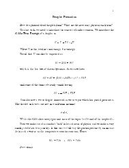
How then can we understand the existence of the weak decay
8
5B → 8 4Be + e + + ν e ,
which requires the p → n process? The point here is that the binding energies
of the B and Be nuclei are different. In this case the 8 4Be nuclei is more
tightly bound (larger binding energy E b ) than the 8 5B by an amount larger
than the difference between p and n plus e + rest energies, making the process
energetically possible. Figure 1 shows the binding energy per nucleon for all
isotopes as a function of atomic mass A. We see that the maximally bound
nuclei are in the vicinity of iron (Fe).
1.4 A process which gives hydrogen burning
We assume initially that the main sequence star under consideration consists
entirely of hydrogen, or at least the presence of other elements can be ignored.
As we have seen, a typical temperature in the core of a MS star like the sun
is T ≈ 10 7 K. The average kinetic energy of the constituents of a classical
gas is
E = 3 kT ≈ 1 KeV (1)
2
for T = 10 7 . Since this energy is much larger than the atomic binding energy
of the hydrogen atom, the hydrogen is completely ionized. Hence the core is
a dense gas of positively charged protons and negatively charged electrons.
We need to find a way for the protons to interact and fuse to form heavier
elements. As Figure 1 shows, the creation of heavier elements (up to iron)
will allow the binding energy of the product to be released as kinetic energy,
thus providing the stellar energy source.
4

Figure 1: Binding energy per nucleon in MeV as a function of atomic mass
A. (Figure 10.9 of Carroll and Ostlie.)
The most obvious potential candidate is p + p → 2 2 He. However, this
state does not exist in nature — there is no proton-proton bound state.
We next consider the process which actually does take place, and is the
first step for all stellar hydrogen burning:
or in nuclear notation:
p + p → d + e + + ¯ν e (2)
1
1H + 1 1H → 2 1H + e + + ¯ν e (3)
where d = 2 1H is the deuteron. We see that this process involves the (inverse)
β decay process mentioned earlier: p → n + e + + ¯ν e , where the resulting neutron
forms the deuteron bound state with the surviving proton. So although
the positive energy for this process results from the d binding energy due to
the strong force interaction of n-p, this initial step utilizes the weak force.
This is important, since, as we shall see below, the low rate for this weak
process guarantees a long life for MS stars. Before we consider the reaction 3
and the remainder of the proton-burning sequence in more detail, we consider
a simple model of the n-p bound state, the deuteron.
5

1.5 A simple model of the deuteron
An approximate form of the strong force for nucleons is the square well
potential energy shown in Figure 2. The radius of the well of approximately
r 0 = 2 fm and its depth of 36 MeV are based on the results of scattering
experiments. When the Schrodinger equation is applied to this system with
the n and p masses, one finds that only one bound state results with an
energy eigenvalue of −2.2 MeV. This indeed correspnds to the experimental
finding that the deuteron consists of only one bound state with a binding
energy of 2.2 MeV.
U(r)
(MeV)
-2.2
r o
r
-36
Figure 2: Square well model of the deuteron.
6

2 Stellar Energy Generation – PP-chain physics
2.1 The PPI chain and energetics
Figure 3 shows the main sequences by which hydrogen nuclei (protons) are
converted into helium nuclei. The first step is the weak interaction process
of Eq. 3. This step determines the rate of energy production in MS stars,
and this property is the focus of the next two sections. Here, we look at the
overall energetics of the processes.
Figure 3: The PP chains. (Figure 10.8 of Carroll and Ostlie.)
All three of the PP chains involve conversion of 4 protons to a helium-4
nucleus. Reference to 1 shows that 4 2He is unusually stable relative to isotopes
of similar atomic mass. In fact, 4 2He is also known as an alpha particle, and
due to its large binding energy and stability, is a typical by-product of nuclear
reactions such as fission. Figure 3 shows a branching ratio of 69% for process
3 of the PPI chain. This reflects the probability of this path. However, the
PPI chain accounts for 85% of the overall rate of 4 2He production, and hence
about 85% of the total energy output of the sun and similar MS stars. So we
use the PPI chain to illustrate energy production, and in so doing we account
7

for the vast majority of the solar luminosity.
Rewriting the PPI chain:
1
1H + 1 1H → 2 1H + e + + ν e
2
1H + 2 1H → 3 2He + γ
3
2He + 3 2He → 4 2He + 2 1 1H (4)
We note that process 3 requires two reactions each of processes 1 and 2. So
in sum there are 6 protons reactants and 2 proton products. Hence, the net
effect of the PPI chain in terms of overall energetics is equivalent to:
4 1 1H → 4 2He + 2e + + 2ν e + 2γ . (5)
We follow the usual practice in nuclear physics of using the atomic mass
unit, or u for the rest masses of nuclei. By definition,
1u = 1 12 M(12 6 C) ,
and a conversion to MeV can be made from Section 1.2. Using the AMU,
the proton mass is 1.0078 u and the 4 2He mass is 4.0026 u. So the energy
available to the other final state particles, both as rest energy and kinetic
energy, is
∆m = [4 × 1.0078 − 4.0026] = 0.0287 u ,
or ∆mc 2 = 0.0287×931.49432 MeV/u = 27 MeV. The positron rest mass will
be available for kinetic energy, too, since it will annihilate with an ambient
electron. So except for the energy given to the neutrinos, which exit the star
without depositing any energy, the 27 MeV is available to provide the solar
luminosity. (The neutrinos will be discussed separately in lecture 6.) We
note that the first step of the PP chain, the p-p interaction, provides only
about 0.3 MeV of kinetic energy.
So for each PPI reaction (i.e. for every 4 protons), the fraction of stellar
mass which is converted to energy luminosity is (except for the neutrinos)
ɛ = 0.0287/4.0313 ≈ 7 × 10 −3 (6)
Hence, the available hydrogen mass can be eventually converted into energy
with an efficiency of 0.7%.
8

2.2 The pp interaction: Coulomb barrier penetration
The strong force for the n-p and p-p interactions are identical. (This is a
symmetry property called isospin.) But we now have to add to this the
Coulomb interaction between the protons:
U(r) = U strong + U coulomb , U coulomb = 1 e 2
4πɛ 0 r
This potential is depicted in Figure 4.
(SI)
U(r)
(MeV)
0.7
E
r o
r
Figure 4: Potential energy model of the proton-proton interaction.
At r = r 0 = 2 fm we have (using SI units, then converting to eV):
U coul = [ (9 × 10 9 )(1.6 × 10 −19 ) 2 /(2 × 10 −15 ) ] ×1 eV/1.6×10 −19 J = 0.7 MeV
So while the Coulomb barrier is 0.7 MeV, the average kinetic energy of the
protons, from Equation 1 is ≈ 1 KeV. So classically, a proton at this average
energy will never be able to get close enough to another proton to engage
in strong or weak interactions. However, quantum mechanics provides the
possibility of barrier penetration. We now sketch the solution to this calculation,
which will be familiar to students who have had an introductory
quantum course.
9

In the case of a 1-dimensional step potential of height U b and width L, a
particle of mass m and kinetic energy E has a barrier penetration probability
P G in the case where E ≪ U b of P G ≈ e −γ , where γ 2 = 8mL(U b − E)/¯h 2 .
For our potential of Fig. 4, where we assume spherical symmetry, we have
an analogous solution to the 1-dimensional step potential, except that we
now have to integrate over the Coulomb potential. So U b is replaced by
a geometrical factor multiplied by the barrier height. In the limit E ≪
0.7 MeV, which is our situation, the solution for the barrier penetration
probability becomes
P G dE ≈ e −γ dE , γ 2 = E G /E , (7)
where E G , known as the Gamow energy, depends on the composition of the
charged-particle gas. In the present case for protons, this is
E G = (2µ m /¯h 2 )
[ e
2
4ɛ 0
] 2
(8)
in SI units, where µ m is the classical reduced mass of the p-p system, m p /2.
The factor 1/4 comes from the integral over the Coulomb barrier. Using
combinations defined in Section 1.2 gives
E G = 1 m p c 2
( ) π 2
8 ¯h 2 c 2 (4π¯hcα)2 = (938 MeV) = 0.49 MeV
137
Therefore, for an average proton kinetic energy of 3 kT = 1 KeV, we find
2
the Coulomb barrier penetration probability to be
P G ≈ e − √490/1 ≈ 10 −10 (9)
One can compare the probability above with that for which the protons
exceed the classical Coulomb barrier because there is a small fraction which
have thermal energies far above the average. For a classical, non-interacting
gas the distribution of kinetic energies at a temperature T is given by the
Maxwell-Boltzmann distribution:
P mb (E)dE ∝ E 1/2 e −E/kT dE (10)
which follows the exponential decay form far above the average. For kT ≈ 1
KeV, the probability of finding a proton at the Coulomb barrier is ∝ e −720
10

compared to the quantum barrier penetration factor which we found to be
∝ e −22 . Clearly the thermal mechanism is insignificant compared to quantum
tunneling in this case.
A correct determination of the probablility of Coulomb barrier penetration
should involve the convolution of the two distributions, of the form:
P G (E) =
∫ ∞
0
P q (E ′ )P mb (E − E ′ )dE ′ (11)
The resulting distribution, called the Gamow curve, has a maximum at about
5 KeV for a star like our sun.
2.3 Proton survival time
We can now estimate the rate of the initial hydrogen-burning process given
in Equation 3. As stated earlier, this process is the slowest in the PP chain,
and hence determines the rate of energy production in main-sequence stars.
This rate is given by
R pp = R col P G P pn (12)
where R col is the pp collison rate, P G is the barrier penetration probability
of Equation 11, and P np is the probability that a barrier penetration results
in the weak process p → n + e + + ν.
In class, we estimated the collision rate using the standard formulation
R col = nvσ, where n is the number density of protons, v is their average speed,
and σ is the collision cross section. n is about 10 26 cm −3 . We can find v from
3
2 kT = 1 2 mv2 = Ē ≈ 1 KeV, which gives (v/c)2 = 2Ē/(mc2 ) = 2/9.38 × 10 5 ,
so v ≈ 4 × 10 7 cm/s. And we find σ from the proton scattering radius (∼ 1
fm, giving σ ∼ 10 −26 cm 2 . So then we have
R col ≈ (10 26 )(4 × 10 7 )(10 −26 ) ∼ 4 × 10 7 s −1
Because the weak force has such a short range, its strength is very small
relative to the strong force for the rather large deBroglie wavelengths (λ =
h/p) associated with the 1 KeV protons in the stellar cores. Therefore, even
after a proton manages to penetrate the Coulomb barrier of the other proton,
it is very unlikely that the weak process we need will occur rather than p-p
elastic scattering via the strong interaction. Hence, we need to estimate
P pn = P (p → n + e + + ν)/P (pp → pp)
11

. We are now going to revise and reformulate the expression in Equation
12 compared to what was done in class in order to fill in the pieces more
easily. We note that since the collision is dominated by strong p-p scattering
at these energies, then P pp ≈ P col . Furthermore, P pn = Γ pn /Γ pp , where Γ
is the transition rate (transition probability per unit time). Hence, we can
re-write Eq. 12 as
R pp = R col P G P pn = NΓ pp P G (Γ pn /Γ pp ) = NP G Γ np (13)
where N is the number of protons available for the pp process. Now the rate
for the weak β decay process can be used to evaulate Γ np . It is a standard
nuclear/particle calculation (see for example Halzen and Martin (1984)):
Γ = G2 ∫ E0
p 2 (E
¯hπ 3 0 − E) 2 dp , (14)
0
where p and E = √ p 2 + m 2 e are the daughter electron’s momentum and energy
(c ≡ 1 momentarily), and E 0 is the binding energy difference between
final and initial nuclei. (This calculation ignores many details, but should
provide an order of magnitude estimate.) G is the Fermi (or weak) constant,
which is related to the strength of the weak force: G/(¯hc) 3 = 1.2 × 10 −5
GeV −2 . An evaluation of the integral in the expression above is shown in
Figure 5 as a function of E 0 . The relativistic approximation p ≫ m e c often
shown in texts is clearly not appropriate for binding energies of the p-p reaction.
Using E 0 = 0.3 MeV for the p-p process, Eq. 14 yields Γ ∼ 10 −7 s −1 .
Combining this with the Coulomb barrier penetration probability Eq. 9, we
find
R pp ∼ (N)(10 −17 ) s −1
Therefore, our order of magnitude calculation yields an average lifetime
for protons in the core of solar-like MS stars of
τ p = N/R pp ∼ 10 17 s
or about 10 billion years, which is the appropriate time scale. Along with
the overall energy output for the PPI chain found in the previous section, we
now have a viable model for MS star energy generation.
12

0.01
0.009
0.008
0.007
0.006
I (MeV 4 )
0.005
0.004
0.003
0.002
0.001
0
0.1 0.2 0.3 0.4 0.5 0.6 0.7 0.8 0.9 1
E o (MeV )
Figure 5: The integral in Eq 14 as a function of E 0 .
2.4 Other nuclear sequences
As discussed in Carroll and Ostlie, the temperature dependence of the PP
chains is roughly given by R pp = α pp (T/10 6 ) 4 , where α depends on many
other parameters. Other nuclear fusion processes are also possible. One
example is the CNO cycle, depicted in Fig. 6.
Typically, these processes involve heavier nuclei, and the temperature dependence
is much greater than the PP chain. For example, R cno = α cno (T/10 6 ) 20 .
Two other chains, with even greater temperature dependence, are depicted
in Figs. 7 and 8. The latter only becomes relevant for T ∼ 10 9 K. The basic
scenario for how these other chains come into play is as follows. For solar-like
MS stars with a core temperature ∼ 10 7 K. At this temperature, the PP rate
dominates the rate, as expected. The higher-A processes have much lower
rate at these temperatures, so represent a small correction to energy and element
production. Now, since the equation of state gives a pressure P ∝ T ,
in the steady state of hydrogen burning the PP will continue to dominate.
13

Figure 6: The main branch CNO chain.
Ostlie.)
(Equation 10.51 of Carroll and
However, as hydrogen is depleted the PP pressure is reduced, allowing further
gravitational contraction, in turn requiring larger pressure to maintain mechanical
equilibrium with a correspondingly larger T . The larger T rapidly
increases the rate of the higher-A processes. So as the lighter nuclei are consumed,
the burning of these elements will continue at layers ar larger radius,
while the inner core will involve the processes with heavier nuclei. These
larger rates will consume the fuels relatively quickly. At some point in this
evolution, electron degeneracy becomes important. This will be discussed in
subsequent lectures.
Figure 7: Another high-temperature fusion process. (Equation 10.59 of Carroll
and Ostlie.)
14

Figure 8: Yet another high-temperature fusion process. (Equation 10.60 of
Carroll and Ostlie.)
15

3 Solar neutrino physics
Nuclear processes in stellar cores produce large numbers of neutrinos of energy
∼ 1 MeV. The feeble interaction of neutrinos with matter ensures that
they exit the core and star with near 100% transmission. This makes neutrinos
a unique probe of stellar astrophysics. Here we focus on MS stars,
specifically the sun. The underlying physics, the story of solar neutrino
detection, and the “solar neutrino problem,” and its resolution are briefly
discussed in this lecture.
3.1 Neutrinos are elementary particles
We discussed neutrinos earlier in our brief introduction to the elementary
particles. Because the neutrinos couple only to the weak force, they are very
difficult to detect directly. It is not so much that the weak force has a small
intrinsic strength — the coupling constant is actually slightly larger than the
electromagnetic coupling. The weak force, however, has a very short range.
So while at an energy ∼ 100 GeV, the strength is comparable to EM, at
low energy, where the deBroglie wavelength is large compared to the force
range, the effective strength is tiny. The range helps us understand why the
primary neutrino cross sections obey σ ∝ E 2 for E ≪ 100 GeV, which is the
range of interest for us.
A neutrino interaction was not directly observed until 1956 by Reines and
Cowan. However, their existence was inferred and expected beforehand. In
1932 Pauli predicted their existence. He based this on the observed energy
spectra of electrons or positrons from beta decay processes such as
8
5B → 8 4Be + e + [+ν e ] .
If the final state really consisted only of 2 bodies, then E e is a constant,
depending only on the masses involved. Instead, a continuous distribution
was observed for E e . Pauli reasoned that either energy is not conserved in
such decays (!) or an undetected particle was present in the final state. . . the
neutrino.
There are 3 species of neutrinos, ν e , ν µ and ν τ , one in each of the 3
“generations” of elementary particles. However, with notable exceptions,
most processes we consider in astrophysics involve only generation 1 (this is
the lightest), so we mostly encounter ν e (and ¯ν e ). Neutrinos were originally
assumed to be massless. However we now know their masses to be finite, in
16

part due to the solar neutrinos discussed below. Their mass values are not
known, but they are small, likely to have m ν ≪ 1 eV/c 2 .
3.2 Predictions for neutrino production
A simple calculation provides a good estimate of the expected flux of solar
neutrinos at the earth. By first approximation, the PPI chain provides the
solar power we observe on earth. As discussed in lectures 4 and 5, every
iteration of this sequence results in 2 ν e and 27 MeV of kinetic energy, which
we observe eventually as luminosity. This luminosity corresponds to a power
of 137 mW/cm 2 = 8.53 × 10 11 MeV/(cm 2 s. Hence, we expect the neutrino
flux at earth to be
8.53 × 10 11 /(27/2) = 6.4 × 10 10 ν e ′ s/(cm 2 s) .
Figure 9 is the state of the art prediction of the overall solar neutrino
flux at earth from Bahcall, et al. The estimate above is indeed rather close
to the calculated PP flux. The peaking of the curves near the maximum
energy is due to the parity-violating nature of the weak interaction. We note
that although the PP neutrinos dominate the flux, their energy is limited to
below ≈ 0.4 MeV. The neutrinos from 8 5B decay on the other hand extend
to about 15 MeV.
3.3 Solar neutrino detection
Detection of neutrinos in general is difficult. In high-energy (i.e. elementary
particle) physics, neutrino beams can be produced and used as a very incisive
probe of the weak force. However, this is only practical because the interaction
probability (cross section) inreases rapidly with energy, as noted earlier.
Hence, for a neutrino in a beam with energy ∼ 100 GeV, the interaction rate
is large enough so that an experiment at Fermilab called NuTeV was able
to collect a few million neutrino events over about a year of data collection.
(These were the pictures I showed in class of a huge “splat” of energy in
the center of large quantity of iron.) The experimentalist hoping to measure
solar neutrinos does not have the advantage of such high energy, although
the flux of neutrinos is large, as seen above.
Figure 10 summarizes the principal detectors used to measure solar neutrinos
over the last few decades. The field was pioneered by R. Davis, who
17

Figure 9: Predicted solar neutrino spectra – the flux at earth as a function
of neutrino energy. (From Bahcall.)
18

came up with a viable detector consisting of a large vat of cleaning fluid deep
underground (in a mine at Homestake, SD). The experiment is sensitive to
neutrinos in the reaction
ν e + 37 Cl → e + 37 Ar .
The resulting argon gas bubbles out and is extracted. Since this isotope of
argon is unstable, its quantity is determined by measuring the decay curve.
All solar neutrino experiments are deep underground, so that cosmic ray
particles are filtered out by the overburden. The Davis experiment ran for
about two decades with a measured flux which on average was (34 ± 3)% of
the predicted flux before the result was confirmed by other experiments. In
the meantime, there was a great deal of debate about the result. Davis’s experiment
was primarily sensitive to 8 B neutrinos, since its threshold is above
the PP neutrinos. Could the solar theory be trusted for non-PP sequences,
where there are such large temperature dependences (see lecture 5)? The discrepancy
between theory and experiment was known as the solar neutrino
problem.
Figure 10: Main solar neutrino detectors and measured fluxes. (From
Perkins.)
The next big breakthrough was the gallium experiments, SAGE and
GNO. The technique was similar to the Davis experiment, except using gallium
as the target, which has a threshold of only 0.2 MeV in the process
indicated in Fig. 10. These experiments were sensitive to the PP neutrinos,
and their detected flux was roughly half that expected by theory. Meanwhile,
19

the Super-K experiment in Japan had also confirmed the missing high-energy
flux using a technique which allowed them to actually image the direction of
the neutrinos, confirming their solar origin. The detectors using water as a
neutrino target rely on the following principle. The solar neutrinos collide
with an atomic electron, sending it out into the water as a free particle with
a speed close to c. This is faster than the speed of light in the water, which
has speed c/n, where n is the index of refraction. This results in a shockwave
phenomenom known as Cherenkov radiation, which can be detected by
sensitive light detectors (photo-multiplier tubes) installed on the periphery
of the water tank.
The “problem” was finally resolved a few years ago by the SNO experiment.
Recall that we know that there are 3 species of neutrino, ν e , ν µ ,
and ν τ . The Davis and gallium experiments could only measure the ν e type.
Since only ν e are produced in the nuclear reactions in the sun, this may not
seem to be an issue. However, we note that the Super-K measurements were
slightly sensitive to the other two types, and they measured a higher rate.
The SNO breakthrough was that its detection target material is heavy water,
that is H 2 O where the H is largely deuterium, 2 1H. As we said in lecture 4,
the deuteron is very weakly bound. Hence a neutrino of a few MeV energy
can disassociate the deuteron. The resulting charged proton can be observed
by the Cherenkov technique. This process,
ν x + 2 H → p + n + ν x ,
is equally likely for any of the 3 neutrino species, x.
The SNO result for this reaction is consistent with the predicted solar flux.
This means that the “problem” was not a problem with the solar theory, but
rather indicated a new property of the neutrinos themselves, as discussed
briefly below. The ν e type produced in the solar core were turning into the
other species with some probability on their journey to the earth. The other
detectors only saw the remaining ν e ’s, but SNO saw them all. Hence, SNO
not only confirmed the origin of the “problem,” but also confirmed that the
solar theory indeed predicted the correct neutrino flux. Davis shared the
2002 Nobel Prize in physics.
3.4 Neutrino oscillations and mass
To illustrate the point, we discuss only two neutrino species. The generalization
to three is qualitatively the same, but is more complicated. Let the
20

neutrino species have small, but finite masses, with values (eigenstates) m 1
and m 2 . The quantum state for m 1 will in general be a linear combination
of ν e and ν µ . The state begins as ν e , as determined by the weak interaction
process in the solar core. Now, quantum mechanics requires that the mixed
state evolve in time according to
ψ(t) = ψ(0)e −ı(∆E) t/¯h ,
where ∆E is the energy difference of the states. Relating this to the mass
eigenstates and t to the distance travelled, the probability for transition from
one type of neutrino to the other, called neutrino oscillation, over a distance
L (in km) in vacuum becomes:
P 1→2 = P 2→1 = sin 2 (2θ) sin 2 ( 1.27∆m 2 L/E ) (15)
at an energy E (in GeV), and ∆m 2 = m 2 2 − m 2 1 is in eV 2 /c 2 . The parameter
θ determines the linear combination ψ 1 = cos θ ψ e + sin θ ψ µ and is called
the mixing parameter. One additional detail: While the neutrinos do not get
significantly absorbed by the sun on their outward trek, there is an interesting
resonance effect where the neutrino mass difference matches the ambient mass
density. The interaction is analogous to light passing through transparent
material with index of refraction > 1. The effect is called MSW enhanced
oscillations, and can easily result in maximal mixing of the neutrino states,
i.e. tan θ ≈ 1. In this case we would also expect the ratio of ν e to total flux
at earth to be ≈ 1 , with some energy dependence from Equation 15. The
2
data are consistent with both of these predictions.
Hence, the resolution of the solar neutrino problem requires finite neutrino
masses. This effect has also been seen in other types of neutrino experiments,
so it is known that all 3 types mix with each other. While only ∆m 2 is
directly measured, the implications from all the data are quite strong that
the individual masses are very small, m ≪ 1 eV/c 2 . If this is indeed the case,
as we shall see later, this makes neutrino mass irrelevant for cosmology.
21

4 Type II Supernova Physics
We consider the physics and phenomenology of supernovae, energetic explosions
of stars, focussing on the so-called Type II type of supernova, which
involves an evolved, massive star which is not necessarily a member of a binary
system. As discussed in the next lecture, a supernova event produces
a shock wave of rapidly expelled stellar material which is bombarded by a
huge neutron flux. Neutron capture events result, leading to the production
of elements heavier than iron and nickel, which we haven’t been able to
produce in the stellar processes discussed so far. Hence, heavy elements are
produced exclusively by supernovae, and the development of earth and its
life forms depend on at least one cycle of heavy star evolution and subsequent
supernovae.
4.1 Massive star core collapse sequence
Consider an “evolved” star, one which has evolved off the main sequence and
has an evolved mass M which may be significantly smaller than its zero-age
main-sequence (ZAMS) mass. As discussed in previous lectures, at some
point the pressure due to electron degeneracy becomes important. This is
the pressure which results from electrons being forced to higher-energy states
due to the Pauli exclusion principle, which applies to all fermions (spin= 1 2¯h
particles), such as electrons or neutrons. Now if M < 1.4M ⊙ , then the
electron gas is non-relativistic, and the electron pressure is ∝ n 5/3 , where
n is the electron number density, and the star is stable under gravitational
collapse, since the gravitational pressure is ∝ n 4/3 . The fate of such a star
is a white dwarf, as discussed before. The mass 1.4M ⊙ is known as the
Chandrasekhar mass.
However, if the evolved mass is > 1.4M ⊙ , then the electron gas is relativistic,
the electron pressure is ∝ n 4/3 , and the star is in unstable equilibrium
with the gravitational pressure. Eventually, an unstable equilibrium always
moves toward a stable equilibrium at with lower potential energy configuration.
A massive, evolved star would eventually have a core temperature of
∼ 5 × 10 9 K and a density of ∼ 3 × 10 10 kg/m 3 . The average thermal kinetic
energy of nucleons is then ∼ 1 MeV and the Boltzmann distribution extends
to sufficiently high energy to allow fusion of nuclei up to nickel and iron (see
Figure 1 from Lecture 4). After iron, it is energetically unfavorable to go to
higher atomic number, so the massive star develops an iron core with silicon
22

urning in the next sub-shell outward in radius. The silicon eventually ends
up as iron, too, but after about one day this fuel is exhausted. Our massive
star is now in unstable mechanical equilibrium, supported only by the
electron degeneracy pressure.
The following describes what is thought to be a typical sequence of events
for the collapse of a massive star, resulting in a supernova event. However,
keep in mind that rotation and magnetic fields, which we have ignored so
far, may have an important role, although the outcome is unlikely to change
significantly.
1. After fusion processes fizzle out, there is some gravitational collapse
which causes heating to T ∼ 10 10 K. This is sufficient to trigger two
processes:
(i) Photo-disintegration of iron and the subsequent photo-disintegration
of the products, eventually leading to complete “inverse fusion,”
with products p and n:
γ + 56 Fe ↔ . . . → 13 4 He + 4n ; γ + 4 He → 2p + 2n (16)
(ii) Inverse beta decay. When electrons have K > 3.7 MeV then the
following can occur:
e − + 56 Fe → 56 Mn + ν e
and by time we get down to nucleons:
e − + p → n + ν e (17)
Note that the Fermi energy of the degenerate electron gas is ≈ 4
MeV at a density of 10 12 kg/m 3 , so there are plenty of electrons
which can trigger these inverse beta decays.
2. The processes above are endothermic, that is they remove kinetic energy
(and hence fluid pressure) from the core. The unstable core now
quickly collapses.
3. The iron core is now in free fall. The time of fall to a much smaller
equilibrium radius is ∼ 100 ms.
23

4. During collapse, the neutronization processes in Eqs. 16 and 17 proceed
rapidly. Neutrinos result as well, and these mostly exit the star. This
neutrino emission represents about 1% to 10% of the total emission,
the remainder resulting from subsequent steps.
5. The collapse ends when the core reaches nuclear density. Actually, the
density exceeds nuclear briefly by what is estimated to be a factor of 2
to 3. This is discussed with some more detail in Section 4.3 below.
6. The core now strongly bounces back to nuclear density from the supernuclear
density. We can think of the protons and neutrons as bags of
quarks bound together by very strong springs (spring constant ∼ 10
GeV/fm 2 ) which are compressed by the collapse, but then spring back
to equilibrium, thus the bounce.
7. The bounce sends a shock wave outward at high velocity, blowing off
the remaining stellar atmosphere in the process. One the shock reaches
the outer atmosphere, the photons emitted by recombination, powered
by the shock itself and by subsequent nuclear decays, become the visible
supernova explosion.
8. The core will radiate away its huge energy content in neutrinos, as
discussed below, and the remnant core will settle down into a neutron
star. The radius is something like 15 km, depending on initial core
mass, but has a mass of 1.4 to about 3 M ⊙ .
9. The neutron-rich shock, meanwhile, will induce creation of elements
heavier than iron by neutron capture. This will be discussed in the
next lecture in more detail.
10. The shock continues into interstellar space at speeds of ∼ c/10. For
example, the crab neubula, resulting from the 1054 A.D. supernova is
large and still expanding.
11. The neutron star may become visible in radio as a pulsar, depending on
rotation and magnetic fields. The crab’s neutron star is indeed a very
“loud” pulsar, faithfully producing a radio burst once per revolution,
every 33.3 ms.
The visible-light luminosity of a typical supernova is roughly 10 42 J, with a
peak power of 10 36 J/s = 10 36 W. This is about a factor 10 10 greater than the
24

solar luminosity, which is comparable to an entire galaxy. The visible light
decays exponentially as unstable nuclei decay, so the supernova is visible for
weeks, depending on its location. This is discussed more in the next lecture.
However, as impressive as the light output is, it represents only about 1%
of the total energy output, as we shall see in Section 4.4. We follow up now
with some detail.
4.2 Energy from collapse
We saw earlier that the total gravitational energy released in collapse is the
change in potential energy given by
E grav = 3 GM 2
5 R
when the final radius R is much smaller than the initial. (In our case, the
ratio is ∼ 10 −3 .) Using M = 1.5M ⊙ , that is, just over the Chandrasekhar
limit, then with R = 15 km we get
E grav = 6 × 10 46 J = 4 × 10 59 MeV (18)
This is a big number! It will feed into the energy release of the supernova.
4.3 A very large nucleus
As mentioned above, the collapse proceeds to nuclear density, where it is
halted by the strong nulcear force. It takes collision energies of ∼ 10 GeV to
partially break up a nucleon (neutron or proton). As we shall see momentarily,
the average energy from the collapse is still 2 orders of magnitude from
this. So the nucleons, predominantly neutrons at this point, get squeezed by
the collapse to sub-nuclear volume, then rebound, giving rise to the supernova
bounce and the return to nuclear density.
So we are justified in treating the collapsed core as closely packed nucleons,
essentially at nuclear density, and consisting primarily of neutrons. As
we saw with the electrons, the neutrons will also form a degenerate “gas”
since they are fermions. We return to this briefly at the end. In any case,
the collapsed core will settle down into what is termed a neutron star.
Nuclear density ρ N we can estimate by the average density of a proton
(or neutron):
ρ N = m p /(4πr 3 o/3) = 2 × 10 17 kg/m 3 ,
25

where we have used r o = 1.2 fm for the proton radius, based on lab scattering
measurements. With ρ N as the average nuclear density, then the total mass
of this proto-neutron star is
M ns = Nm p = ρ N 4πR 3 /3 ,
where N is the total number of nucleons (neutrons). Combining these, and
using M ns = 1.5M ⊙ yields:
R = r o N 1/3 = 15 km ; N = 1.5M ⊙ /m p = 2 × 10 57 . (19)
Combining Eqs. 19 and 18 gives an estimate for the average energy per
nucleon of (3 × 10 59 /(2 × 10 57 ) ≈ 100 MeV/nucleon. This number provides
two lessons:
• It is a large kinetic energy, but far short of what is required to break
up the nucleons.
• Recall from Fig. 1 of Lecture 4 that iron had the largest binding
energy per nucleon at 8 MeV/nucleon. The collapse provides more
than enough energy to completely break up even iron into constituent
nucleons, as we had presupposed.
4.4 The first seconds of the proto-neutron star
Because the proto-neutron star is so dense, a qualitatively new feature is
manifest. Namely, the vast majority of the collapse energy of Eq. 18 can
not easily escape. To see this, we calculate the mean free path of the most
weakly interacting particles, the neutrinos.
As we saw in Lectures 5 and 6, the collision rate is given by nσv, where
n is the number density and σ is the interaction cross section. Hence, the
time between collisions is the inverse of this; and the mean distance between
collisions (the mean free path) is l = v/(nσv) = 1/(σv). In this case,
n = N/(4πR 3 /3) and σ is the neutrino-nucleon cross section. The so-called
charged-current cross section for the process n + ν e → p + e − is given by
σ cc = 5.8
( ) E 2
π G2 F E 2 ≈ 10 −45 m 2 ,
1 MeV
where G F is the weak (Fermi) coupling constant encountered in Lecture 5. If
we use E ν = 20 MeV, this gives l ≈ 2 m ! The mean free path for neutrinos
attempting to escape the collapsed core is only a few meters.
26

As it turns out, the neutral current scattering process ν x + n → ν x + n
is also possible here, where x represents any of the 3 neutrino species. A
similar calculation (a bit more complicated) for this process gives l ≈ 10 m.
Hence we arrive at the following conclusions:
• The collapse energy is locked in the proto-neutron star and can only be
carried away by neutrinos. Estimates are that about 99% of the total
energy of collapse is carried by the neutrinos.
• The neutrinos are radiated from a thin few meter thick skin on the
outside of the core.
• With l ∼ 10 m, the energy transport via neutrinos is a random walk,
diffusion problem. We can estimate the diffusion time to be t ∼
R 2 /(cl) ∼ 1 s. This compares to a speed of light flight time of ∼
R/c ∼ 10 −4 s.
• There are effectively 6 neutrino populations in thermal equilibrium with
the super-hot core – 3 species, with both neutrinos and anti-neutrinos.
These all share the energy transport via the neutral current process.
Hence we expect the 150 MeV/nucleon to be carried away with an
average energy per neutrino of 150/6 ≈ 20 MeV.
Thus, along with the visible supernova, we expect a huge neutrino flux
equal to the collapse energy ∼ 10 59 MeV carried by about 10 58 neutrinos in
all 3 species and ν plus ¯ν with average energy 20 MeV.
4.5 SN1987a
In 1987 supernova was observed at earth located in the large magellenic
cloud (LMC), a small galaxy adjacent to the milky way, at a distance of
about 60 kpc. Luckily, two underground proton decay experiments were
taking data. These detectors can observe neutrino events using the water
technique discussed in Lecture 7a. (In fact, one of the detectors, Kamiokande,
later became the Super-K detector encountered in 7a.) The two detectors
simultaneously observed a burst of neutrino events about 7 hours before the
optical supernova was observable. The predominant detection process was
¯ν e + p → n + e + .
27

Figure 11: Neutrinos detected from SN1987a with the IMB and Kamiokande
detectors.
The neutrino data is reproduced in Fig. 11.
We can now compare the observations with our expectations. The measured
neutrino energy is indeed about 20 MeV. (The apparent decline with
time can be used to determine neutrino mass. The limit turns out to not
be better than terrestial experiments.) The neutrinos are indeed spread out
in time by ∼ 1 s. (Again, finite neutrino mass can disperse this somewhat.)
The number of detected events was 20. Only ¯ν e were observed, so the total
flux at earth was 20 × 6/σ d ≈ 10 10 /cm 2 , where σ d is the detection cross section
times efficiency. Translating this flux to the distance of the LMC gives a
total energy of 2 × 10 59 MeV, in good agreement with our expectations from
the previous section.
It is interesting to note that the neutrino burst from the collapse may
in fact transfer enough energy to the supernova shock front to keep it from
falling back onto the collapsed core. This may, in fact, require all 3 neutrino
species (although the calculations are difficult), in which case we would
require the 3 species to make heavy elements (and life on earth).
28

4.6 Further collapse and black holes
We discussed collapse stoppage and bounce above in terms of the strong
nuclear force. However, since we form a core of mostly neutrons, we might
expect neutron degeneracy to also play a role. And it does. As the protoneutron
star radiates away its collapse energy we might expect it to undergo
further collapse if not for the degeneracy pressure. Carrying out the same
calculation we did earlier for electrons results in an equivalent Chandrasekhar
mass of about 5.6M ⊙ . If the collapsing core mass exceeds this, then we might
expect the collapse to proceed to a black hole. If less, then it remains a
neutron star.
However, the observed transition from neutron star to black hole is closer
to 3M ⊙ . We might have expected that this would not be so simple. Among
the complicating factors, all difficult to calculate, but important in this
regime, are:
• repulsion due to the strong nuclear force
• neutron degeneracy
• non-linear gravity; that is, strong gravitational effects, as predicted by
General Relativity
• large angular velocity
• large magnetic fields
On the note of strong gravity, we finish by mentioning the Schwarzschild
radius, R s , predicted by GR as the “event horizon” where proper time intervals
go to zero and light cannot escape. It is given by
R s = 2GM/c 2 .
For M = 5M ⊙ , R s ≈ 15 km, comparable to the size of our neutron star,
but with larger mass. Adding mass to a neutron star would result in a black
hole. If the initial collapsing core had mass ∼ 5M ⊙ or more, the collapse
might proceed directly to a black hole, although many researchers believe
there would be a stopping bounce followed by infall back onto the collapsed
core, leading then to a black hole.
29

5 Cosmological expansion
In this lecture we discuss Hubble’s observation of galactic redshifts in the
context of general relativity. The cosmological principle provides simplifying
assumptions, allowing to an “equation of motion” for the scale factor R
known as the Friedmann equation. This equation will be a starting point for
many of our discussion of physics of the early universe.
5.1 Spacetime in Relativity
In special relativity, a key concept is the invariant spacetime interval ds 2 :
ds 2 = (c dt) 2 − ( dx 2 + dy 2 + dz 2) ,
which separates two points in spacetime. The interval ds is the same for any
observer in an inertial reference frame. It can also be written equivalently as
ds 2 = ∑ g µν dx µ dx ν ,
where g µν is the metric tensor and dx µ = (ct, x, y, z) are 4-vectors. For the
flat spacetime of special relativity, g µν is the Minkowski metric, represented
by a 3 × 3 matrix with diagonal elements 1, −1, −1, −1, and all other
elements zero.
In spherical coordinates, then the interval in flat spacetime becomes:
ds 2 = (c dt) 2 − dr 2 − r 2 ( dθ 2 + sin 2 θdφ 2) .
This can be compared with the Schwarzschild interval which is a solution of
the equations of general relativity for the case of spherical symmetry at a
distance r from a mass M:
ds 2 =
[
1 − 2GM ] [
(c dt) 2 − 1 − 2GM ] −1
− r ( 2 dθ 2 + sin 2 θdφ 2) . (20)
rc 2 rc 2
The proper time dτ measured by a clock at rest at a distance r from the
mass is given by
[
(c dτ) 2 = 1 − 2GM ]
(c dt) 2 ,
rc 2
where dt is the time measured in a distant inertial frame. We see that as
one approaches the distance r = 2GM/c 2 ≡ R s , the proper time interval
30

approaches zero. This distance R s is the Schwarzschild radius encountered
before, representing the horizon of a black hole.
Finally, under the assumptions that the universe is isotropic and homogeneous,
the FLRW interval result for general relativity is
[
ds 2 = (c dt) 2 − R(t) 2 dr 2
]
1 − Kr + 2 r2 dθ 2 + r 2 sin 2 θdφ 2 , (21)
where R(t) is the scale parameter and K represents the type of spacetime
curvature. The equations can be re-scaled so that K conventionally can take
on one of three discrete values:
• K = 0. Flat spacetime. The 2-d analog is a flat sheet.
• K = +1. Positive curvature. The surface of a balloon in 2-d.
• K = −1. Negative curvature. A saddle point in 2-d.
The scale parameter R(t) represents the fractional expansion of the distance
between two points due to cosmological expansion (see next sections).
So if r o is a distance between two objects, then at a later time, the true coordinate
distance between the objects has become r(t) = R(t) r o . (r o is known
as the comoving coordinate distance.) Note that R(t) is only a function of
time.
5.2 Hubble’s Observation and its interpretation
The redshift z measures the fractional shift of the observed wavelength λ ′ of
a spectral feature, e.g. an emission line, relative to the wavelength λ of the
feature measured in a proper frame. So z = ∆λ/λ = (λ ′ − λ)/λ, or
λ ′ = λ(1 + z) (22)
Hubble observed redshifts for tens of relatively nearby galaxies for which
their distance was independently known. The relativistic Doppler shift provides
an explanation for a shift of wavelength due to the motion v of the
source with respect to the observer:
λ ′ /λ =
[ ] 1/2
1 + (v/c)
≈ 1 + v 1 − (v/c) c ,
31

where the approximation is valid only for v ≪ c. Combining this with Eq.
22 gives z ≈ v/c, which Hubble used to then arrive at his hypothesis:
v = H o r .
H is the Hubble parameter, and the subscript refers to its value at our current
epoch. The presently accepted value of H o is about 70 (km/s)/Mpc.
The interpretation of the galactic redshifts in terms of a Doppler shift
fails to be consistent with the data at larger values of z. In addition, it
implies that the Earth (or at least our galaxy) is in a unique position in
the universe. It violates the cosmological principle, that the universe, at
sufficiently large distance scales, is isotropic and homogeneous. Consistency
with this principle implies that spacetime itself is expanding, along with its
contents, and that the expansion was initiated a singular event, the big bang.
As we will see, this hypothesis is consistent with all well-defined predictions
to date, including the redshifts, and has successfully predicted a large number
of diverse observations.
It is natural to describe the cosmological expansion using general relativity.
The scale parameter R introduced above, now becomes the key quantity
used to describe the expansion of spacetime. Two important relations follow
immediately. The scale parameter at a time t after the big bang corresponding
to an observed distant object at redshift z is related to the current scale
R o by
R(t) = R o /(1 + z) . (23)
And Hubble’s hypothesis can be re-written as
Ṙ = HR , (24)
where we have introduced the notation ˙ f = df/dt. We note that if H were a
constant (is is not), then Eq. 24 becomes dr/R = Hdt, which is integrated
to give R(t) ∝ e Ht . In this case, the size of the universe increases by a factor
e in a time
t = 1/H o = 14 Gyr . (25)
This time 1/H o is known as the Hubble time.
Finally, we note that the cosmological principle does not mean that the
universe can not have dramatic structure – in fact, it does – only that such
structure averages out over sufficiently large (i.e. cosmological) distance
scales to look the same in all directions and at all locations.
32

5.3 The Friedmann equation and a useful analog
The field equations of general relativity can be written in tensor form
G µν = 8πGT µν + Λg µν , (26)
where T µν is the stress energy tensor, which contains the description of the
mass and energy densities, G µν is the Einstein tensor, which gives the resulting
spacetime curvature, and Λ is the (infamous) cosmological constant.
We will not use this equation directly, in which many ordinary equations are
embedded.
Envoking the cosmological principle, and assuming matter and radiation
fields can be described as ideal frictionless fluids (more on this part later),
Friedmann found the following solution to Eq. 26 in terms of the scale
parameter R:
(Ṙ ) 2 ( ) 8πG
H 2 = = ρ tot − Kc2
(27)
R 3 R 2
Here, ρ tot is the total energy density and K is the curvature parameter introduced
above.
We can gain significant intuition about the Friedmann equation by showing
its equivalence to a more familiar model. Let us assume that ρ is dominated
by ordinary non-relativistic matter and that this density is uniform.
We put a test mass m at the edge of a sphere of radius R(t). Only the
mass within the sphere, M = 4πR 3 ρ/3, contributes to the gravitational force
acting on m. (This Gauss’s Law for gravity also holds in general relativity.)
Hence, the potential energy of m is −GMm/R, and the total energy
E = E K + U is
1
2 mṘ2 − GMm
R = E .
Substituting M = 4πR 3 ρ/3 and multiplying through by 2/(mR 2 ), then the
left-hand side is identical to Eq. 27. And the right-hand side, the total
energy term, becomes 2E/(mR 2 ). Hence, we can make the identification
E = −Kc 2 /(2m), or
E K + U = E ∝ −K .
5.4 Synopsis of matter-dominated solution
Under our assumption of a matter dominated universe, the analogy presented
above can be related to the familiar classical mechanics problem of a mass
33

subject to a spherically symmetric gravitational field, for which E = 0 represents
the dividing line between m being gravitationally bound or unbound.
So we have:
• K > 0 ⇒ E < 0 ⇒ “bound” (“closed”), R returns to 0.
• K < 0 ⇒ E > 0 ⇒ “unbound” (“open”), R goes to infinity.
• K = 0 (“flat”) ⇒ E = 0 ⇒ R → ∞ and Ṙ → 0 as t → ∞.
These solutions for R(t) as a function of t are summarized in Figure 12.
The last solution, for a flat universe, corresponds in our analog to the solution
for the classical escape velocity, where the velocity of the test mass goes to
zero at infinity. We note that K = 0 is quite strongly favored by current
observations. We also note that in this case, the condition E = 0 means that
two large numbers K and U, the total kinetic and potential energies of the
universe, have to cancel to large precision. We will discuss this seemingly
unlikely situation when we discuss “inflation.”
It is interesting to evaluate the time evolution of the three cases above.
For K = 0, it is easy to show that the Friedmann equation with ρ =
M/(4πR 3 /3) becomes R 1/2 dR = √ 2GM dt, which gives
R ∝ t 2/3
and the age of the universe as 2/(3H o ). Furthermore, the critical density
which enables this E = 0 solution (see homework) can straightforwardly be
shown to be
ρ c = 3H2 o
8πG . (28)
For K > 0, one can show using a similar analysis that a “big crunch”
occurs at a time 2πGM/c 3 ∼ 10 Gyr after the big bang.
34

Figure 12: Time evolution of the scale parameter for the three possible types
of spacetime curvature, K, assuming non-relativistic matter dominates the
energy density.
35

6 Energy densities
We begin with a brief overview of the energy density contributions to the
cosmological evolution of spacetime. Using our definition of the critical density
in Eq. 28, ρ c = 3H2 o
, we can re-write the RHS of the Friedmann equation
8πG
(Eq. 27:
( ) 8πG
H 2 = ρ tot − Kc2
3 R = 2 H2 (ρ/ρ c − 1) − Kc2
R , 2
or
ρ/ρ c = Kc2
R 2 H + 1 . (29)
2
Now, we define
Ω ≡ ρ/ρ c
and we write out the contributions to ρ due to (non-relativistic) matter,
radiation (i.e. relativistic particles), and vacuum energy (see below):
ρ = ρ m + ρ r + ρ v .
Finally, we divide through this expression by ρ c to arrive at
1 = Ω m + Ω r + Ω v + Ω k , (30)
where we have made the definition of an equivalent energy density due to
spacetime curvature:
Ω k = − Kc2
R 2 H 2 .
Current observations of the present epoch give the following best values:
• Ω k ≈ 0 (cosmic µwave background observations, especially the most
recent results from WMAP)
• Ω r ≈ 10 −5
• Ω m ≈ 0.3. All of normal (baryonic) matter is 0.05; the remainder is
dark matter.
• Ω v ≈ 0.7. This would be the contribution due to dark energy – more
on this later.
36

Table 1: Properties of cosmic fluids
R(t) ρ eqn. of state
matter R ∝ t 2/3 ρ ∝ R −3 P = 2 3 ρc2 (v/c) 2
radiation R ∝ t 1/2 ρ ∝ R −4 P = 1 3 ρc2
vacuum R ∝ e αt ρ =const P = −ρc 2
The three types of cosmic fluids which we have input to our general
relativistic description of matter and energy are listed in Table 1, along with
a few of their important properties. The time-dependence t 2/3 for matter was
determined in the previous section.
Figure 15 shows the cooling of the constituents due to cosmic expansion
as a function of time, for the radiation and matter dominated eras. The
transition between the radiation and matter eras occurs at the decoupling
time, t dec ≈ 3 × 10 5 yr ≈ 10 13 s. Before this time, photons, electrons, and
protons were in thermal equilibrium, with
e − + p ↔ H .
At t dec , cooling has gone sufficiently below the ionization energy for hydrogen
(13.6 eV) that the reaction above goes primarily from left to right, thus
producing predominantly neutral matter which is “suddenly” transparent
to photons. These photons are what we currently observe as the cosmic
microwave background (CMBR) with a blackbody temperature of 2.7 K.
This cooling corresponds to a redshift in the wavelength of 1100. So the
decoupling time is:
t dec = 3 × 10 5 yr; (1 + z dec ) = 1100 (31)
This last relation implies that the size of the universe was about 10 3 smaller
at decoupling than today.
Finally, a useful relation is that between R and T :
R ∝ 1/T . (32)
37

Figure 13: Energy (kT ) per particle versus time. Radiation dominated the
energy density until the time of photon decoupling, t dec ≈ 10 13 s.
38

7 Vacuum energy and Inflation
In Section 5 we introduced Einstein’s field equations, Eq. 26, including the
comsological constant (Λ) term. Since g µν represents flat spacetime, this term
is uniformly distributed. For the Friedmann equation, Eq. 27, this term gets
included as Λ/3 on the RHS. Since this term has no R dependence, then for
sufficiently large R, a non-zero Λ will eventually dominate the RHS of Eq.
27. In this case, the Friedmann equation becomes
Ṙ = (Λ/3)R ⇒ dR R = √Λ/3 dt ⇒ R(t) ∝ e αt , (33)
√
where α ≡ Λ/3, as in Table 1.
Now, we make the connection between this funny Λ term in Einstein’s
equations and the idea of vacuum energy from quantum field theory (QFT).
In quantum mechanics, the uncertainty principle states that there can be a
non-conservation of energy ∆E over a time ∆t such that
∆E∆t ≥ ¯h/2 .
In QFT, this must occur with particle pairs such as e + e − appearing and
disappearing, consistent with the uncertainty relation above. On average,
there is a net contribution which is non-zero. This represents the vacuum
energy. So the vacuum is not a state of nothing, it is simply the lowest energy
level, or ground state. Hence, Einstein’s general relativity will couple to this
vacuum energy. In addition, in QFT we expect the vacuum to have a uniform
energy density, just like the Λ field. Hence, we identify vacuum energy with a
non-zero Λ. Hence, this allows us to possibly connect episodes of spacetime
evolution influenced by Λ with fundamental elementary particles and fields.
Such is the case for inflation, discussed below.
We complete the identification of Λ with vacuum energy by including it
as a contribution to ρ in the Friedmann equation:
ρ v =
Λ
8πG .
We used ρ v in this form in the previous section. We will not get into specific
particle physics manifestations for inflation. We will motivate it using the
observations of the CMBR and then discuss the properties the inflationary
era must possess.
39

7.1 The Horizon problem of the CMBR
Refer to Figure 14, which shows the main features of the major epochs, going
back to very early times. From the CMBR observations, we have a very good
measurement of t dec and z dec , as shown in Eq. 31. If we extrapolate this to
earlier times, using the t 1/2 scaling appropriate for this relativistic phase,
then we can see from Fig. 14 that the universe at t dec is too big. A more
precise way to see this is the “horizon problem,” discussed below.
The horizon is the distance over which two objects are causally connected,
that is they can exchange energy. Since such processes occur at speed c or
less, then in a static universe, the horizon distance is simply L H = ct, where
t is the age of the universe. In an expanding universe, L H is somewhat
increased. In general, for R ∝ t n , then
L H =
ct
1 − n .
So for the radiation era, n = 1/2, and L H = 2ct. Therefore, at the decoupling
time we can expect that regions of radius 2ct dec were in causal contact, in
thermal equilibrium, and so at uniform temperature. Outside this volume,
the hot plasma had developed independently, and so there it should not be
expected to be at the same temperature.
We can easily relate the L H for the CMBR to an angular range for our
current CMBR observations. Since the decoupling time, a volume containing
a single causal horizon has expanded with the general cosmic expansion by
a factor 1 + z dec . Since such a region under current observation is at a light
distance of c(t o − t dec ), where t o is the present time, then one CMBR horizon
subtends an angle for current observations of
θ = 2ct dec (1 + z dec )
c(t o − t dec )
≈ 2 ◦ . (34)
On the contrary, the CMBR observations indicate a remarkably uniform temperature
over the entire sky at the level of ∆T/T ≈ 10 −5 . This departure
from naive expectation is known as the horizon problem. It must have been
the case that our currently observable universe was entirely within one horizon
at some early time. However, during the radiation era, R ∝ t 1/2 , whereas
L H ∝ t, thus it is not easy to see how to make R ∼ L H at some early time
without some period of rapid expansion of R. Indeed, that is now thought
to be the case. This period of rapid increase is known as inflation.
40

7.2 Inflationary scenario
We saw above (Eq. 33) that in principle some kind of vacuum energy, if
it dominates the total energy density, can drive spacetime into a period of
exponential expansion. For various particle physics reasons, it is generally
assumed that this inflationary period begins at t ∼ 10 −34 s. In the usual
scenario, a spin-zero particle moves from a local minimum to a global minimum
(the “true” vacuum) at this time. Inflation terminates when the true
vacuum is attained.
What is required for the inflationary period? Let us extrapolate back from
the decoupling time to the inflationary era, throughout which we expect R ∝
t 1/2 . Now the current Hubble radius is about 10 26 m, so that at decoupling,
the size of the universe was this divided by (1 + z dec ) or about 10 3 . So then
at 10 −34 s the size was
10 23 (10 −34 /10 12 ) 1/2 ∼ 1 m
whereas the horizon was L H = 2ct ∼ 10 −26 m. Hence inflation must make
up these 26 orders of magnitude so that horizon can become comparable to
the size of the universe, thus providing a uniform CMBR.
So from H = Ṙ/R we get for the inflationary expansion ratio
R 2 /R 1 = e H∆t = 10 26 ,
or H∆t needs to be 26 ln(10) = 60. We can write this in terms of a vacuum
energy density using the Friedmann equation:
( ) 8πG
H 2 = ρ v = Ho 2 (ρ v /ρ c ) .
3
The basic scenario is as shown in Figure 14.
In addition to the horizon problem, inflation also provides a solution for
the flatness problem. This is related to our observation that the total energy
E of the universe is very nearly zero, requiring the cancellation of two large
numbers (∼ 10 70 J), the kinetic and potential energies of the universe. Recall
that E = 0 corresponds to K = 0. Now, the curvature term in the Friedmann
equation is Kc 2 /R 2 . Hence, inflation this contribution suddenly by a factor
(R 2 /R 1 ) 2 ∼ 10 52 . Hence, after inflation when ρ v no longer dominates, then
from Eq. 29 we see that the extreme flatness requires that
or, in other words, Ω = 1 to 1 part in 10 52 .
Ω = ρ/ρ c = 1 ± 10 −52 , (35)
41

Figure 14: R and T vs time using expanded logarithmic scales. This shows
the inflationary era at about t = 10 −34 s.
42

8 Fluids and 2nd Friedmann equation
Recall that we have discussed matter, radiation, and vacuum within the
context of general relativity as ideal cosmic fluids. Along these lines, we now
come up with a second relation for the time evolution of R which is also very
useful.
Our ideal fluid obeys conservation of energy in the form of the First Law
of Thermodynamics for an isolated system (no heat flow):
dE = −P dV ,
where E is the internal energy. Letting ρc 2 be the total energy density, then
this becomes
d(ρc 2 R 3 ) = −P d(R 3 ) .
After carrying out the variations with respect to time and some algebra, we
can solve for dρ/dt:
( ρc 2 )
+ P
˙ρ = −3
Ṙ . (36)
Rc 2
If we now differentiate both sides of the Friedmann equation (Eq. 27)
with respect to time, this gives
2Ṙ ¨R
( ) 8πG [R2 =
˙ρ +
3
2ρRṘ] .
If we substitute for ˙ρ from Eq. 36, this gives the so-called second Friedmann
equation:
( ) 4πGR [ρ
¨R =
] + 3P/c
2
. (37)
3
A number of consequences spring from this result. First, for positive
values of ρ and P , then Ṙ > 0 immediately implies that R = 0 at some
early time (the big bang). Next, we can use the equations of state for the
fluid components from Table 1 to determine the resulting acceleration of the
scale factor. Einstein’s original idea for using Λ was to make ρ + 3P/c 2 = 0,
which is possible since Λ gives a negative pressure. Note that in general,
however, the equation of state for vacuum energy guarantees in fact that
ρ + 3P/c 2 < 0, resulting in positive acceleration. This must have been
the case for the inflationary period, and, according to recent evidence, we
may just now be entering a new phase of positive acceleration due to the
dominance of vacuum energy. This will be a topic of discussion in upcoming
lectures.
43

9 Particle dark matter
We discuss some issues surrounding neutrinos as potential sources of dark
matter. Although we will reject this hypothesis, neutrinos represent a prototype
for other possible sources of particle dark matter, generically known as
WIMPs. We will then discuss some possibilities for WIMPs and finish with
some the difficult task of detecting WIMPs.
9.1 Neutrino decoupling
Figure 15 was also shown earlier in an earlier lecture. In this case we highlight
the point at which neutrino decoupling occurs. Figure 16 gives another
history of the universe, showing the main quantities of interest as powers
of ten. At times prior to decoupling, the neutrinos are in equilibrium with
the rest of the particle and radiation of the expanding universe according to
equilibrium reactions such as
γ ↔ e + e − ↔ Z ◦ ↔ ν¯ν ,
where γ is a photon and the Z ◦ particle is the neutral carrier of the weak
interaction (see the particle physics primer). The large mass of the Z ◦ (about
91 GeV/c 2 ) accounts for the short range of the weak interaction. Since neutrinos
only couple to the weak force, they cannot directly interact with photons.
As long as the neutrinos are frequently exchanging energy in reactions like
this, then they will remain in thermal equilibrium. As the universe expands
and cools, at some point the particles will no longer stay in thermal contact
– this is decoupling. We encountered this earlier in the discussion of the
decoupling of photons, thus giving rise to the cosmic microwave background.
We now try to determine the point of decoupling.
We can use a simple relation to understand the point where decoupling occurs.
As discussed previously, the particle collision rate is given by Γ = nσv,
where n is the particle density of the interacting particles, σ is the interaction
cross section, and v is the relative speed of the colliding particles. We simply
compare this collision rate with the rate of expansion of the universe, which
is H = Ṙ/R. So within factors of order 1, we find:
Γ = nσv > H ⇒ equilibrium ; (38)
Γ = nσv < H ⇒ decoupling . (39)
44

Figure 15: Energy (kT ) per particle versus time. Note the indicated time of
neutrino decoupling.
We can now input the known physics to determine the factors above. When
we do, we find that Γ = H at kT ≈ 1 MeV, when the age of the universe
was approximately 1 s.
9.2 Cosmic neutrino background
In class, we simply looked at the temperature dependence of each term of
Eqs. 38-39 to determine that
Γ/H ∝ T 3 . (40)
So the temperature of decoupling varies rapidly with collision rate, for example.
We can use these ideas to qualitatively see how neutrino decoupling
influenced formation of light nuclei, which began occuring slightly later, when
t ≈ 1 hr. Since we saw earlier that H ∝ g∗
1/2 T 2 , where g ∗ increases with the
number of available particle species, then a larger number of neutrino types,
45

Figure 16: Logarithmic history of the universe.
N ν , increases H and therefore, by Eq. 40, the decoupling temperature increases
(decoupling occurs earlier). This in turn means that the equilibrium
ratio of neutron to proton density,
n/p = e −Q/kT ,
where Q = (m n − m p )c 2 = 1.3 MeV, is larger at decoupling. The larger n/p
ratio then implies a larger fraction of neutron-rich nuclei. In particular, a
larger N ν gives rise to a predicted 4 He/H ratio which is larger.
The quantitative versions of the above arguments were used in the 1980’s
to predict the number of neutrino species in nature to be about N ν ≤ 4 based
on the observed nuclei ratios. Subsequently, in 1989, accelerator experiments
were able to measure Nν accurately. The method used was to produce the
Z ◦ particle in the process e + + e − → Z ◦ . This produces a resonance when
the collision energy is equal to the mass of the Z ◦ ≈ 91 GeV/c 2 , as shown in
Fig. 17. The width of this quantum state depends on the number of possible
46

decay modes, and hence N ν . The current experimental result is
N ν = 3.00 ± 0.01 .
Hence the prediction based on cosmic astrophysics was confirmed.
Figure 17: Accelerator experiment result showing the excitation of the Z ◦
resonance. The curves show the theoretical expectations for different assumptions
for the number of neutrino species.
The neutrinos which decoupled from the cosmic fireball at t ≈ 1 s, in
analogy to the 2.73 K photon background, should still be around. As discussed
in the previous lecture, the predictions are that the density of these
neutrinos is
n ν = 113 × N ν ≈ 340 cm −3 ,
with an average thermal temperature now of 1.95 K.
9.3 Neutrinos as dark matter
We saw in Lecture 7 that there is now good evidence that all 3 neutrino
species have a small, but finite, rest mass, m ν ∼ 10 −3 eV/c 2 . But since there
47

are a lot of them around us from the decoupling, then perhaps this gives an
appreciable contribution to the estimated dark matter mass density. We find
that to make a critical density from cosmic neutrinos requires that the mass
of the 3 species total 47 eV/c 2 , that is
ρ ν = ρ c ⇒ ρ ν = 340 × 47 eV/cm 3 . (41)
We would require about 30% of this in order for neutrinos to give the “right”
contribution to dark matter. The data suggests it is about 10 3 short of this.
So it seems that neutrinos contribute rather insignificantly to dark matter.
There is one other reason why it was not expected that neutrinos would
contribute to this. Structure formation (companion lecture) demands that
the dark matter be “cold,” that is, that the particles be non-relativistic during
the early era of structure formation. Recall that the netrinos decouple with
an average energy kT ≈ 1 MeV, much larger than the rest energies. Indeed,
at the dawn of structure formation, the neutrinos would have only cooled to
∼ 10 eV, still relativistic. Therefore, neutrinos are not only too light, but
also too “hot” to be an important contributor to dark matter.
9.4 WIMPs
We didn’t discuss this in much depth in class. But this is an important
topic for both astrophysics/cosmology and elementary particle physics (aka
HEP). An important issue in HEP theory is that basic calculations become
untenable at energies which are about 10 times higher than the reach of our
current accelerators, which currently probe elementary particle interactions
at energies of ∼ 200 GeV. One solution to this is a theory called supersymmetry,
aka SUSY. A prediction of SUSY is that there is a stable, neutral,
weakly interacting particle, usually called the neutralino, χ ◦ . For our present
purpose we can simply think of these as heavy neutrinos. Generically, such
dark matter candidates are called WIMPs, for weakly-interacting massive
particle.
Just as with neutrinos, we can evaluate WIMP decoupling using Eqs.
38 and 38. However, because they are massive, they will be non-relativistic
at decoupling, and hence will contribute to cold dark matter (CDM). The
decoupling temperature is about Mc 2 /kT ≈ 25 ± 5 for a WIMP of mass
M. The WIMP energy distribution will follow a Boltzmann function after
decoupling. Generically, the WIMP energy density is found to follow
ρ wimp /ρ c ∼ [ 10 −25 cm 3 s −1] /(σv) .
48

Figure 18 gives this critical density as a function of WIMP mass M, basically
reflecting the denominator in the equation above. Qualitatively, we see three
branches in this figure. The first, at low mass, correspnds to light, relativistic
WIMPs. Neutrinos fall on this branch, but off scale at low mass. The next
branch, at intermediate mass, is for WIMPs which are non-relativistic at
decoupling. For these masses, the weak cross section varies as σ ∝ G 2 F M 2 .
The form of the weak cross section changes for masses near the mass of the
weak force quanta, the W and Z ◦ particles, which have masses of about 90
GeV/c 2 , to
[
σ ∝ G 2 M 2 ]
F
(M 2 + MZ) 2 2 ,
which gives the third branch. The shaded region is the range of cosmological
interest for dark matter. This third branch is the one where one would expect
the SUSY particle.
9.5 WIMP detection
The best and clearest way to test the WIMP particle dark matter solution
is to look at data from the next generation of particle accelerator, such as
the LHC in Europe, and the proposed linear collider. These accelerators will
probe exactly the energy range given by the intersection of the third branch
and the shaded region in Fig. 18. The SUSY version of this solution would
be that the WIMP be the neutralino, χ ◦ . In the accelerator interactions, one
could test if the observed WIMP had the right properties, including stability
against decay, to be a real manifestation of cold dark matter.
On the other hand, one would also like to directly observe the relic WIMPs
left over from cosmic decoupling. In an earlier lecture, we showed the diffculty
of measuring neutrino interactions in accelerators. WIMP detection is even
more challenging, since the kinetic energy, and hence the interaction rate
with matter, is much, much smaller. A generic estimate for the rate (R) per
unit detector mass for WIMP interactions in a detector utilizing a medium
of atomic mass A is roughly
R ∼ 10 4 /(AM) events/kg/day ,
for a WIMP of mass M. This is experimentally very challenging.
49

Figure 18: Ω w = ρ wimp /ρ c vs WIMP mass (eV). From Perkins
50