Lecture Notes for Analog Electronics - The Electronic Universe ...
Lecture Notes for Analog Electronics - The Electronic Universe ...
Lecture Notes for Analog Electronics - The Electronic Universe ...

You also want an ePaper? Increase the reach of your titles
YUMPU automatically turns print PDFs into web optimized ePapers that Google loves.
<strong>Lecture</strong> <strong>Notes</strong> <strong>for</strong> <strong>Analog</strong> <strong><strong>Electronic</strong>s</strong><br />
Raymond E. Frey<br />
Physics Department<br />
University of Oregon<br />
Eugene, OR 97403, USA<br />
rayfrey@cosmic.uoregon.edu<br />
December, 1999
1 Basic Principles<br />
Class <strong>Notes</strong> 1<br />
In electromagnetism, voltage is a unit of either electrical potential or EMF. In electronics,<br />
including the text, the term “voltage” refers to the physical quantity of either potential or<br />
EMF. Note that we will use SI units, as does the text.<br />
As usual, the sign convention <strong>for</strong> current I = dq/dt is that I is positive in the direction<br />
which positive electrical charge moves.<br />
We will begin by considering DC (i.e. constant in time) voltages and currents to introduce<br />
Ohm’s Law and Kirchoff’s Laws. We will soon see, however, that these generalize to AC.<br />
1.1 Ohm’s Law<br />
For a resistor R, as in the Fig. 1 below, the voltage drop from point a to b, V = Vab = Va −Vb<br />
is given by V = IR.<br />
I<br />
a b<br />
R<br />
Figure 1: Voltage drop across a resistor.<br />
Adevice(e.g. a resistor) which obeys Ohm’s Law is said to be ohmic.<br />
<strong>The</strong> power dissipated by the resistor is P = VI =I 2 R=V 2 /R.<br />
1.2 Kirchoff’s Laws<br />
Consider an electrical circuit, that is a closed conductive path (<strong>for</strong> example a battery connected<br />
to a resistor via conductive wire), or a network of interconnected paths.<br />
1. For any node of the circuit �<br />
in I = �<br />
out I. Note that the choice of “in” or “out” <strong>for</strong><br />
any circuit segment is arbitrary, but it must remain consistent. So <strong>for</strong> the example of<br />
Fig. 2 we have I1 = I2 + I3.<br />
2. For any closed circuit, the sum of the circuit EMFs (e.g. batteries, generators) is equal<br />
to the sum of the circuit voltage drops: � E = � V .<br />
Three simple, but important, applications of these “laws” follow.<br />
1
1.2.1 Resistors in series<br />
I3<br />
I1 I2<br />
Figure 2: A current node.<br />
Two resistors, R1 and R2, connected in series have voltage drop V = I(R1 + R2). That is,<br />
they have a combined resistance Rs given by their sum:<br />
Rs = R1 + R2<br />
This generalizes <strong>for</strong> n series resistors to Rs = � n i=1 Ri.<br />
1.2.2 Resistors in parallel<br />
Two resistors, R1 and R2, connected in parallel have voltage drop V = IRp, where<br />
This generalizes <strong>for</strong> n parallel resistors to<br />
1.2.3 Voltage Divider<br />
Rp=[(1/R1)+(1/R2)] −1<br />
n�<br />
1/Rp = 1/Ri<br />
i=1<br />
<strong>The</strong> circuit of Fig. 3 is called a voltage divider. It is one of the most useful and important<br />
circuit elements we will encounter. <strong>The</strong> relationship between Vin = Vac and Vout = Vbc is<br />
given by<br />
Vout = Vin<br />
1.3 Voltage and Current Sources<br />
� R2<br />
R1 + R2<br />
A voltage source delivers a constant voltage regardless of the current it produces. It is an<br />
idealization. For example a battery can be thought of as a voltage source in series with a<br />
small resistor (the “internal resistance” of the battery). When we indicate a voltage V input<br />
to a circuit, this is to be considered a voltage source unless otherwise stated.<br />
A current source delivers a constant current regardless of the output voltage. Again, this<br />
is an idealization, which can be a good approximation in practice over a certain range of<br />
output current, which is referred to as the compliance range.<br />
2<br />
�
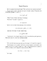
1.4 <strong>The</strong>venin’s <strong>The</strong>orem<br />
Vin<br />
Figure 3: A voltage divider.<br />
<strong>The</strong>venin’s theorem states that any circuit consisting of resistors and EMFs has an equivalent<br />
circuit consisting of a single voltage source VTH in series with a single resistor RTH.<br />
<strong>The</strong> concept of “load” is useful at this point. Consider a partial circuit with two output<br />
points held at potential difference Vout which are not connected to anything. A resistor RL<br />
placed across the output will complete the circuit, allowing current to flow through RL. <strong>The</strong><br />
resistor RL is often said to be the “load” <strong>for</strong> the circuit. A load connected to the output of<br />
our voltage divider circuit is shown in Fig. 4<br />
<strong>The</strong> prescription <strong>for</strong> finding the <strong>The</strong>venin equivalent quantities VTH and RTH is as follows:<br />
• For an “open circuit” (RL →∞), then VTH = Vout .<br />
• For a “short circuit” (RL → 0), then RTH = VTH/Ishort.<br />
An example of this using the voltage divider circuit follows. We wish to find the <strong>The</strong>venin<br />
equivalent circuit <strong>for</strong> the voltage divider.<br />
Vin<br />
R<br />
1<br />
R<br />
1<br />
R<br />
2<br />
Vout<br />
R<br />
2<br />
Vout<br />
R<br />
L<br />
Figure 4: Adding a “load” resistor RL.<br />
3
<strong>The</strong> goal is to deduce VTH and RTH to yield the equivalent circuit shown in Fig. 5.<br />
V TH<br />
R TH<br />
Figure 5: <strong>The</strong> <strong>The</strong>venin equivalent circuit.<br />
To get VTH we are supposed to evaluate Vout when RL is not connected. This is just our<br />
voltage divider result:<br />
� �<br />
R2<br />
VTH = Vin<br />
R1 + R2<br />
Now, the short circuit gives, by Ohm’s Law, Vin = IshortR1. Solving <strong>for</strong> Ishort and combining<br />
with the VTH result gives<br />
RTH = VTH/Ishort = R1R2<br />
R1 + R2<br />
Note that this is the equivalent parallel resistance of R1 and R2.<br />
This concept turns out to be very useful, especially when different circuits are connected<br />
together, and is very closely related to the concepts of input and output impedance (or<br />
resistance), as we shall see.<br />
4<br />
R L
1.5 <strong>The</strong>venin <strong>The</strong>orem (contd.)<br />
Class <strong>Notes</strong> 2<br />
Recall that the <strong>The</strong>venin <strong>The</strong>orem states that any collection of resistors and EMFs is equivalent<br />
to a circuit of the <strong>for</strong>m shown within the box labelled “Circuit A” in the figure below.<br />
As be<strong>for</strong>e, the load resistor RL is not part of the <strong>The</strong>venin circuit. <strong>The</strong> <strong>The</strong>venin idea,<br />
however, is most useful when one considers two circuits or circuit elements, with the first<br />
circuit’s output providing the input <strong>for</strong> the second circuit. In Fig. 6, the output of the<br />
first circuit (A), consisitng of VTH and RTH, is fed to the second circuit element (B), which<br />
consists simply of a load resistance (RL) to ground. This simple configuration represents, in<br />
a general way, a very broad range of analog electronics.<br />
V TH<br />
Circuit A<br />
R TH<br />
1.5.1 Avoiding Circuit Loading<br />
Vout<br />
Figure 6: Two interacting circuits.<br />
Circuit B<br />
VTH is a voltage source. In the limit that RTH → 0 the output voltage delivered to the load<br />
RL remains at constant voltage. For finite RTH, the output voltage is reduced from VTH by<br />
an amount IRTH, whereIis the current of the complete circuit, which depends upon the<br />
value of the load resistance RL: I = VTH/(RTH + RL).<br />
<strong>The</strong>re<strong>for</strong>e, RTH determines to what extent the output of the first circuit behaves as an<br />
ideal voltage source. An approximately ideal behavior turns out to be quite desirable in most<br />
cases, as Vout can be considered constant, independent of what load is connected. Since our<br />
combined equivalent circuit (A + B) <strong>for</strong>ms a simple voltage divider, we can easily see what<br />
the requirement <strong>for</strong> RTH can be found from the following:<br />
�<br />
�<br />
RL<br />
Vout = VTH<br />
RTH + RL<br />
5<br />
=<br />
VTH<br />
1+(RTH/RL)<br />
R L
Thus, we should try to keep the ratio RTH/RL small in order to approximate ideal behavior<br />
and avoid “loading the circuit”. A maximum ratio of 1/10 is often used as a design rule of<br />
thumb.<br />
A good power supply will have a very small RTH, typically much less than an ohm. For<br />
a battery this is referred to as its internal resistance. <strong>The</strong> dimming of one’s car headlights<br />
when the starter is engaged is a measure of the internal resistance of the car battery.<br />
1.5.2 Input and Output Impedance<br />
Our simple example can also be used to illustrate the important concepts of input and output<br />
resistance. (Shortly, we will generalize our discussion and substitute the term “impedance”<br />
<strong>for</strong> resistance. We can get a head start by using the common terms “input impedance” and<br />
“output impedance” at this point.)<br />
• <strong>The</strong> output impedance of circuit A is simply its <strong>The</strong>venin equivalent resistance RTH.<br />
<strong>The</strong> output impedance is sometimes called “source impedance”.<br />
• <strong>The</strong> input impedance of circuit B is its resistance to ground from the circuit input. In<br />
this case it is simply RL.<br />
It is generally possible to reduce two complicated circuits, which are connected to each<br />
other as an input/output pair, to an equivalent circuit like our example. <strong>The</strong> input and<br />
output impedances can then be measured using the simple voltage divider equations.<br />
2 RC Circuits in Time Domain<br />
2.0.3 Capacitors<br />
Capacitors typically consist of two electrodes separated by a non-conducting gap. <strong>The</strong><br />
quantitiy capacitance C is related to the charge on the electrodes (+Q on one and −Q on<br />
the other) and the voltage difference across the capacitor by<br />
C = Q/VC<br />
Capacitance is a purely geometric quantity. For example, <strong>for</strong> two planar parallel electrodes<br />
each of area A and separated by a vacuum gap d, the capacitance is (ignoring fringe fields)<br />
C = ɛ0A/d, whereɛ0 is the permittivity of vacuum. If a dielectric having dielectric constant<br />
κ is placed in the gap, then ɛ0 → κɛ0 ≡ ɛ. <strong>The</strong> SI unit of capacitance is the Farad. Typical<br />
laboratory capacitors range from ∼ 1pF to ∼ 1µF.<br />
For DC voltages, no current passes through a capacitor. It “blocks DC”. When a time<br />
varying potential is applied, we can differentiate our defining expression above to get<br />
I = C dVC<br />
dt<br />
<strong>for</strong> the current passing through the capacitor.<br />
6<br />
(1)
Vin<br />
2.0.4 A Basic RC Circuit<br />
R<br />
Figure 7: RC circuit — integrator.<br />
I<br />
C<br />
Vout<br />
Consider the basic RC circuit in Fig. 7. We will start by assuming that Vin is a DC voltage<br />
source (e.g. a battery) and the time variation is introduced by the closing of a switch at<br />
time t = 0. We wish to solve <strong>for</strong> Vout as a function of time.<br />
Applying Ohm’s Law across R gives Vin − Vout = IR. <strong>The</strong> same current I passes through<br />
the capacitor according to I = C(dV/dt). Substituting and rearranging gives (let V ≡ VC =<br />
Vout):<br />
dV<br />
dt<br />
1 1<br />
+ V =<br />
RC RC Vin<br />
<strong>The</strong> homogeneous solution is V = Ae −t/RC ,whereAis a constant, and a particular solution<br />
is V = Vin. <strong>The</strong> initial condition V (0) = 0 determines A, and we find the solution<br />
V (t) =Vin<br />
�<br />
�<br />
−t/RC<br />
1 − e<br />
This is the usual capacitor “charge up” solution.<br />
Similarly, a capacitor with a voltage Vi across it which is discharged through a resistor<br />
to ground starting at t = 0 (<strong>for</strong> example by closing a switch) can in similar fashion be found<br />
to obey<br />
V (t) =Vie −t/RC<br />
2.0.5 <strong>The</strong> “RC Time”<br />
In both cases above, the rate of charge/discharge is determined by the product RC which<br />
has the dimensions of time. This can be measured in the lab as the time during charge-up or<br />
discharge that the voltage comes to within 1/e of its asymptotic value. So in our charge-up<br />
example, Equation 3, this would correspond to the time required <strong>for</strong> Vout to rise from zero<br />
to 63% of Vin.<br />
2.0.6 RC Integrator<br />
From Equation 2, we see that if Vout ≪ Vin then the solution to our RC circuit becomes<br />
Vout = 1<br />
�<br />
RC<br />
Vin(t)dt (4)<br />
7<br />
(2)<br />
(3)
Note that in this case Vin can be any function of time. Also note from our solution Eqn. 3<br />
that the limit Vout ≪ Vin corresponds roughly to t ≪ RC. Within this approximation, we<br />
see clearly from Eqn. 4 why the circuit above is sometimes called an “integrator”.<br />
2.0.7 RC Differentiator<br />
Let’s rearrange our RC circuit as shown in Fig. 8.<br />
Vin<br />
C<br />
I<br />
Figure 8: RC circuit — differentiator.<br />
R<br />
Vout<br />
Applying Kirchoff’s second Law, we have Vin = VC + VR, where we identify VR = Vout.<br />
By Ohm’s Law, VR = IR,whereI=C(dVC/dt) by Eqn. 1. Putting this together gives<br />
Vout = RC d<br />
dt (Vin − Vout)<br />
In the limit Vin ≫ Vout, we have a differentiator:<br />
Vout = RC dVin<br />
dt<br />
By a similar analysis to that of Section 2.0.6, we would see the limit of validity is the opposite<br />
of the integrator, i.e. t ≫ RC.<br />
8
Class <strong>Notes</strong> 3<br />
3 Circuit Analysis in Frequency Domain<br />
We now need to turn to the analysis of passive circuits (involving EMFs, resistors, capacitors,<br />
and inductors) in frequency domain. Using the technique of the complex impedance,<br />
we will be able to analyze time-dependent circuits algebraically, rather than by solving differential<br />
equations. We will start by reviewing complex algebra and setting some notational<br />
conventions. It will probably not be particularly useful to use the text <strong>for</strong> this discussion,<br />
and it could lead to more confusion. Skimming the text and noting results might be useful.<br />
3.1 Complex Algebra and Notation<br />
Let ˜ V be the complex representation of V .<strong>The</strong>nwecanwrite<br />
˜V=ℜ( ˜ V)+ıℑ( ˜ V)=Ve ıθ = V [cos θ + ı sin θ]<br />
where ı = √ −1. V is the (real) amplitude:<br />
�<br />
V = ˜V ˜ V ∗ = �<br />
ℜ 2 ( ˜ V )+ℑ 2 ( ˜ V) �1/2 where ∗ denotes complex conjugation. <strong>The</strong> operation of determining the amplitude of a<br />
complex quantity is called taking the modulus. <strong>The</strong> phase θ is<br />
θ =tan −1�<br />
ℑ( ˜ V)/ℜ( ˜ V) �<br />
So <strong>for</strong> a numerical example, let a voltage have a real part of 5 volts and an imaginary part<br />
of3volts. <strong>The</strong>n ˜ V =5+3ı= √ 34e ı tan−1 (3/5) .<br />
Note that we write the amplitude of ˜ V , <strong>for</strong>med by taking its modulus, simply as V .Itis<br />
often written | ˜ V |. We will also use this notation if there might be confusion in some context.<br />
Since the amplitude will in general be frequency dependent, it will also be written as V (ω).<br />
We will most often be interested in results expressed as amplitudes, although we will also<br />
look at the phase.<br />
3.2 Ohm’s Law Generalized<br />
Our technique is essentially that of the Fourier trans<strong>for</strong>m, although we will not need to<br />
actually invoke that <strong>for</strong>malism. <strong>The</strong>re<strong>for</strong>e, we will analyze our circuits using a single Fourier<br />
frequency component, ω =2πf. This is perfectly general, of course, as we can add (or<br />
integrate) over frequencies if need be to recover a result in time domain. Let our complex<br />
Fourier components of voltage and current be written as ˜ V = Ve ı(ωt+φ1) and Ĩ = Ie ı(ωt+φ2) .<br />
Now, we wish to generalize Ohm’s Law by replacing V = IR by ˜ V = Ĩ ˜ Z,where ˜ Zis the<br />
(complex) impedance of a circuit element. Let’s see if this can work. We already know that<br />
aresistorRtakes this <strong>for</strong>m. What about capacitors and inductors?<br />
Our expression <strong>for</strong> the current through a capacitor, I = C(dV/dt) becomes<br />
Ĩ = C d<br />
dt Veı(ωt+φ1) = ıωC ˜ V<br />
9
Thus, we have an expression of the <strong>for</strong>m ˜ V = Ĩ ˜ ZC <strong>for</strong> the impedance of a capacitor, ˜ ZC, if<br />
we make the identification ˜ ZC =1/(ıωC).<br />
For an inductor of self-inductance L, the voltage drop across the inductor is given by<br />
Lenz’s Law: V = L(dI/dt). (Note that the voltage drop has the opposite sign of the induced<br />
EMF, which is usually how Lenz’s Law is expressed.) Our complex generalization leads to<br />
˜V = L d d<br />
Ĩ = L<br />
dt dt Ieı(ωt+φ2) = ıωLĨ<br />
So again the <strong>for</strong>m of Ohm’s Law is satisfied if we make the identification ˜ ZL = ıωL.<br />
To summarize our results, Ohm’s Law in the complex <strong>for</strong>m ˜ V = Ĩ ˜ Z canbeusedto<br />
analyze circuits which include resistors, capacitors, and inductors if we use the following:<br />
• resistor of resistance R: ˜ ZR = R<br />
• capacitor of capacitance C: ˜ ZC =1/(ıωC) =−ı/(ωC)<br />
• inductor of self-inductance L: ˜ ZL = ıωL<br />
3.2.1 Combining Impedances<br />
It is significant to point out that because the algebraic <strong>for</strong>m of Ohm’s Law is preserved,<br />
impedances follow the same rules <strong>for</strong> combination in series and parallel as we obtained <strong>for</strong><br />
resistors previously. So, <strong>for</strong> example, two capacitors in parallel would have an equivalent<br />
impedance given by 1/ ˜ Zp =1/ ˜ Z1+1/ ˜ Z2. Using our definition ˜ ZC = −ı/ωC, we then recover<br />
the familiar expression Cp = C1 + C2. So we have <strong>for</strong> any two impedances in series (clearly<br />
generalizing to more than two):<br />
˜Zs = ˜ Z1 + ˜ Z2<br />
And <strong>for</strong> two impedances in parallel:<br />
˜Zp = �<br />
1/ ˜ Z1 +1/ ˜ �−1 Z2 = ˜ Z1 ˜ Z2<br />
˜Z1+ ˜ Z2<br />
And, accordingly, our result <strong>for</strong> a voltage divider generalizes (see Fig. 9) to<br />
˜Vout = ˜ Vin<br />
˜Z1 + ˜ Z2<br />
Now we are ready to apply this technique to some examples.<br />
3.3 A High-Pass RC Filter<br />
�<br />
<strong>The</strong> configuration we wish to analyze is shown in Fig. 10. Note that it is the same as Fig. 7<br />
of the notes. However, this time we apply a voltage which is sinusoidal: ˜ Vin(t) =Vine ı(ωt+φ) .<br />
As an example of another common variation in notation, the figure indicates that the input<br />
is sinusoidal (“AC”) by using the symbol shown <strong>for</strong> the input. Note also that the input and<br />
output voltages are represented in the figure only by their amplitudes Vin and Vout, which<br />
also is common. This is fine, since the method we are using to analyze the circuit (complex<br />
impedances) shouldn’t necessarily enter into how we describe the physical circuit.<br />
10<br />
˜Z2<br />
�<br />
(5)
Vin<br />
~<br />
Vin Z 1<br />
Z 2<br />
~<br />
V out<br />
Figure 9: <strong>The</strong> voltage divider generalized.<br />
C<br />
Figure 10: A high-pass filter.<br />
R<br />
Vout<br />
We see that we have a generalized voltage divider of the <strong>for</strong>m discussed in the previous<br />
section. <strong>The</strong>re<strong>for</strong>e, from Eqn. 5 we can write down the result if we substitute ˜ Z1 = ˜ ZC =<br />
−ı/(ωC) and ˜ Z2= ˜ ZR=R:<br />
˜Vout = ˜ �<br />
�<br />
R<br />
Vin<br />
R − ı/(ωC)<br />
At this point our result is general, and includes both amplitude and phase in<strong>for</strong>mation.<br />
Often, we are only interested in amplitudes. We can divide by ˜ Vin on both sides and find<br />
the amplitude of this ratio (by multiplying by the complex conjugate then taking the square<br />
root). <strong>The</strong> result is often referred to as the transfer function of the circuit, which we can<br />
designate by T (ω).<br />
T (ω) ≡ | ˜ Vout|<br />
| ˜ Vin|<br />
= Vout<br />
Vin<br />
=<br />
ωRC<br />
[1 + (ωRC) 2 ] 1/2<br />
Examine the behavior of this function. Its maximum value is one and minimum is<br />
zero. You should convince yourself that this circuit attenuates low frequencies and “passes”<br />
(transmits with little attenuation) high frequencies, hence the term high-pass filter. <strong>The</strong><br />
cutoff between high and low frequencies is conventionally described as the frequency at<br />
which the transfer function is 1/ √ 2. This is approximately equal to an attenuation of 3<br />
decibels, which is a description often used in engineering (see below). From Eqn. 6 we see<br />
that T =1/ √ 2 occurs at a frequency<br />
(6)<br />
2πf3db = ω3db =1/(RC) (7)<br />
11
<strong>The</strong> decibel scale works as follows: db= 20 log 10(A1/A2), where A1 and A2 represent any<br />
real quantity, but usually are amplitudes. So a ratio of 10 corresponds to 20 db, a ratio of 2<br />
corresponds to 6 db, √ 2 is approximately 3 db, etc.<br />
3.4 A Low-Pass RC Filter<br />
An analogy with the analysis above, we can analyze a low-pass filter, as shown in Fig. 11.<br />
Vin<br />
R<br />
Figure 11: A low-pass filter.<br />
You should find the following result <strong>for</strong> the transfer function:<br />
T (ω) ≡ | ˜ Vout|<br />
| ˜ Vin|<br />
= Vout<br />
Vin<br />
=<br />
1<br />
C<br />
[1 + (ωRC) 2 ] 1/2<br />
Vout<br />
You should verify that this indeed exhibits “low pass” behavior. And that the 3 db<br />
frequency is the same as we found <strong>for</strong> the high-pass filter:<br />
(8)<br />
2πf3db = ω3db =1/(RC) (9)<br />
We note that the two circuits above are equivalent to the circuits we called “differentiator”<br />
and “integrator” in Section 2. However, the concept of high-pass and low-pass filters is much<br />
more general, as it does not rely on an approximation.<br />
An aside. One can compare our results <strong>for</strong> the RC circuit using the complex impedance<br />
technique with what one would obtain by starting with the differential equation (in time) <strong>for</strong><br />
an RC circuit we obtained in Section 2, taking the Fourier trans<strong>for</strong>m of that equation, then<br />
solving (algebraically) <strong>for</strong> the trans<strong>for</strong>m of Vout. It should be the same as our result <strong>for</strong> the<br />
amplitude Vout using impedances. After all, that is what the impedance technique is doing:<br />
trans<strong>for</strong>ming our time-domain <strong>for</strong>muation to one in frequency domain, which, because of<br />
the possibility of analysis using a single Fourier frequency component, is particularly simple.<br />
This is discussed in more detail in the next notes.<br />
12
Class <strong>Notes</strong> 4<br />
3.5 Frequency Domain Analysis (contd.)<br />
Be<strong>for</strong>e we look at some more examples using our technique of complex impedance, let’s look<br />
at some related general concepts.<br />
3.5.1 Reactance<br />
First, just a redefintion of what we already have learned. <strong>The</strong> term reactance is often used<br />
in place of impedance <strong>for</strong> capacitors and inductors. Reviewing our definitions of impedances<br />
from Section 3.2 we define the reactance of a capacitor ˜ XC to just be equal to its impedance:<br />
˜XC ≡−ı/(ωC). Similarly, <strong>for</strong> an inductor ˜ XL ≡ ıωL. This is the notation used in the text.<br />
However, an alternative but common useage is to define the reactances as real quantities.<br />
This is done simply by dropping the ı from the definitions above. <strong>The</strong> various reactances<br />
present in a circuit can by combined to <strong>for</strong>m a single quantity X, which is then equal to the<br />
imaginary part of the impedance. So, <strong>for</strong> example a circuit with R, L, andCin series would<br />
have total impedance<br />
˜Z = R + ıX = R + ı(XL + XC) =R+ı(ωL − 1<br />
ωC )<br />
A circuit which is “reactive” is one <strong>for</strong> which X is non-negligible compared with R.<br />
3.5.2 General Solution<br />
As stated be<strong>for</strong>e, our technique involves solving <strong>for</strong> a single Fourier frequency component<br />
such as ˜ V = Ve ı(ωt+φ) . You may wonder how our results generalize to other frequencies and<br />
to input wave<strong>for</strong>ms other than pure sine waves. <strong>The</strong> answer in words is that we Fourier<br />
decompose the input and then use these decomposition amplitudes to weight the output we<br />
found <strong>for</strong> a single frequency, Vout. We can <strong>for</strong>malize this within the context of the Fourier<br />
trans<strong>for</strong>m, whch will also allow us to see how our time-domain differential equation became<br />
trans<strong>for</strong>med to an algebraic equation in frequency domain.<br />
Consider the example of the RC low-pass filter, or integrator, circuit of Fig. 7. We<br />
obtained the differential equation given by Eq. 2. We wish to take the Fourier trans<strong>for</strong>m of<br />
this equation. Define the Fourier trans<strong>for</strong>m of V (t) as<br />
v(ω)≡F{V(t)}= 1<br />
� +∞<br />
√ dte<br />
2π −∞<br />
−ıωt V (t) (10)<br />
Recall that F{dV/dt} = ıωF{V}. <strong>The</strong>re<strong>for</strong>e our differential equation becomes<br />
Solving <strong>for</strong> v(ω) gives<br />
ıωv(ω)+v(ω)/(RC) =F{Vin(t)}/(RC) (11)<br />
v(ω)= F{Vin(t)}<br />
1+ıωRC<br />
13<br />
(12)
<strong>The</strong> general solution is then the real part of the inverse Fourier trans<strong>for</strong>m:<br />
˜V (t) =F −1 {v(ω)}= 1<br />
� +∞<br />
√ dω<br />
2π −∞<br />
′ e ıω′ t ′<br />
v(ω ) (13)<br />
In the specific case we have considered so far of a single Fourier component of frequency<br />
ω, i.e. ˜ Vin = Vie ıωt ,thenF{ ˜ Vin(t)} = √ 2πδ(ω − ω ′ ), and we recover our previous result <strong>for</strong><br />
the transfer function:<br />
˜T = ˜ V/ ˜ 1<br />
Vin =<br />
(14)<br />
1+ıωRC<br />
For an arbitrary functional <strong>for</strong>m <strong>for</strong> Vin(t), one could use Eqns. 12 and 13. Note that<br />
one would go through the same steps if Vin(t) werewrittenasaFourierseriesratherthan<br />
a Fourier integral. Note also that the procedure carried out to give Eqn. 11 is <strong>for</strong>mally<br />
equivalent to our use of the complex impedances: In both cases the differential equation is<br />
converted to an algebraic equation.<br />
3.6 Phase Shift<br />
We now need to discuss finding the phase φ of our solution. To do this, we proceed as previously,<br />
<strong>for</strong> example like the high-pass filter, but this time we preserve the phase in<strong>for</strong>mation<br />
by not taking the modulus of ˜ Vout. <strong>The</strong> input to a circuit has the <strong>for</strong>m ˜ Vin = Vine ı(ωt+φ1) ,<br />
and the output ˜ Vout = Voute ı(ωt+φ2) . We are usually only interested in the phase difference<br />
φ2 − φ1 between input and output, so, <strong>for</strong> convenience, we can choose φ1 =0andsetthe<br />
phase shift to be φ2 ≡ φ. Physically, we must choose the real or imaginary part of these<br />
expressions. Conventionally, the real part is used. So we have:<br />
Vin(t) =ℜ( ˜ Vin) =Vin(ω)cos(ωt)<br />
and<br />
Vout(t) =ℜ( ˜ Vout) =Vout(ω)cos(ωt + φ)<br />
Let’s return to our example of the high-pass filter to see how to calculate the phase shift.<br />
We rewrite the expression from Section 3.3 and then multiply numerator and denominator<br />
by the complex conjugate of the denominator:<br />
˜Vout = ˜ �<br />
�<br />
R<br />
Vin<br />
R − ı/(ωC)<br />
ıωt 1+ı/(ωRC)<br />
= Vine<br />
1+1/(ωRC) 2<br />
By recalling the general <strong>for</strong>m a + ıb = √ a 2 + b 2 e ıφ ,whereφ=tan −1 (b/a), we can write<br />
1+ı/(ωRC) =<br />
allowing us to read off the phase shift:<br />
Our solution <strong>for</strong> ˜ Vout is then<br />
�<br />
1+<br />
� �2 1<br />
ωRC<br />
�1/2 e ıφ<br />
φ =tan −1 (1/(ωRC)) (15)<br />
Vine<br />
˜Vout =<br />
ıωt+φ<br />
�<br />
1+( 1<br />
ωRC )2<br />
�1/2 14
This, of course, yields the same | ˜ Vout| as we found be<strong>for</strong>e in Eqn. 6 of Section 3.3. But now<br />
we also have included the phase in<strong>for</strong>mation. <strong>The</strong> “real” time-dependent solution is then<br />
just the real part of this:<br />
where φ is given by Eqn. 15.<br />
3.7 Power in Reactive Circuits<br />
Vout(t) =ℜ( ˜ Vout) =Vout cos(ωt + φ)<br />
Recall that <strong>for</strong> DC voltages and currents the power associated with a circuit element carrying<br />
current I with voltage change V is just P = VI. Now, <strong>for</strong> time-varying voltages and currents<br />
we have to be more careful. We could still define an instantaneous power as the product<br />
V (t)I(t). However, it is generally more useful to average the power over time.<br />
3.7.1 General Result <strong>for</strong> AC<br />
Since we are considering Fourier components, we will average the results over one period<br />
T =1/f =2π/ω. <strong>The</strong>re<strong>for</strong>e, the time-averaged power is<br />
� T<br />
= 1<br />
V(t)I(t)dt<br />
T 0<br />
where the brackets indicate the time average. Let the voltage and current be out of phase<br />
by an arbitrary phase angle φ. So we have V(t)=V0cos(ωt) andI(t)=I0cos(ωt + φ).<br />
We can plug these into the expression <strong>for</strong> and simplify using the following: cos(ωt +<br />
φ) =cos(ωt)cos(φ) − sin(ωt)sin(φ); � T<br />
0 sin(ωt)cos(ωt)dt =0;and(1/T ) � T<br />
0 sin2 (ωt)dt =<br />
(1/T ) � T<br />
0 cos2 (ωt)dt =1/2. This yields<br />
= 1<br />
2 V0I0cos φ = VRMSIRMS cos φ (16)<br />
In the latter expression we have used the “root mean squared”, or RMS, amplitudes. Using<br />
voltage as an example, the RMS and standard amplitudes are related by<br />
VRMS ≡<br />
� 1<br />
T<br />
� T<br />
0<br />
V 2 (t)dt<br />
� 1/2<br />
=<br />
� 1<br />
T<br />
3.7.2 Power Using Complex Quantities<br />
� T<br />
0<br />
V 2<br />
0 cos2 �1/2 (ωt)dt<br />
Our results above can be simply expressed in terms of ˜ V and<br />
start with ˜ V (t) =V0e ıωt and Ĩ(t) =I0e ı(ωt+φ) .Bynotingthat<br />
ℜ( ˜ V ∗ Ĩ)=ℜ(V0I0(cos φ + ı sin φ)) = V0I0 cos φ<br />
we identify an expression <strong>for</strong> average power which is equivalent to Eqn. 16 :<br />
= V0/ √ 2 (17)<br />
Ĩ. Equivalent to above, we<br />
= 1<br />
2 ℜ(˜ V ∗ Ĩ)= 1<br />
2 ℜ(˜ V Ĩ∗ ) (18)<br />
15
Vin<br />
L C<br />
Figure 12: A RLC circuit. Several filter types are possible depending upon how Vout is<br />
chosen. In the case shown, the circuit gives a resonant output.<br />
3.8 An RLC Circuit Example<br />
We can apply our technique of impedance to increasingly more intricate examples, with no<br />
more ef<strong>for</strong>t than a commensurate increase in the amount of algebra. <strong>The</strong> RLC circuit of Fig.<br />
12 exemplifies some new qualitative behavior.<br />
We can again calculate the output using our generalized voltage divider result of Eqn. 5.<br />
In this case, the ˜ Z1 consists of the inductor and capacitor in series, and ˜ Z2 is simply R. So,<br />
˜Z1=ıωL − ı/(ωC) = ıL<br />
ω<br />
R<br />
�<br />
ω 2 − ω 2 �<br />
0<br />
wherewehavedefinedtheLC resonant frequency ω0 ≡ 1/ √ LC. We then obtain <strong>for</strong> the<br />
transfer function:<br />
T (ω) ≡ | ˜ Vout|<br />
| ˜ Vin| =<br />
R<br />
|R + ˜ Z1| =<br />
ωγ<br />
[ω 2 γ 2 +(ω 2 −ω 2 0) 2 ] 1/2<br />
where γ ≡ R/L is the “R-L frequency”.<br />
T (ω) indeed exhibits a resonance at ω = ω0. <strong>The</strong> quality factor Q, defined as the ratio<br />
of ω0 to the width of the resonance is given by Q ≈ ω0/(2γ) <strong>for</strong> γ ≪ ω0. Such circuits have<br />
many applications. For example, a high-Q circuit, where Vin(t) is the signal on an antenna,<br />
can be used as a receiver.<br />
As was shown in class, we achieve different behavior if we choose to place the output<br />
across the capacitor or inductor, rather than across the resistor, as above. Rather than a<br />
resonant circuit, choosing Vout = VC yields a low-pass filter of the <strong>for</strong>m<br />
T (ω) = |−ı/(ωC)|<br />
|R + ˜ Z1| =<br />
ω 2 0<br />
[ω 2 γ 2 +(ω 2 −ω 2 0) 2 ] 1/2<br />
<strong>The</strong> cutoff frequency is ω0, and <strong>for</strong> ω ≫ ω0 then T ∼ ω −2 (“12 db per octave”), which more<br />
closely approaches ideal step function-like behavior than the RC low pass filter, <strong>for</strong> which<br />
T ∼ ω −1 <strong>for</strong> ω ≫ ω0 (“6 db per octave”). As you might suspect, choosing Vout = VL provides<br />
a high-pass filter with cutoff at ω0 and T ∼ ω −2 <strong>for</strong> ω ≪ ω0.<br />
16<br />
Vout
3.9 More Filters<br />
3.9.1 Combining Filter Sections<br />
Filter circuits can be combined to produce new filters with modified functionality. An example<br />
is the homework problem (6) of page 59 of the text, where a high-pass and a low-pass<br />
filter are combined to <strong>for</strong>m a “band-pass” filter. As discussed at length in Section 1.5, it<br />
is important to design a “stiff” circuit, in which the next circuit element does not load the<br />
previous one, by requiring that the output impedance of the first be much smaller than the<br />
input impedance of the second. We can standardize this inequality by using a factor of 10<br />
<strong>for</strong> the ratio | ˜ Zin|/| ˜ Zout|.<br />
3.9.2 More Powerful Filters<br />
This technique of cascading filter elements to produce a better filter is discussed in detail in<br />
Chapter 5 of the text. In general, the transfer functions of such filters take the <strong>for</strong>m (<strong>for</strong> the<br />
low-pass case):<br />
T (ω) = �<br />
1+αn(f/fc) 2n�−1/2 where fc is the 3 db frequency, αn is a coefficient depending upon the type of filter, and n is<br />
the filter “order,” often equal to the number of filtering capacitors.<br />
3.9.3 Active Filters<br />
Filters involving LC circuits are very good, better than the simple RC filters, as discussed<br />
above. Un<strong>for</strong>tunately, inductors are, in practice, not ideal lumped circuit elements and are<br />
difficult to fabricate. In addition, filters made entirely from passive elements tend to have<br />
a lot of attenuation. For these reasons active filters are most commonly used where good<br />
filtering is required. <strong>The</strong>se typically use operational amplifiers (which we will discuss later),<br />
which can be configured to behave like inductors, and can have provide arbitrary voltage<br />
gain. Again, this is discussed in some detail in Chapter 5. When we discuss op amps later,<br />
we will look at some examples of very simple active filters. At high frequencies (<strong>for</strong> example<br />
RF), op amps fail, and one most fall back on inductors.<br />
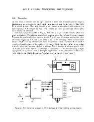
4 Diode Circuits<br />
<strong>The</strong> figure below is from Lab 2, which gives the circuit symbol <strong>for</strong> a diode and a drawing of<br />
a diode from the lab. Diodes are quite common and useful devices. One can think of a diode<br />
as a device which allows current to flow in only one direction. This is an over-simplification,<br />
but a good approximation.<br />
Figure 13: Symbol and drawing <strong>for</strong> diodes.<br />
17<br />
I F
A diode is fabricated from a pn junction. Semi-conductors such as silicon or germanium<br />
can be “doped” with small concentrations of specific impurities to yield a material which<br />
conducts electricity via electron transport (n-type) or via holes (p-type). When these are<br />
brounght together to <strong>for</strong>m a pn junction, electrons (holes) migrate away from the n-type<br />
(p-type) side, as shown in Fig. 14. This redistribution of charge gives rise to a potential gap<br />
∆V across the junction, as depicted in the figure. This gap is ∆V ≈ 0.7 V <strong>for</strong> silicon and<br />
≈ 0.3 V <strong>for</strong> germanium.<br />
V<br />
- - +<br />
p - - + +<br />
- + + n<br />
Figure 14: A pn junction, <strong>for</strong>ming a voltage gap across the junction.<br />
When a diode is now connected to an external voltage, this can effectively increase or<br />
decrease the potential gap. This gives rise to very different behavior, depending upon the<br />
polarity of this external voltage, as shown by the typical V -I plot of Fig. 15. When the<br />
diode is “reverse biased,” as depicted in the figure, the gap increases, and very little current<br />
flows across the junction (until eventually at ∼ 100 V field breakdown occurs). Conversely,<br />
a “<strong>for</strong>ward biased” configuration decreases the gap, approaching zero <strong>for</strong> an external voltage<br />
equal to the gap, and current can flow easily. An analysis of the physics gives the <strong>for</strong>m<br />
I = IS<br />
�<br />
e eV/kT − 1 �<br />
where IS is a constant, V is the applied voltage, and kT/e = 26 mV at room temperature.<br />
Thus, when reverse biased, the diode behaves much like an open switch; and when <strong>for</strong>ward<br />
biased, <strong>for</strong> currents of about 10 mA or greater, the diode gives a nearly constant voltage<br />
drop of ≈ 0.6 V.<br />
18<br />
x<br />
ΔV
-100<br />
V<br />
Reverse Biased<br />
+ -<br />
I<br />
10 mA<br />
1 μΑ<br />
0.7 V<br />
Forward Biased<br />
+ -<br />
Figure 15: <strong>The</strong> V -I behavior of a diode.<br />
19<br />
V
Class <strong>Notes</strong> 5<br />
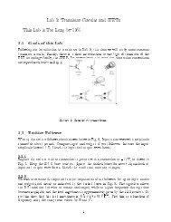
5 Transistors and Transistor Circuits<br />
Although I will not follow the text in detail <strong>for</strong> the discussion of transistors, I will follow<br />
the text’s philosophy. Unless one gets into device fabrication, it is generally not important<br />
to understand the inner workings of transistors. This is difficult, and the descriptions which<br />
one gets by getting into the intrinsic properties are not particularly satisfying. Rather, it is<br />
usually enough to understand the extrinsic properties of transistors, treating them <strong>for</strong> the<br />
most part as a black box, with a little discussion about the subtleties which arise from within<br />
the black box.<br />
In practice, one usually confronts transistors as components of pre-packaged circuits, <strong>for</strong><br />
example in the operational amplifier circuits which we will study later. However, I have<br />
found that it is very useful to understand transistor behavior even if one rarely builds a<br />
transistor circuit in practice. <strong>The</strong> ability to analyze the circuit of an instrument or device is<br />
quite valuable.<br />
We will start, as with Chapter 2 of the text, with bipolar transistors. <strong>The</strong>re are other<br />
common technologies used, particularly FET’s, which we will discuss later. However, most<br />
of what you know can be carried over directly by analogy. Also, we will assume npn type<br />
transistors, except where it is necessary to discuss pnp. For circuit calculations, one simply<br />
reverses all signs of relevant currents and voltages in order to translate npn to pnp.<br />
5.1 Connections and Operating Mode<br />
Below we have the basic connection definitions <strong>for</strong> bipolar transistors as taken from the text.<br />
As indicated in the figure, and as you determined in lab, the base-emitter and base-collector<br />
pairs behave somewhat like diodes. Do not take this too literally. In particular, <strong>for</strong> the basecollector<br />
pair this description is far off the mark. We will refer to the transistor connections<br />
as C, B, andE.<br />
Figure 16: Bipolar transistor connections.<br />
20
5.1.1 Rules <strong>for</strong> Operation<br />
Let’s start by stating what needs to be done to a transistor to make it operate as a transistor.<br />
Suppose we have the following:<br />
1. VC >VE,byatleastafew ×0.1 V.<br />
2. VB >VE<br />
3. VC >VB<br />
4. We do not exceed maximum ratings <strong>for</strong> voltage differences or currents.<br />
When these conditions are not met, then (approximately) no current flows in or out of the<br />
transistor. When these conditions are met, then current can flow into the collector (and out<br />
the emitter) in proportion to the current flowing into the base:<br />
IC = hFEIB = βIB<br />
where hFE = β is the current gain. (We will use the β notation in these notes.) <strong>The</strong> value<br />
of the current gain varies from transistor type to type, and within each type, too. However,<br />
typically β ≈ 100. Unless otherwise specified, we will assume β = 100 when we need a<br />
number. From Figure 17 below and Kirchoff’s first law, we have the following relationship<br />
among the currents:<br />
IE = IB + IC = IB + βIB =(β+1)IB ≈IC<br />
As we will see below, the transistor will “try” to achieve its nominal β. This will not always<br />
be possible, in which case the transistor will still be on, but IC
5.1.2 Transistor Switch and Saturation<br />
From the preceding discussion, the most straight<strong>for</strong>ward way to turn the transistor “on” or<br />
“off” is by controlling VBE. This is illustrated by the circuit below which was introduced in<br />
Lab 2. We will follow the lab steps again here.<br />
R<br />
+5 V<br />
33<br />
LED<br />
2N2222A<br />
Figure 18: A transistor switch.<br />
First, let R = 10 kΩ. When the switch is open, IC = βIB = 0, of course. When the switch<br />
is closed, then VBE becomes positive and VB = VE +0.6=0.6V.IB =(5−0.6)/10 4 =0.44<br />
mA. Hence, IC = βIB = 44 mA. <strong>The</strong>n, assuming negligible voltage drop across the LED,<br />
VC =5−33 × 0.044 = 3.5 V.So,VCE > 0andVCB > 0. So this should work just fine.<br />
Substituting R =1kΩgivesIB =4.4mAandβIB = 440 mA. Setting this equal to<br />
IC would give VC = −9.5 V. This is not possible. In order to stay in operation VCE must<br />
be positive, and depending upon the transistor species, usually can only go as low as ≈ 0.2<br />
V. (Appendix K of the text, pages 1066-1067, gives data <strong>for</strong> a typical model.) Hence, IC is<br />
limited to a maximum value of IC =(5−0.2)/33 ≈ 150 mA. So, effectively, the current gain<br />
has been reduced to β = IC/IB = 150/4.4 = 34. In this mode of operation, the transistor is<br />
said to be saturated. It turns out that <strong>for</strong> high-speed switching applications, <strong>for</strong> example in<br />
computers, the transistors are generally operated in a partially saturated mode, <strong>for</strong> reasons<br />
discussed in Section 2.02 of the text.<br />
5.2 Notation<br />
We will now look at some other typical transistor configurations, including the emitter<br />
follower, the current source, and the common-emitter amplifier. But first we need to set<br />
some notation. We will often be considering voltages or currents which consist of a time<br />
varying signal superposed with a constant DC value. That is,<br />
V (t) =V0+v(t); I(t)=IO+i(t)<br />
where V0 and I0 are the DC quantities, and v or i represent time-varying signals. Hence,<br />
∆V = v ; ∆I = i<br />
22
Typically, we can consider v or i to be sinusoidal functions, e.g. v(t) =vocos(ωt + φ), and<br />
their amplitudes vo and io (sometimes also written as v or i when their is no confusion) are<br />
small compared with V0 or I0, respectively.<br />
5.3 Emitter Follower<br />
<strong>The</strong> basic emitter follower configuration is shown below in Figure 19. An input is fed to<br />
the base. <strong>The</strong> collector is held (by a voltage source) to a constant DC voltage, VCC. <strong>The</strong><br />
emitter connects to a resistor to ground and an output. As we shall see, the most useful<br />
characteristic of this circuit is a large input impedance and a small output impedance.<br />
Vin<br />
Vcc<br />
R<br />
Vout<br />
Figure 19: Basic emitter follower.<br />
For an operating transistor we have Vout = VE = VB − 0.6. Hence, vout = vE = vB. From<br />
this, we can determine the voltage gain G, equivalent to the transfer function, <strong>for</strong> the emitter<br />
follower:<br />
G ≡ vout/vin = vE/vB = 1 (22)<br />
From Eqn. 20, IE =(β+1)IB⇒iE =(β+1)iB. <strong>The</strong>re<strong>for</strong>e, we see that the follower exhibits<br />
“current gain” of output to input equal to β + 1. Assuming the output connection draws<br />
negligible current, we have by Ohm’s Law iE = vE/R. Using this in the previous expression<br />
and solving <strong>for</strong> iB gives iB = iE/(β +1)=(vB/R)/(β + 1). Now we can define the input<br />
impedance of the follower:<br />
Zin = vin/iin = vB/iB = R(β + 1) (23)<br />
By applying the <strong>The</strong>venin definition <strong>for</strong> equivalent impedance, we can also determine the<br />
output impedance of the follower:<br />
Zout = vin/iE = =<br />
(β +1)iB<br />
Zsource<br />
(24)<br />
β +1<br />
where Zsource is the source (i.e. output) impedance of the circuit which gave rise to vin.<br />
Hence, the emitter follower effectively increases input impedance (compared to R) bya<br />
factor β +1≈100 and reduces output impedance, relative to that of the source impedance<br />
of the previous circuit element, by a factor β +1≈100. We will return to this point next<br />
time.<br />
23<br />
vin
Class <strong>Notes</strong> 6<br />
Following our discussion last time of the basic transistor switch and emitter follower, we<br />
will likewise introduce the basic relations <strong>for</strong> two other transistor circuit configurations: the<br />
current source and the common-emitter amplifier. We will then return to the issue of input<br />
and output impedance so that we can build realistic circuits using these configurations.<br />
5.4 Transistor Current Source<br />
Figure 20 illustrates the basic configuration <strong>for</strong> a single-transistor current source. VCC is<br />
a constant positive voltage from a DC power supply. Hence, the base voltage VB is also a<br />
constant, with VB = VCCR2/(R1 + R2). RL represents a load which we intend to power with<br />
a current which is approximately independent of the specific value of RL.<br />
R 1<br />
V B<br />
R 2<br />
V cc<br />
I B<br />
R C<br />
R E<br />
Figure 20: Basic transistor current source.<br />
When the transistor is on, we have IE =(β+1)IB. In addition, we have VE = VB−0.6; and<br />
VE = IERE =(β+1)IBRE. Solving <strong>for</strong> IB in this last equation gives IB = VE/((β +1)RE).<br />
We can combine these to solve <strong>for</strong> the current which passes through RL:<br />
VE<br />
IL = IC = βIB = β =<br />
(β +1)RE<br />
β VB−0.6 ≈<br />
β+1 RE<br />
VB−0.6 (25)<br />
RE<br />
Hence, we see that indeed IL is independent of RL.<br />
Of course, there are limitations to the range of RL <strong>for</strong> which the current source behavior<br />
is reasonable. Recall that the transistor will shut down if VB ≤ VE or if VCE is less than<br />
≈ 0.2 V. <strong>The</strong>se criteria determine the compliance of the current source, that is its useful<br />
operating range. So, <strong>for</strong> example, if we have VCC =15VandVB = 5 V in our circuit above,<br />
then VE =5−0.6=4.4V, and the range of compliance <strong>for</strong> the collector voltage VC will be<br />
approximately 4.6 Vto15V.<br />
24<br />
I C<br />
I E
5.5 Common-emitter Amplifier<br />
Figure 21 represents the basic configuration of the common-emitter amplifier. To determine<br />
the output <strong>for</strong> this circuit, we assume at this point that the input is a sum of a DC offset<br />
voltage V0 and a time-varying signal vin, as discussed last time. (In the next section we will<br />
discuss how to achieve these.) V0 provides the transistor “bias”, so that VB >VE,andthe<br />
signal of interest is vin.<br />
V in<br />
R C<br />
R E<br />
V cc<br />
V out<br />
Figure 21: Basic common-emitter amplifier.<br />
<strong>The</strong> incoming signal shows up on the emitter: vin =∆(VE+0.6)=∆VE≡vE.Andby Ohm’s Law, iE = vE/RE = vB/RE. As we found previously, iE = iC + iB ≈ iC. Now, the<br />
voltage at the output is Vout = VC = VCC − ICRC. And there<strong>for</strong>e, ∆Vout ≡ vout = −iCRC.<br />
Putting all of this together, vout = −iCRC ≈−iERC =−(vB/RE) RC, giving the voltage<br />
gain G:<br />
G ≡ vout/vin = −RC/RE<br />
(26)<br />
5.6 Circuit Biasing and Input<br />
Now we need to figure out how to provide inputs to our basic circuits. In Fig. 22 below we<br />
show the input network <strong>for</strong> a common-emitter amplifier. <strong>The</strong> same considerations we apply<br />
here apply equally to the input of an emitter follower. <strong>The</strong> idea is that the voltage divider<br />
R1 and R2 provide the DC bias voltage (V0 in our discussion above), and the time varying<br />
signal is input through the capacitor (which blocks the DC). We need to figure out what<br />
design criteria should be applied to this design.<br />
We need to make sure that our input circuit does not load the amplifier, C is chosen<br />
to give a reasonable RC cutoff, and that the gain of the amplifier is what we want. We<br />
will start by designing the DC component of the input network, that is choosing R1 and<br />
R2. It is helpful when designing the input network to consider the equivalent circuit shown<br />
in Fig. 23. <strong>The</strong> diode and resistor labelled Zin represent the transistor input: the voltage<br />
drop across the base-emitter “diode” and the input impedance from Eqn. 23. RTH is the<br />
<strong>The</strong>nenin equivalent resistance <strong>for</strong> the DC input network.<br />
So our design procedure can be as follows:<br />
25
V in<br />
C<br />
R 1<br />
R 2<br />
V cc<br />
R C<br />
R E<br />
V out<br />
Figure 22: Common-emitter amplifier with input network.<br />
V TH<br />
R TH<br />
I B<br />
Z in<br />
V B<br />
Figure 23: Equivalent circuit <strong>for</strong> design of DC input network.<br />
1. Choose RTH ≪ Zin = RE(β +1).<br />
2. Determine R1 and R2 based on the equivalent circuit.<br />
3. Choose C to provide a proper high-pass cutoff frequency.<br />
4. Choose the amplifier gain, if need be.<br />
26
Class <strong>Notes</strong> 7<br />
5.7 Transistor Differential Amplifier<br />
Differential amplifiers are in general very useful. <strong>The</strong>y consist of two inputs and one output,<br />
as indicated by the generic symbol in Fig. 24. <strong>The</strong> output is proportional to the difference<br />
between the two inputs, where the proportionality constant is the gain. One can think of<br />
this as one of the two inputs (labelled “−”) being inverted and then added to the other<br />
non-inverting input (labelled “+”). Operational amplifiers (“op amps”), which we will soon<br />
study, are fancy differential amplifiers, and are represented by the same symbol as that of<br />
Fig. 24.<br />
in 1<br />
in 2<br />
+<br />
-<br />
Figure 24: Symbol <strong>for</strong> a differential amplifier or op amp.<br />
This technique is commonly used to mitigate noise pickup. For example, a signal which<br />
is to be transmitted and subject to noise pickup can first be replicated and inverted. This<br />
“differential pair” is then transmitted and then received by a differential amplifier. Any<br />
noise pickup will be approximately equal <strong>for</strong> the two inputs, and hence will not appear in<br />
the output of the differential amplifer. This “common mode” noise is rejected. This is often<br />
quantified by the common-mode rejection ratio (CMRR) which is the ratio of differential<br />
gain to common-mode gain. Clearly, a large CMRR is good.<br />
5.7.1 A Simple Design<br />
<strong>The</strong> circuit shown in Fig. 25 represents a differential amplifier design. It looks like two<br />
common-emitter amplifiers whose emitters are tied together at point A. In fact, the circuit<br />
does behave in this way. It is simplest to analyze its output if one writes each input as the<br />
sum of two terms, a sum and a difference. Consider two signals v1 and v2. In general, we<br />
can rewrite these as v1 = +∆v/2 andv2 = −∆v/2, where =(v1+v2)/2is<br />
the average and ∆v = v1 − v2 is the difference. <strong>The</strong>re<strong>for</strong>e, we can break down the response<br />
of the circuit to be due to the response to a common-mode input () and a difference<br />
(∆v) input.<br />
Let’s analyze the difference signal first. <strong>The</strong>re<strong>for</strong>e, consider two inputs v1 =∆v/2 and<br />
v2=−∆v/2. <strong>The</strong> signals at the emitters then follow the inputs, as usual, so that at point A<br />
we have vA = vE1 + vE2 = v1 + v2 = 0. Following the common-emitter amplifier derivation,<br />
we have vout1 = −iCRC, whereiC ≈iE =vE/RE = vin1/RE. Hence, vout1 = −(RC/RE)v1<br />
and vout2 = −(RC/RE)v2. We define the differential gain Gdiff as the ratio of the output to<br />
the input difference. So<br />
Gdiff1 ≡ vout1/∆v = −(RC/RE)v1/(2v1) =−RC/(2RE)<br />
27<br />
out
In 1<br />
and similarly <strong>for</strong> output 2<br />
R C<br />
Out 1<br />
R E<br />
A<br />
VCC<br />
RE<br />
REE<br />
V<br />
EE<br />
R C<br />
Out 2<br />
In 2<br />
Figure 25: Differential amplifier design.<br />
Gdiff2 ≡ vout2/∆v = −(RC/RE)v2/(−2v2) =RC/(2RE)<br />
Generally, only one of the two ouputs is used. Referring back to Fig. 24, we see that if we<br />
were to choose our one output to be the one labelled “out2”, then “in1” would correspond to<br />
“+” (non-inverting input) and “in2” would correspond to “−” (inverting input). Keeping in<br />
mind these results <strong>for</strong> the relative signs, it is usual to write the differential gain as a positive<br />
quantity:<br />
Gdiff = RC<br />
2RE<br />
where the sign depends upon which is used.<br />
Now consider the common mode part of the inputs: v1<br />
following relations:<br />
iEE = iE1 + iE2 =2iE;<br />
= v2 =< v>. We have the<br />
VA =VEE + IEEREE ⇒ vA = iEEREE =2iEREE ;<br />
iE = vE − vA<br />
Solving <strong>for</strong> iE in the last equation gives:<br />
RE<br />
�<br />
iE = vin<br />
= vin − 2iEREE<br />
RE<br />
1<br />
RE +2REE<br />
Again following the derivation <strong>for</strong> the the common-emitter amplifie, we have vout = −iCRC ≈<br />
−iERC. So each output has the same common-mode gain:<br />
Gcom ≡ vout<br />
vin<br />
RC<br />
�<br />
= −<br />
RE +2REE<br />
28<br />
(27)<br />
(28)
<strong>The</strong> ratio of the differential to common-mode gain (ignoring the sign) then gives the<br />
CMRR:<br />
CMRR = RE +2REE<br />
2RE<br />
≈ REE<br />
RE<br />
where <strong>for</strong> a typical design REE ≫ RE.<br />
Building on what we learned, we can easily improve our differential amplifier design by<br />
adding an emitter-follower stage to the output and a replacing the resistor REE with a<br />
current source. This is discussed briefly in the next two sections.<br />
5.7.2 Adding a Follower<br />
<strong>The</strong> output impedance of the common-emitter configuration, as used in the differential amplifer,<br />
Zout ≈ RC, is not always as small as one would like. This can be easily improved<br />
by adding an emitter follower to the output. Hence, the input of the follower would be<br />
connected to the output of the differential amplifier. As discussed be<strong>for</strong>e, the follower then<br />
produces an output impedance which is ≈ β + 1 times smaller than the preceding stage.<br />
Hence, in this case, we would have Zout ≈ RC/β. <strong>The</strong> follower’s emitter resistor (call it<br />
R ′ E), of course, has to be consistent with our impedance non-loading criteria, in this case<br />
βR ′ E ≫ RC.<br />
5.7.3 Adding a Current Source<br />
In our expression <strong>for</strong> CMRR above, we see that a large REE improves per<strong>for</strong>mance. However,<br />
this can also significantly load the voltage source of VEE, producing non-ideal behavior.<br />
Hence, REE is limited in practice. A solution to this which is commonly used is to replace<br />
REE by the output of a current source. In other words, point “A” in Fig. 25 would be<br />
connected to the collector of a current source such as that of Fig. 20. This can be justified<br />
by noting that the dynamic impedance provided by REE is given by vA/iEE. By limiting<br />
variations in iEE, as provided by a current source, one effectively achieves a large dynamic<br />
impedance.<br />
To implement this one has to decide what quiescent current is required <strong>for</strong> the current<br />
source and what the quiescent voltage of the collector should be. <strong>The</strong> latter is given by the<br />
quiescent voltage at the inputs of the differential amplifier. For example, if the inputs are<br />
DC ground, then point “A” will be at approximately −0.6 V, depending upon any voltage<br />
drop across RE.<br />
5.7.4 No Emitter Resistor<br />
One variation of the above is to remove the emitter resistor. In this case one replaces RE in<br />
the expressions above with the intrinsic emitter resistance discussed in Section 5.8.1 below:<br />
RE → re = 25mV/IC<br />
To be exact, one should replace RE in our equations with the series resistance of RE and re:<br />
RE → RE + re. However, in most practical situations RE ≫ re.<br />
29<br />
(29)
Class <strong>Notes</strong> 8<br />
5.8 More on Transistor Circuits<br />
5.8.1 Intrinsic Emitter Resistance<br />
One consequence of the Ebers-Moll equation, which we will discuss later, is that the transistor<br />
emitter has an effective resistance which is given by<br />
re = 25mV/IC<br />
This is illustrated in Fig. 26. Essentially one can treat this as any other resistance. So<br />
in most of our examples so far in which an emitter resistor RE is present, one can simply<br />
replace RE by the series sum RE + re. Numerically, typical values reveal that re is safely<br />
ignored. For example, IC =1mAgivesre =25Ω,whereasRE might be typically ∼ 1 kΩ.<br />
<strong>The</strong> exception is an emitter follower output, where the output voltage is divided by re and<br />
RE. In some cases an external emitter resistor RE is omitted, in which case RE → re in our<br />
previous expressions.<br />
b<br />
c<br />
e<br />
re b e<br />
Figure 26: Intrinsic emitter resistance.<br />
5.8.2 Input and Output Impedance of the Common-Emitter Amplifer<br />
For convenience, the basic common-emitter amplifier is reproduced below. <strong>The</strong> calculation of<br />
the input impedance does not differ from that we used <strong>for</strong> the emitter follower in Section 5.3.<br />
That is, the input impedance is Zin = RE(β + 1). <strong>The</strong> output impedance is quite different<br />
from that of the emitter follower, however. Consider our definition of output impedance in<br />
terms of the <strong>The</strong>venin equivalent circuit:<br />
Zout =<br />
vout<br />
i(RL → 0)<br />
<strong>The</strong> numerator is just the usual vout we calculated in Eqn. 26. Hence, vout = vin(RC/RE).<br />
<strong>The</strong> short current is just iC, and since iC =(β/(β +1))iE≈iE =vin/RE, thenwehaveour<br />
result<br />
Zin =(β+1)RE ; Zout ≈ RC (30)<br />
Note that these results apply equally well to the differential amplifier configuration, which<br />
is, as we said be<strong>for</strong>e, essentially two coupled common-emitter amplifiers.<br />
30
V in<br />
5.8.3 DC Connections and Signals<br />
R C<br />
R E<br />
V cc<br />
V out<br />
Figure 27: Basic common-emitter amplifier.<br />
We already discussed in class the fact that <strong>for</strong> a configuration like that of the input network<br />
of Fig. 22, that the input time-varying signal vin is not affected by the DC offsets of the<br />
resistor connections. In other words, R1 and R2 appear, <strong>for</strong> a time-varying signal, to be both<br />
connected to ground. Hence, when designing the cutoff frequency <strong>for</strong> the input high-pass<br />
filter, the effective resistance is just the usual parallel resistance of R1, R2, and the transistor<br />
input impedance RE(β +1).<br />
5.9 Ebers-Moll Equation and Transistor Realism<br />
With the exception of saturation effects and a mention of the intrinsic emitter resistance<br />
re, we have so far considered transistors in a reather idealized manner. To understand<br />
many of the most important aspects of transistor circuits, this approach is reasonable. For<br />
example, we have treated the current gain β of a non-saturated transistor to be independent<br />
of currents, temperature, etc. In reality, this is not the case. One of the finer points of<br />
circuit design is to take care to eliminate a strong dependence of the circuit behavior on<br />
such complications. We start with the Ebers-Moll equation, which gives a foundation <strong>for</strong><br />
understanding one class of complications.<br />
5.9.1 Ebers-Moll Equation<br />
Our simple relationship <strong>for</strong> collector current <strong>for</strong> an operating transistor, IC = βIB is an<br />
idealization. We can see from the plots of Appendix K (cf pg. 1076-7) that β indeed does<br />
depend on various parameters. A more precise description is via the Ebers-Moll equation:<br />
IC = IS<br />
�<br />
e VBE/VT − 1 �<br />
≈ ISe VBE/VT (31)<br />
where VT ≡ kT/e = (25.3 mV)(T/298 K), IS = IS(T ) is the saturation current, and<br />
VBE ≡ VB − VE, as usual. Since typically VBE ≈ 600mV ≫ VT , then the exponential term<br />
is much larger than 1, and IS ≪ IC. Since IBis also a function of VBE, thenweseethat<br />
β=IC/IB can be thought of as a good approximation <strong>for</strong> a rather complicated situation,<br />
and in fact β is itself a function of IC (or VBE, as well as of temperature.<br />
31
We see that IC is not intrinsically a function of IB, but rather is controlled by VBE. For<br />
this reason, and others, it is often stated that transistor gain is really a transconductance<br />
gain. This means that it takes a voltage input and converts it to a current output. So we<br />
write, in general,<br />
gm = iout/vin<br />
as the transconductance gain. We then recover voltage gain by multiplying gm by the resistor<br />
at the output which converts the output current to a voltage. For example, <strong>for</strong> the commonemitter<br />
amplifier we have iout = −vin/RE and<br />
G = gmRC = −RC/RE<br />
as be<strong>for</strong>e.<br />
<strong>The</strong> base-emitter “diode” implies a relationship between IB and VBE of the <strong>for</strong>m VBE =<br />
V0 ln(IB/I0), where V0 ≈ 0.6 VandI0is a constant. If this <strong>for</strong>m <strong>for</strong> VBE is plugged into Eqn.<br />
31, we recover our previous relationship IC = βIB, where the current gain β is a combination<br />
of the various factors which are slowly-varying functions of temperature and currents.<br />
Another consequence of Ebers-Moll equation is that we see where the intrinsic emitter<br />
resistance re, which we introduced last time, comes from. By definition,<br />
1/re = iE/vBE ≈ iC/vBE = dIC<br />
From Eqn. 31, the derivative is simply IC/VT .Sowehave<br />
where VT is again as above.<br />
5.9.2 <strong>The</strong> Current Mirror<br />
re=VT/IC<br />
dVBE<br />
Figure 28 shows a very commonly used current source circuit known as the current mirror.<br />
Understanding its principle of operation requires the Ebers-Moll equation. <strong>The</strong> “programming<br />
current” IP defines the collector current of the left-hand transistor. (<strong>The</strong> base<br />
currents should be negligibly small.) From the Ebers-Moll equation, this collector current<br />
then uniquely determines VBE. <strong>The</strong> collector-base connection transfers this well-defined base<br />
voltage to the collector, thus maintaining the voltage drop across the programming resistor.<br />
<strong>The</strong> right-hand transistor is “matched” to the left-hand one. That is, the pair were manufactured<br />
together to have nearly identical properties. So this right-hand transistor assumes<br />
a nearly identical collector current to that which is programmed. Thus the load current<br />
becomes IL = IP . Besides transferring the program current to a load at another point of<br />
the circuit, the current mirror also has the advantage of having a larger range of compliance<br />
than the standard single-transistor current source we studied earlier.<br />
5.9.3 Other Non-ideal Effects<br />
<strong>The</strong> following represent some of the important departures from ideal transistor behavior:<br />
• VBE = VBE(T ). As discussed above, the base-emitter “diode” includes a Boltzmann<br />
factor temperature dependence. This can be linearized, as given in the text, to yield<br />
approximately<br />
∆VBE<br />
∆T ≈−2.1×10⁻³ V/ ◦ C<br />
32<br />
.<br />
(32)
I P<br />
R P<br />
• Early Effect. VBE depends on VCE:<br />
V cc<br />
I L<br />
R L<br />
Figure 28: Current mirror.<br />
∆VBE<br />
∆VCE<br />
≈−1×10 −4<br />
• Miller effect. This affects high-frequency response. <strong>The</strong> reverse-biased “diode” between<br />
base and collector produces a capacitive coupling. Just as emitter resistance<br />
is effectively multiplied by β + 1 <strong>for</strong> input signals, so too this CCB, which is ususally<br />
a few pF, appears to input signals as a capacitance (1 + G)CCB to ground, where G<br />
is the voltage gain of the transistor configuration. Hence, when combined with input<br />
source resistance, this is effectively a low-pass RC filter, and the amplifier response <strong>for</strong><br />
frequencies above the RC cutoff will be greatly reduced. <strong>The</strong> usual solution <strong>for</strong> mitigating<br />
the Miller effect is to reduce the source impedance. This can be effectively done<br />
by coupling to a second transistor with small source resistance at base. <strong>The</strong> cascode<br />
configuration, discussed in the text, uses this. Another example is the single-input<br />
DC differential amplifier, <strong>for</strong> which there is no collector resistor at the input transistor<br />
(this eliminates ∆VC even though the source resistance may be non-negligible), and<br />
the output transistor has grounded base (there<strong>for</strong>e with very small source resistance),<br />
• Variation in gain. <strong>The</strong> β may be quite different from transistor to transistor, even of<br />
the same model. <strong>The</strong>re<strong>for</strong>e circuit designs should not rely on a specific gain, other<br />
than to assume that β ≫ 1.<br />
To illustrate this last point, consider our earlier one transistor current source. We determined<br />
that the load current can be written<br />
� ��VB �<br />
β −VBE<br />
IL =<br />
(33)<br />
β +1<br />
RE + re<br />
where the intrinsic emitter resistance re has been included. <strong>The</strong>re<strong>for</strong>e, the variation in IL<br />
induced by variation in β is<br />
∆IL<br />
IL<br />
= 1<br />
IL<br />
dIL<br />
dβ<br />
∆β =<br />
33<br />
�<br />
1<br />
�<br />
∆β<br />
β +1 β
Hence, variations in β are attenuated by the factor β + 1. So this represents a good design.<br />
<strong>The</strong> variation in the output of this current source resulting from the Early effect can be<br />
evaluated similarly:<br />
∆IL<br />
IL<br />
= 1<br />
IL<br />
dIL<br />
dVBE<br />
∆VBE = − ∆VBE<br />
VB − VBE<br />
= 1 × 10⁻⁴<br />
∆VCE<br />
VB − VBE<br />
which can be evaluated using the compliance range <strong>for</strong> ∆VCE.<br />
Temperature dependence can now be estimated, as well. Using our current source, again,<br />
to exemplify this point, we see that temperature dependence can show up both in VBE and<br />
β. <strong>The</strong> <strong>for</strong>mer effect can be evaluated using the chain rule and the result from the previous<br />
paragraph:<br />
dIL<br />
dT<br />
= dIL<br />
dVBE<br />
dVBE<br />
dT ≈ 2.1 mV/◦ C<br />
RE<br />
<strong>The</strong>re<strong>for</strong>e, we see that temperature dependence is ∝ 1/RE. As be<strong>for</strong>e, RE is in general<br />
replaced by the sum RE + re. In the case where the external resistor is omitted, then the<br />
typically small re values can induce a large temperature dependence (cf problem 7 at the<br />
end of Chapter 2 of the text). Similarly, using previous results, we can estimate the effect<br />
of allowing β = β(T ):<br />
dIL<br />
dT<br />
= dIL<br />
dβ<br />
dβ<br />
dT<br />
= IL<br />
β +1<br />
� �<br />
1dβ<br />
βdT<br />
where the term in parentheses, the fractional gain temperature dependence, is often a known<br />
parameter (cf problem 2d at the end of Chapter 2 of the text).<br />
34
6 Op-Amp Basics<br />
Class <strong>Notes</strong> 9<br />
<strong>The</strong> operational amplifier is one of the most useful and important components of analog electronics.<br />
<strong>The</strong>y are widely used in popular electronics. <strong>The</strong>ir primary limitation is that they<br />
are not especially fast: <strong>The</strong> typical per<strong>for</strong>mance degrades rapidly <strong>for</strong> frequencies greater than<br />
about 1 MHz, although some models are designed specifically to handle higher frequencies.<br />
<strong>The</strong> primary use of op-amps in amplifier and related circuits is closely connected to the<br />
concept of negative feedback. Feedback represents a vast and interesting topic in itself. We<br />
will discuss it in rudimentary terms a bit later. However, it is possible to get a feeling <strong>for</strong> the<br />
two primary types of amplifier circuits, inverting and non-inverting, by simply postulating<br />
a few simple rules (the “golden rules”). We will start in this way, and then go back to<br />
understand their origin in terms of feedback.<br />
6.1 <strong>The</strong> Golden Rules<br />
<strong>The</strong> op-amp is in essence a differential amplifer of the type we discussed in Section 5.7 with<br />
the refinements we discussed (current source load, follower output stage), plus more, all<br />
nicely debugged, characterized, and packaged <strong>for</strong> use. Examples are the 741 and 411 models<br />
which we use in lab. <strong>The</strong>se two differ most significantly in that the 411 uses JFET transistors<br />
at the inputs in order to achieve a very large input impedance (Zin ∼ 10 9 Ω), whereas the<br />
741 is an all-bipolar design (Zin ∼ 10 6 Ω).<br />
<strong>The</strong> other important fact about op-amps is that their open-loop gain ishuge. Thisisthe<br />
gain that would be measured from a configuration like Fig. 29, in which there is no feedback<br />
loop from output back to input. A typical open-loop voltage gain is ∼ 10 4 –10 5 . By using<br />
negative feedback, we throw most of that away! We will soon discuss why, however, this<br />
might actually be a smart thing to do.<br />
in 1<br />
in 2<br />
+<br />
-<br />
out<br />
Figure 29: Operational amplifier.<br />
<strong>The</strong> golden rules are idealizations of op-amp behavior, but are nevertheless very useful<br />
<strong>for</strong> describing overall per<strong>for</strong>mance. <strong>The</strong>y are applicable whenever op-amps are configured<br />
with negative feedback, as in the two amplifier circuits discussed below. <strong>The</strong>se rules consist<br />
of the following two statements:<br />
1. <strong>The</strong> voltage difference between the inputs, V+ − V−, is zero.<br />
(Negative feedback will ensure that this is the case.)<br />
35
2. <strong>The</strong> inputs draw no current.<br />
( This is true in the approximation that the Zin of the op-amp is much larger than any<br />
other current path available to the inputs.)<br />
When we assume ideal op-amp behavior, it means that we consider the golden rules to be<br />
exact. We now use these rules to analyze the two most common op-amp configurations.<br />
6.2 Inverting Amplifier<br />
<strong>The</strong> inverting amplifier configuration is shown in Fig. 30. It is “inverting” because our<br />
signal input comes to the “−” input, and there<strong>for</strong>e has the opposite sign to the output. <strong>The</strong><br />
negative feedback is provided by the resistor R2 connecting output to input.<br />
R1 VIN -<br />
+<br />
VOUT R 2<br />
Figure 30: Inverting amplifier configuration.<br />
We can use our rules to analyze this circuit. Since input + is connected to ground, then<br />
by rule 1, input − is also at ground. For this reason, the input − is said to be at virtual<br />
ground. <strong>The</strong>re<strong>for</strong>e, the voltage drop across R1 is vin − v− = vin, and the voltage drop across<br />
R2 is vout − v− = vout. So, applying Kirchoff’s first law to the node at input −, wehave,<br />
using golden rule 2:<br />
i− =0=iin + iout = vin/R1 + vout/R2<br />
or<br />
G = vout/vin = −R2/R1<br />
(34)<br />
<strong>The</strong> input impedance, as always, is the impedance to ground <strong>for</strong> an input signal. Since<br />
the − input is at (virtual) ground, then the input impedance is simply R1:<br />
Zin = R1<br />
<strong>The</strong> output impedance is very small (< 1 Ω), and we will discuss this again soon.<br />
6.3 Non-inverting Amplifier<br />
This configuration is given in Fig. 31. Again, its basic properties are easy to analyze in<br />
terms of the golden rules.<br />
� �<br />
R1<br />
vin = v+ = v− = vout<br />
R1 + R2<br />
36<br />
(35)
where the last expression is from our voltage divider result. <strong>The</strong>re<strong>for</strong>e, rearranging gives<br />
G = vout/vin = R1 + R2<br />
R1<br />
=1+ R2<br />
<strong>The</strong> input impedance in this case is given by the intrinsic op-amp input impedance. As<br />
mentioned above, this is very large, and is typically in the following range:<br />
V IN<br />
R1<br />
(36)<br />
Zin ∼ 10 8 to 10 12 Ω (37)<br />
R 1<br />
6.4 Departures from Ideal<br />
+<br />
-<br />
R 2<br />
V OUT<br />
Figure 31: Non-inverting amplifier configuration.<br />
It is no surprise that the golden rules are not exact. On the other hand, they generally<br />
describe most, if not all, observed op-amp behavior. Here are some departures from ideal<br />
per<strong>for</strong>mance.<br />
• Offset voltage, VOS. Recall that the input of the op-amp is a differential pair. If the<br />
two transistors are not perfectly matched, an offset will show up as a non-zero DC<br />
offset at the output. As you found in Lab 4, this can be zeroed externally. This offset<br />
adjustment amounts to changing the ratio of currents coming from the emitters of the<br />
two input transistors.<br />
• Bias current, Ibias. <strong>The</strong> transistor inputs actually do draw some current, regardless<br />
of golden rule 2. Those which use bipolar input transistors (e.g. the 741) draw more<br />
current than those which use FETs (e.g. the 411). <strong>The</strong> bias current is defined to be<br />
the average of the currents of the two inputs.<br />
• Offset current, IOS. This is the difference between the input bias currents. Each bias<br />
current, after passing through an input resitive network, will effectively offer a voltage<br />
to the op-amp input. <strong>The</strong>re<strong>for</strong>e, an offset of the two currents will show up as a voltage<br />
offset at the output.<br />
37
Perhaps the best way to beat these efects, if they are a problem <strong>for</strong> a particular application,<br />
is to choose op-amps which have good specifications. For example, IOS can be a<br />
problem <strong>for</strong> bi-polar designs, in which case choosing a design with FET inputs will usually<br />
solve the problem. However, if one has to deal with this, it is good to know what to do. Figure<br />
32 shows how this might be accomplished. Without the 10 kΩ resistors, this represents<br />
a non-inverting amplifier with voltage gain of 1 + (10 5 /10 2 ) ≈ 1000. <strong>The</strong> modified design in<br />
the figure gives a DC path from ground to the op-amp inputs which are aproximately equal<br />
in resistance (10 kΩ), while maintaining the same gain.<br />
IN<br />
10k<br />
Figure 32: Non-inverting amplifier designed to minimize effect of IOS.<br />
Similarly, the inverting amplifier configuration can be modified to mitigate offset currents.<br />
In this case one would put a resistance from the − input to ground which is balanced by the<br />
R1 and R2 in parallel (see Fig. 30).<br />
It is important to note that, just as we found <strong>for</strong> transistor circuits, one shpould always<br />
provide a DC path to ground <strong>for</strong> op-amp inputs. Otherwise, charge will build up on the<br />
effective capacitance of the inputs and the large gain will convert this voltage (= Q/C) into<br />
a large and uncontrolled output voltage offset.<br />
However, our modified designs to fight IOS have made our op-amp designs worse in a<br />
general sense. For the non-inverting design, we have turned the very large input impedance<br />
into a not very spectacular 10 kΩ. In the inverting case, we have made the virtual ground<br />
into an approximation. One way around this, if one is concerned only with AC signals, is<br />
to place a capacitor in the feedback loop. For the non-inverting amplifier, this would go in<br />
series with the resistor R1 to ground. <strong>The</strong>re<strong>for</strong>e, as stated be<strong>for</strong>e, it is best, where important,<br />
to simply choose better op-amps!<br />
6.5 Frequency-dependent Feedback<br />
Below are examples of simple integrator and differentiator circuits which result from making<br />
the feedback path have frequency dependence, in these cases single-capacitor RC filters. It is<br />
also possible to modify non-inverting configurations in a similar way. For example, problem<br />
(3) on page 251 of the text asks about adding a “rolloff” capacitor in this way. Again, one<br />
would simply modify our derivations of the basic inverting and non-inverting gain <strong>for</strong>mulae<br />
by the replacements R → Z, as necessary.<br />
38<br />
10k<br />
100<br />
+<br />
-<br />
100k<br />
OUT
6.5.1 Integrator<br />
Using the golden rules <strong>for</strong> the circuit of Fig. 33, we have<br />
vin − v−<br />
=<br />
R<br />
vin<br />
R = iin = iout = −C d(vout − v−)<br />
= −C<br />
dt<br />
dvout<br />
dt<br />
So, solving <strong>for</strong> the output gives<br />
vout = − 1<br />
�<br />
vindt (38)<br />
RC<br />
And <strong>for</strong> a single Fourier component ω, this gives <strong>for</strong> the gain<br />
G(ω) =− 1<br />
(39)<br />
ωRC<br />
<strong>The</strong>re<strong>for</strong>e, to the extent that the golden rules hold, this circuit represents an ideal integrator<br />
and a low-pass filter. Because of the presence of the op-amp, this is an example of an<br />
active filter. In practice, one may need to supply a resistor in parallel with the capacitor to<br />
give a DC path <strong>for</strong> the feedback.<br />
6.5.2 Differentiator<br />
IN<br />
R<br />
-<br />
+<br />
C<br />
OUT<br />
Figure 33: Op-amp integrator or low-pass filter.<br />
<strong>The</strong> circuit of Fig. 34 can be analyzed in analogy to the integrator. We find the following:<br />
vout = −RC dvin<br />
(40)<br />
dt<br />
G(ω) =−ωRC (41)<br />
So this ideally represents a perfect differentiator and an active high-pass filter. In practice,<br />
one may need to provide a capacitor in parallel with the feedback resistor. (<strong>The</strong> gain cannot<br />
really increase with frequency indefinitely!)<br />
6.6 Negative Feedback<br />
As we mentioned above, the first of our Golden Rules <strong>for</strong> op-amps required the use of<br />
negative feedback. We illustrated this with the two basic negative feedback configurations:<br />
the inverting and the non-inverting configurations. In this section we will discuss negative<br />
feedback in a very general way, followed by some examples illustrating how negative feedback<br />
can be used to improve per<strong>for</strong>mance.<br />
39
6.6.1 Gain<br />
IN<br />
C<br />
-<br />
+<br />
R<br />
OUT<br />
Figure 34: Op-amp differentiator or high-pass filter.<br />
Consider the rather abstract schematic of a negative feedback amplifier system shown in Fig.<br />
35. <strong>The</strong> symbol ⊗ is meant to indicate that negative feedback is being added to the input.<br />
<strong>The</strong> op-amp device itself has intrinsic gain A. This is called the op-amp’s open-loop gain since<br />
this is the gain the op-amp would have in the absence of the feedback loop. <strong>The</strong> quantity B is<br />
the fraction of the output which is fed back to the input. For example, <strong>for</strong> the non-inverting<br />
amplifier this is simply given by the feedback voltage divider: B = R1/(R1 + R2). <strong>The</strong> gain<br />
of the device is, as usual, G = vout/vin. G is often called the closed-loop gain. Tocomplete<br />
the terminology, the product AB is called the loop gain.<br />
vin +<br />
a<br />
A<br />
vout<br />
-<br />
Figure 35: General negative feedback configuration.<br />
As a result of the negative feedback, the voltage at the point labelled “a” in the figure is<br />
B<br />
va = vin − Bvout<br />
<strong>The</strong> amplifier then applies its open-loop gain to this voltage to produce vout:<br />
Now we can solve <strong>for</strong> the closed-loop gain:<br />
vout = Ava = Avin − ABvout<br />
A<br />
vout/vin ≡ G =<br />
(42)<br />
1+AB<br />
Note that there is nothing in our derivation which precludes having B (or A) be a function<br />
of frequency.<br />
40
6.6.2 Input and Output Impedance<br />
We can now also calculate the effect that the closed-loop configuration has on the input<br />
and output impedance. <strong>The</strong> figure below is meant to clearly show the relationship between<br />
the definitions of input and output impedances and the other quantities of the circuit. <strong>The</strong><br />
quantity Ri represents the open-loop input impedance of the op-amp, that is, the impedance<br />
the hardware had in the absence of any negative feedback loop. Similarly, Ro represents the<br />
<strong>The</strong>venin source (output) impedance of the open-loop device.<br />
v<br />
in<br />
b<br />
R i<br />
B<br />
Figure 36: Schematic to illustrate the input and output impedance of a negative feedback<br />
configuration.<br />
We start the calculation of Zin with the definition Zin = vin/iin. Let us calculate the<br />
current passing through Ri:<br />
iin = vin − vb<br />
Substituting the result of Eqn. 42 gives<br />
iin = 1<br />
�<br />
Rearanging allows one to obtain<br />
Ri<br />
Ri<br />
vin − Bvin<br />
R o<br />
= vin − Bvout<br />
Ri<br />
�<br />
A<br />
1+AB<br />
��<br />
v out<br />
Zin = vin/iin = Ri [1 + AB] (43)<br />
A similar procedure allows the calculation of Zout ≡ vopen/ishort. We have vopen = vout<br />
and the shorted current is what gets when the load has zero input impedance. This means<br />
that all of the current from the amplifier goes into the load, leaving none <strong>for</strong> the feedback<br />
loop. Hence, B =0and<br />
ishort = A (vin − Bvout) /Ro = Avin/Ro = Avout<br />
RoG =<br />
This gives our result<br />
� Avout<br />
Ro<br />
Zout = vopen/ishort = Ro<br />
1+AB<br />
41<br />
�� �<br />
1+AB<br />
A<br />
= vout<br />
Ro<br />
(1 + AB)<br />
(44)
<strong>The</strong>re<strong>for</strong>e, the efect of the closed loop circuit is to improve both input and output<br />
impedances by the identical loop-gain factor 1 + AB ≈ AB. So <strong>for</strong> a typical op-amp like a<br />
741 with A =10 3 ,Ri =1MΩ,andRo = 100 Ω, then if we have a loop with B =0.1weget<br />
Zin = 100 MΩ and Zout =1Ω.<br />
6.6.3 Examples of Negative Feedback Benefits<br />
We just demonstrated that the input and output impedance of a device employing negative<br />
feedback are both improved by a factor 1 + AB ≈ AB, the device loop gain. Now we give a<br />
simple example of the gain equation Eqn. 42 in action.<br />
An op-amp may typically have an open-loop gain A which varies by at least an order<br />
of magnitude over a useful range of frequency. Let Amax =10 4 and Amin =10 3 ,andlet<br />
B=0.1. We then calculate <strong>for</strong> the corresponding closed-loop gain extremes:<br />
Gmax = 104<br />
1+10 3 ≈10(1 − 10−3 )<br />
Gmin = 103<br />
1+10 2 ≈10(1 − 10−2 )<br />
Hence, the factor of 10 open-loop gain variation has been reduced to a 1% variation. This<br />
is typical of negative feedback. It attenuates errors which appear within the feedback loop,<br />
either internal or external to the op-amp proper.<br />
In general, the benefits of negative feedback go as the loop gain factor AB. For most<br />
op-amps, A is very large, starting at > 10 5 <strong>for</strong> f
compound circuit instabilities and can lead to oscillating circuits (as we do on purpose <strong>for</strong><br />
the RC relaxation oscillator).<br />
So it is perhaps easy to simply not include such phase shifts in the feedback loop. However,<br />
at high frequencies (f ∼ 1 MHz or more), unintended stray capacitances can become<br />
significant. In fact, within the op-amp circuits themselves, this is almost impossible to<br />
eliminate. Most manufacturers of op-amps confront this issue by intentionally reducing the<br />
open-loop gain at high frequency. This is called compensation. It is carried out by bypassing<br />
one of the internal amplifier stages with a high-pass filter. <strong>The</strong> effect of this is illustrated<br />
in Fig. 37. It is a so-called “Bode plot”, log 10(A) vs log 10(f), showing how the intrinsic<br />
gain of a compensated op-amp (like the 741 or 411) decreases with frequency much sooner<br />
than one without compensation. <strong>The</strong> goal is to achieve A
7 Comparator Circuits<br />
7.1 Simple Comparator<br />
Class <strong>Notes</strong> 10<br />
A comparator can be thought of as a fast, high-gain op-amp which is not used with negative<br />
feedback. This basic idea is shown in Fig. 38. <strong>The</strong> comparator has large open-loop gain A.<br />
<strong>The</strong> function of a comparator is to decide which of the two inputs has larger voltage. We<br />
have in the limit of very large A<br />
�<br />
vout = A(v+ − v−) =<br />
+Vmax v+ >v−<br />
−|Vmin| v+
is low it will, after passing through an inverter, turn the transistor on. In this case, current<br />
sill pass through R and to the emitter connection. This current produces a voltage drop<br />
across R which pulls the output voltage (very close) to the emitter voltage (ground in our<br />
example). Typically R ≈ 1 kΩ. When the comparator inputs are in the complementary<br />
inequality, the transistor is switched off and the output voltage goes to the voltage held by<br />
R, which is +5 V in our example. Using outputs of 0 and +5 V are typical, since these<br />
voltages correspond (roughly) to the TTL convention of digital electronics.<br />
7.2 Schmitt Trigger<br />
A typical circuit using a comparator is shown in Fig. 39. <strong>The</strong> output goes to one of its<br />
two possible states depending upon whether the input v− is greater than or less than the<br />
“threshold” determined by v+. Positive feedback is used to help rein<strong>for</strong>ce the chosen output<br />
state. In this configuration, called the Schmitt trigger, two thresholds can be set, depending<br />
upon which state the output is in. <strong>The</strong> way this works is illustrated in Fig. 40. Vh and<br />
Vl refer to threshold voltages which are set up at the comparator + input by the resistor<br />
divider chain. As long as R3 ≫ R4, the output states will still be determined by the pull-up<br />
resistor R4. For the circuit in the figure, these states are 0 and +5 V. <strong>The</strong> resistor divider,<br />
then sets V+ at different values, depending upon which state the ouput is in. Whether the<br />
connection to +V1 and R1 is required or not depends upon whether a positive threshold is<br />
required when Vout =0.<br />
v in<br />
R 1<br />
R 2<br />
+V 1<br />
-<br />
+<br />
R 3<br />
+5<br />
R 4<br />
Figure 39: Schmitt trigger.<br />
Referring to Fig. 40, we start with Vin = V−
V h<br />
Vl<br />
+5<br />
v in<br />
V out<br />
Figure 40: Examples of Schmitt trigger signals versus time. Top: vin; the dashed lines<br />
indicate the two thresholds set up at the + input of the comparator. Bottom: vout.<br />
Note that the resistor R1 is not necessary if Vl = 0. Also, a negative threshold could be<br />
set in two ways. <strong>The</strong> resistor chain <strong>for</strong>ming the threshold could be connected to negative<br />
voltage, rather than ground, or the emitter of the output transistor could be connected to<br />
negative voltage, thus producing an output with low state at this negative voltage.<br />
7.3 RC Relaxation Oscillator<br />
<strong>The</strong> circuit of Fig. 41 uses both positive and negative feedback. It is called an RC relaxation<br />
oscillator. Note that the positive feedback is a Schmitt configuration. So we expect to have<br />
two thresholds. <strong>The</strong> output voltages are set up to be either +5 V (pull up) or −5 V (emitter<br />
connection). Analysis of the voltage divider reveals that the corresponding two threshold<br />
at V+ will be ±1 V. When the output is +5 V, the capacitor C is charged up through the<br />
resistor R. <strong>The</strong>RC part of the circuit is shown in Fig. 42. As we found in class, the voltage<br />
across the capacitor, and hence the − input to the comparator, is given (after applying initial<br />
conditions) by<br />
Vc(t) =V0− 3V0<br />
2 e(t1−t)/RC<br />
where t1 is the time at which the comparator output is first at V0 = +5 V. Hence, the charge<br />
up curve will eventually cross the +1 V threshold, <strong>for</strong>cing the comparator to the −5 Vstate,<br />
and thereby starting a ramp-down of the capacitor voltage given by<br />
Vc(t) =−V0+ 3V0<br />
2 e(t2−t)/RC<br />
where t2 is the time at which the output switched to −5 V.Thisrampdownwillcrossthe<br />
−1 V threshold, and the whole process will there<strong>for</strong>e repeat indefinitely. <strong>The</strong> output will<br />
be a square wave, whereas Vc resembles a triangle wave. This is a common technique <strong>for</strong><br />
building an oscillator.<br />
46<br />
t<br />
t
100K<br />
10nF<br />
20K<br />
-<br />
+<br />
80K<br />
-5<br />
+5<br />
1K<br />
v out<br />
Figure 41: RC relaxation oscillator.<br />
100K<br />
Vin 10nF<br />
Vout<br />
Figure 42: RC circuit with Vin from the comparator output and Vout going to the − comparator<br />
input of previous figure.<br />
47
8 Radio Basics<br />
Class <strong>Notes</strong> 11<br />
In this section we will discuss some basic concepts concerning signal modulation, generation,<br />
receiving, and demodulation. Some of these concepts are quite general and see applications<br />
in many areas. However, the most familiar perhaps is that of broadcast radio generation<br />
and receiving, hence the title of the section.<br />
We will begin with a simplified discussion of amplitude modulation (AM). From this, we<br />
can see how to carry over many of the concepts to other <strong>for</strong>ms of signal modulation and<br />
reception of signals.<br />
8.1 <strong>The</strong> Case <strong>for</strong> Modulation<br />
Consider the familiar example of radio signals which carry audio in<strong>for</strong>mation. <strong>The</strong> audio<br />
itself has a typical frequency range of<br />
20Hz
f c<br />
+<br />
+<br />
f m<br />
V s<br />
Figure 43: Schematic of modulation.<br />
we can do a “poor man’s” Fourier trans<strong>for</strong>m of Vs:<br />
Vs(t) =Acos ωct + 1<br />
2 Am [cos ((ωc + ωm)t)+cos((ωc−ωm)t)] (46)<br />
So we have a central carrier frequency plus two side-bands at fc ± fm.<br />
One simple way to achieve an amplitude modulated signal is to use an amplifier <strong>for</strong> which<br />
the input is the carrier signal and the amplifier power itself is modulated by the signal, e.g.<br />
VCC − VEE = V0 + V1 cos ωmt, whereV0is the DC offset amd we identify m ∝ V1/V0.<br />
8.3 Detection of AM<br />
8.3.1 Heterodyne Detection<br />
We first consider the simple, but subtle, radio receiver shown in Fig. 44. A real receiver<br />
might include at the input an antenna followed by an LC bandpass filter, with tunable<br />
capacitor. <strong>The</strong> filter is a resonant circuit with a sharp peak at the carrier frequency of the<br />
broadcast ωc =1/ √ LC. <strong>The</strong> Q of the filter is set so that the width of the peak of the<br />
transfer function matches the bandwidth ∆ω of the modulating signal, roughly from ωc −ωm<br />
to ωc + ωm. With this addition, and without the amplified output, the passive “crystal”<br />
radio receiver looks like this.<br />
a R<br />
IN G<br />
OUT<br />
Δω<br />
r<br />
Figure 44: Simple AM receiver.<br />
<strong>The</strong> resistor R and capacitor clearly <strong>for</strong>m a low-pass filter. <strong>The</strong> cutoff frequency would<br />
be set between ωm and ωc in order to keep the in<strong>for</strong>mation encoded by the low-frequency<br />
modulations, and remove the carrier. However, without the diode, the effect would be to<br />
throw away all of the in<strong>for</strong>mation, too, since as we saw from Eqn. 46, all of the frequencies<br />
49<br />
C
of interest are actually in a narrow band centered about the carrier frequency. Without the<br />
diode, the system is linear, and no signal will be present at the output.<br />
<strong>The</strong> diode is non-linear; recall its V -I curve. In order to illustrate how this works, we<br />
assume a specific <strong>for</strong>m <strong>for</strong> the response of a <strong>for</strong>ward-biased diode as I = bV 2 ,wherebis a<br />
constant. A resistor r is inserted between point a and ground (Fig. 44) in order to convert<br />
this diode current to a voltage to be presented to the low-pass filter. Now let V be the linear<br />
combination of two signals: V = V1 cos ω1t + V2 cos ω2t. This then gives rise to an output<br />
current<br />
I = bV 2<br />
1 cos 2 ω1t + bV 2<br />
2 cos 2 ω2t +2bV1V2 cos ω1t cos ω2t<br />
Again using trigonometric identities to <strong>for</strong>m the poor man’s Fourier trans<strong>for</strong>m, this becomes<br />
2I/b = V 2<br />
1<br />
+ V 2<br />
2<br />
+ V 2<br />
1 cos 2ω1t + V 2<br />
2 cos 2ω2t +2V1V2[cos((ω1 + ω2)t)+cos((ω1−ω2)t)]<br />
<strong>The</strong>re<strong>for</strong>e, from the original two frequencies, the diode has produced harmonics (twice the<br />
original), as well as the sum and difference.<br />
In the case of our simplified AM broadcast signal of Eqn. 46, where three frequencies<br />
are originally present (ωc and ωc ± ωm), the effect of the diode is easily generalized from the<br />
steps above using the substitutions ω1 = ωc and ω2 = ωc + ωm or ω2 = ωc − ωm. We find<br />
that the output of the diode will include DC, the first harmonics of all three frequecies, as<br />
well as the six possible sum and difference frequencies. Of particular interest <strong>for</strong> our receiver<br />
is the difference frequency between the carrier and the modulated carrier. For example,<br />
ωc − (ωc − ωm) =ωm<br />
<strong>The</strong>re<strong>for</strong>e, we do in fact recover a Fourier component corresponding to our original modulating<br />
signal. This can then be separated from the higher frequencies using the low-pass filter<br />
and amplifier. This represents a simple example of so-called heterodyne detection, inwhich<br />
different frequencies are combined in order to extract a difference frequency.<br />
As an aside, we note that with our example I = bV 2 , we have squared the input. When<br />
we examine this in frequency domain (Fourier trans<strong>for</strong>m) and low-pass filter the result (averaging),<br />
we have effectively <strong>for</strong>med the so-called power spectrum of the input, also called<br />
the spectral power density.<br />
8.3.2 Harmonic Distortion<br />
Note that we intentionally introduced a non-linear element (the diode) to our system. An unintentional<br />
non-linearity in a circuit, <strong>for</strong> example in an audio amplifier circuit, can introduce<br />
additional frequencies as demonstrated above. In particular, our diode with the I = bV 2 behavior<br />
introduced first harmonics of the original frequencies at twice the original. In general,<br />
a non-linearity may include any number of higher-order terms: I = b1V + b2V 2 + b3V 3 + ···,<br />
where each additional power can generate the next higher harmonic. For example, a nonzero<br />
b3 will generate a 2nd harmonic of the original ω at 3ω. <strong>The</strong> introduction of harmonics<br />
of the input signal is called harmonic distortion. Since the pattern of harmonics is what<br />
distinguishes musical instrument types to the ear, the introduction of non-linearities should<br />
be avoided in high-fidelity audio amplifiers.<br />
8.3.3 Homodyne Detection<br />
An example of this technique is given in the text, pages 653 and 889. It uses a phase-locked<br />
loop (PLL) circuit at the input of the receiver. Recall that the PLL circuit is designed<br />
50
to produce an output which is proportional to shifts in phase of the input. Since one can<br />
consider the modulation of the carrier to be a phase shift (by amount ωmt), the output<br />
of the PLL can then produce a voltage signal proportional to these phase shifts, which in<br />
turn is used to provide active rectification of the input at the frequency of the modulation.<br />
<strong>The</strong> essential non-linear behavior of the diode discussed above is provided in this case by an<br />
active voltage multiplier. This type of PLL circuit is actually more relevant to FM detection,<br />
which is discussed below.<br />
8.3.4 Superheterodyne Detection<br />
This technique is illustrated in the text, pages 895-6. It is essentially a fancy version of our<br />
simple heterodyne detector above. In this case, the simple passive LC bandpass filter at the<br />
input is replaced by a local oscillator and mixer. An example is given in Figure 13.41 of<br />
the text. Consider an input carrier of frequency 10 MHz which has amplitude modulated at<br />
some much lower frequency. This signal is mixed with a local oscillator of fixed frequency<br />
greater than the carrier. In the example of the text, the local oscillator has frequency tuned<br />
to be fLO =10.455 MHz, exactly 455 kHz greater than the carrier. As with our earlier diode<br />
example, the mixed signal includes the difference frequency, in this case 455 kHz, which in<br />
turn has nearby sideband frequencies which differ from 455 kHz by the audio modulation<br />
frequencies. From this point on, the detection is carried out as in the simple heterodyne<br />
example. One advantage here is that a relatively high-frequency carrier, which in general<br />
will be difficult to condition using conventional electronics is effectively reduced to a more<br />
manageable frequency, in the example from 10 MHz to 455 kHz. <strong>The</strong> other advantage is<br />
that the band-pass tuning which follows the mixer is always centered at a constant 455 kHz.<br />
So the tuning is accomplished by adjusting the oscillator, rather than the filter.<br />
8.4 Other Modulation Schemes<br />
Recall from Eqn. 45 that <strong>for</strong> AM the amplitude is modulated by varying the frequency ωm.<br />
However, to preserve the in<strong>for</strong>mation, the generation and receipt of the amplitude must be<br />
linear. In addition, most noise sources will naturally appear as voltages, and hence will add<br />
to the AM signal. On the other hand, phase and frequency modulation (FM) do not suffer<br />
from these complications. Hence, where fidelity is important, these schemes have intrinsic<br />
advantages. Radio broadcast by FM also has the additional advantage, by dint of historical<br />
accident, of occupying a higher frequency band, thus allowing easy accomodation of a full<br />
audio bandwidth. However, unlike the AM radio band, the FM band signals do not reflect<br />
from the ionosphere, and there<strong>for</strong>e can not be transmitted over very large distances (at<br />
night).<br />
8.4.1 Phase Modulation<br />
A carrier of frequency ωc is phase modulated if the resulting signal has the <strong>for</strong>m<br />
V (t) =V0cos(ωct + Ap cos ωmt) (47)<br />
where V0 and Ap are constants and ωm is the modulating frequency, as be<strong>for</strong>e. This can be<br />
expanded, and <strong>for</strong> Ap ≪ 1 can also be simplified:<br />
V (t)/V0 = cosωct cos(Ap cos ωmt) − sin ωct sin(Ap cos ωmt)<br />
51
≈ cos ωct − Ap sin ωct cos ωmt<br />
= cosωct− 1<br />
2 Ap[sin((ωc + ωm)t)+sin((ωc−ωm)t)] (48)<br />
As <strong>for</strong> AM, two new sidebands have appeared, but now they are 90◦ out of phase with<br />
respect to the carrier.<br />
8.4.2 Frequency Modulation<br />
<strong>The</strong> phase of a sinusoidal function, when frequency is a function of time, can in general be<br />
expressed as<br />
�<br />
φ = ωdt<br />
Now suppose the frequency is modulated by a frequency ω about some central carrier frequency<br />
ω = ωc + Af cos ωmt<br />
where Af is a constant. <strong>The</strong>n the phase becomes<br />
φ = ωct + Af<br />
ωm<br />
sin ωmt<br />
Here, Af is called the frequency deviation and Af/ωm is the modulation index <strong>for</strong> FM.<br />
Carrying out steps analogous to those <strong>for</strong> Eqn. 48 gives the following expression <strong>for</strong> the FM<br />
signal:<br />
V (t)/V0 =cosφ=cosωct+ Af<br />
[cos((ωc + ωm)t) − cos((ωc − ωm)t)] (49)<br />
2ωm<br />
So again the Fourier spectrum is similar to what we found <strong>for</strong> AM, except now one of the<br />
two sidebands has amplitude of opposite sign.<br />
8.5 FM Detection<br />
In the AM detection schemes discussed above, the diode or other non-linear element is used<br />
to extract an output signal proportional to cos ωmt, and hence provide a reproduction of the<br />
original modulation, <strong>for</strong> example in the <strong>for</strong>m of an audio signal. For FM detection we need<br />
to replace the diode with something which can provide a voltage output proportional to the<br />
input frequency modulated signal. We explored such a technique in Lab 5 in the <strong>for</strong>m of the<br />
phase-locked loop circuit. <strong>The</strong> PLL scheme is reproduced in Fig. 45. (For this application,<br />
the counter is omitted.) Recall that the signal be<strong>for</strong>e the VCO, labelled Vout, is proportional<br />
to input phase shifts. This is exactly what we need to detect the phase shift introduced by<br />
FM. All that is left is to feed Vout to a low-pass filter and amplifier, as be<strong>for</strong>e.<br />
An apparent practical limitation of this technique <strong>for</strong> FM radio reception is that PLLs do<br />
not operate at these high frequencies (∼ 100 MHz). This is overcome by using the technique<br />
discussed above at the front-end of the superheterodyne receiver. <strong>The</strong> input is mixed using a<br />
local oscillator and the resulting lower frequency (455 kHz in our example) modulated signal<br />
is then input to the PLL. Another technique, called quadrature detection is briefly discusses<br />
in the text, page 652.<br />
52
f<br />
in Phase<br />
Low-pass<br />
Detector<br />
Filter<br />
f<br />
replica<br />
Counter<br />
(divide by n)<br />
f<br />
out<br />
VCO<br />
(V->f)<br />
V out<br />
Figure 45: PLL schematic. Vout provides the FM signal.<br />
53