Lecture Notes for Analog Electronics - The Electronic Universe ...

Class Notes 4
3.5 Frequency Domain Analysis (contd.)
Before we look at some more examples using our technique of complex impedance, let’s look
at some related general concepts.
3.5.1 Reactance
First, just a redefintion of what we already have learned. The term reactance is often used
in place of impedance for capacitors and inductors. Reviewing our definitions of impedances
from Section 3.2 we define the reactance of a capacitor ˜ XC to just be equal to its impedance:
˜XC ≡−ı/(ωC). Similarly, for an inductor ˜ XL ≡ ıωL. This is the notation used in the text.
However, an alternative but common useage is to define the reactances as real quantities.
This is done simply by dropping the ı from the definitions above. The various reactances
present in a circuit can by combined to form a single quantity X, which is then equal to the
imaginary part of the impedance. So, for example a circuit with R, L, andCin series would
have total impedance
˜Z = R + ıX = R + ı(XL + XC) =R+ı(ωL − 1
ωC )
A circuit which is “reactive” is one for which X is non-negligible compared with R.
3.5.2 General Solution
As stated before, our technique involves solving for a single Fourier frequency component
such as ˜ V = Ve ı(ωt+φ) . You may wonder how our results generalize to other frequencies and
to input waveforms other than pure sine waves. The answer in words is that we Fourier
decompose the input and then use these decomposition amplitudes to weight the output we
found for a single frequency, Vout. We can formalize this within the context of the Fourier
transform, whch will also allow us to see how our time-domain differential equation became
transformed to an algebraic equation in frequency domain.
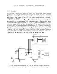
Consider the example of the RC low-pass filter, or integrator, circuit of Fig. 7. We
obtained the differential equation given by Eq. 2. We wish to take the Fourier transform of
this equation. Define the Fourier transform of V (t) as
v(ω)≡F{V(t)}= 1
� +∞
√ dte
2π −∞
−ıωt V (t) (10)
Recall that F{dV/dt} = ıωF{V}. Therefore our differential equation becomes
Solving for v(ω) gives
ıωv(ω)+v(ω)/(RC) =F{Vin(t)}/(RC) (11)
v(ω)= F{Vin(t)}
1+ıωRC
13
(12)