Lecture Notes for Analog Electronics - The Electronic Universe ...

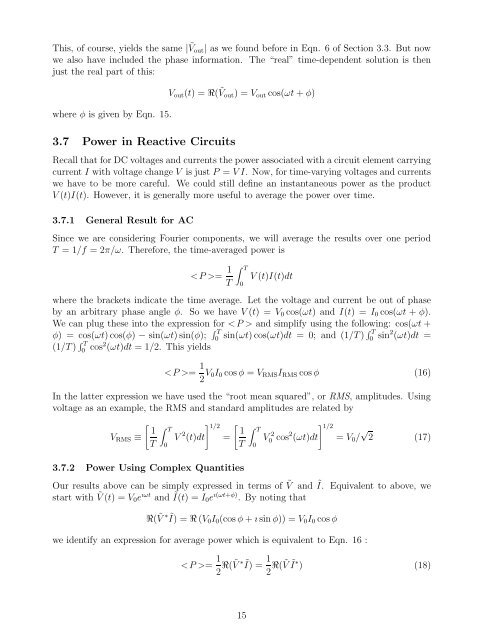
This, of course, yields the same | ˜ Vout| as we found before in Eqn. 6 of Section 3.3. But now
we also have included the phase information. The “real” time-dependent solution is then
just the real part of this:
where φ is given by Eqn. 15.
3.7 Power in Reactive Circuits
Vout(t) =ℜ( ˜ Vout) =Vout cos(ωt + φ)
Recall that for DC voltages and currents the power associated with a circuit element carrying
current I with voltage change V is just P = VI. Now, for time-varying voltages and currents
we have to be more careful. We could still define an instantaneous power as the product
V (t)I(t). However, it is generally more useful to average the power over time.
3.7.1 General Result for AC
Since we are considering Fourier components, we will average the results over one period
T =1/f =2π/ω. Therefore, the time-averaged power is
� T
= 1
V(t)I(t)dt
T 0
where the brackets indicate the time average. Let the voltage and current be out of phase
by an arbitrary phase angle φ. So we have V(t)=V0cos(ωt) andI(t)=I0cos(ωt + φ).
We can plug these into the expression for and simplify using the following: cos(ωt +
φ) =cos(ωt)cos(φ) − sin(ωt)sin(φ); � T
0 sin(ωt)cos(ωt)dt =0;and(1/T ) � T
0 sin2 (ωt)dt =
(1/T ) � T
0 cos2 (ωt)dt =1/2. This yields
= 1
2 V0I0cos φ = VRMSIRMS cos φ (16)
In the latter expression we have used the “root mean squared”, or RMS, amplitudes. Using
voltage as an example, the RMS and standard amplitudes are related by
VRMS ≡
� 1
T
� T
0
V 2 (t)dt
� 1/2
=
� 1
T
3.7.2 Power Using Complex Quantities
� T
0
V 2
0 cos2 �1/2 (ωt)dt
Our results above can be simply expressed in terms of ˜ V and
start with ˜ V (t) =V0e ıωt and Ĩ(t) =I0e ı(ωt+φ) .Bynotingthat
ℜ( ˜ V ∗ Ĩ)=ℜ(V0I0(cos φ + ı sin φ)) = V0I0 cos φ
we identify an expression for average power which is equivalent to Eqn. 16 :
= V0/ √ 2 (17)
Ĩ. Equivalent to above, we
= 1
2 ℜ(˜ V ∗ Ĩ)= 1
2 ℜ(˜ V Ĩ∗ ) (18)
15