Introduction to the resistivity surveying method. The resistivity of ...
Introduction to the resistivity surveying method. The resistivity of ...
Introduction to the resistivity surveying method. The resistivity of ...

Create successful ePaper yourself
Turn your PDF publications into a flip-book with our unique Google optimized e-Paper software.
21<br />
significantly better results. However, it does illustrate <strong>the</strong> advantages <strong>of</strong> using suitable<br />
inversion constrains.<br />
Most field data sets probably lie between <strong>the</strong> two extremes <strong>of</strong> a smoothly varying<br />
<strong>resistivity</strong> and discrete geological bodies with sharp boundaries. If you have a sufficiently fast<br />
computer (Pentium II upwards), and a relatively small data set (2000 datum points or less), it<br />
might be a good idea <strong>to</strong> invert <strong>the</strong> data twice. Once with <strong>the</strong> standard smoothness-constrain<br />
and again with <strong>the</strong> robust model constrain. This will give two extremes in <strong>the</strong> range <strong>of</strong><br />
possible models that can be obtained for <strong>the</strong> same data set. Features that are common <strong>to</strong> both<br />
models are more likely <strong>to</strong> be real.<br />
Some geological bodies have a predominantly horizontal orientation (for example<br />
sedimentary layers and sills) while o<strong>the</strong>rs might have a vertical orientation (such as dykes and<br />
faults). This information can be incorporated in<strong>to</strong> <strong>the</strong> inversion process by setting <strong>the</strong> relative<br />
weights given <strong>to</strong> <strong>the</strong> horizontal and vertical flatness filters. If for example <strong>the</strong> structure has a<br />
predominantly vertical orientation, such as a dyke (Figure 17), <strong>the</strong> vertical flatness filter is<br />
given a greater weight than <strong>the</strong> horizontal filter.<br />
Figure 13. Example <strong>of</strong> inversion results using <strong>the</strong> smoothness-constrain and robust inversion<br />
model constrains. (a) Apparent <strong>resistivity</strong> pseudosection (Wenner array) for a syn<strong>the</strong>tic test<br />
model with a faulted block (100 ohm.m) in <strong>the</strong> bot<strong>to</strong>m-left side and a small rectangular block<br />
(2 ohm.m) on <strong>the</strong> right side with a surrounding medium <strong>of</strong> 10 ohm.m. <strong>The</strong> inversion models<br />
produced by (b) <strong>the</strong> conventional least-squares smoothness-constrained <strong>method</strong> and (c) <strong>the</strong><br />
robust inversion <strong>method</strong>.<br />
Ano<strong>the</strong>r important fac<strong>to</strong>r is <strong>the</strong> quality <strong>of</strong> <strong>the</strong> field data. Good quality data usually<br />
show a smooth variation <strong>of</strong> apparent <strong>resistivity</strong> values in <strong>the</strong> pseudosection. To get a good<br />
model, <strong>the</strong> data must be <strong>of</strong> equally good quality. If <strong>the</strong> data is <strong>of</strong> poorer quality, with<br />
Copyright (1999-2001) M.H.Loke