Introduction to the resistivity surveying method. The resistivity of ...
Introduction to the resistivity surveying method. The resistivity of ...
Introduction to the resistivity surveying method. The resistivity of ...
You also want an ePaper? Increase the reach of your titles
YUMPU automatically turns print PDFs into web optimized ePapers that Google loves.
56<br />
Appendix B<br />
Topographic modelling<br />
In surveys over areas with significant changes in <strong>the</strong> elevation <strong>of</strong> <strong>the</strong> ground surface,<br />
<strong>the</strong> effect <strong>of</strong> <strong>the</strong> <strong>to</strong>pography must be taken in<strong>to</strong> account when carrying out an inversion <strong>of</strong> <strong>the</strong><br />
data set. It is now generally recognised that <strong>the</strong> traditional <strong>method</strong> <strong>of</strong> using <strong>the</strong> “correction<br />
fac<strong>to</strong>rs” for a homogeneous earth model (Fox et al. 1980) does not give sufficiently accurate<br />
results if <strong>the</strong>re are large <strong>resistivity</strong> variations near <strong>the</strong> surface (Tong and Yang 1990). Instead<br />
<strong>of</strong> trying <strong>to</strong> “correct” for <strong>the</strong> effect <strong>of</strong> <strong>the</strong> <strong>to</strong>pography on <strong>the</strong> measurements, <strong>the</strong> preferred<br />
<strong>method</strong> now is <strong>to</strong> incorporate <strong>the</strong> <strong>to</strong>pography in<strong>to</strong> <strong>the</strong> inversion model. <strong>The</strong> RES2DINV<br />
program has 4 different <strong>method</strong>s that can be used <strong>to</strong> incorporate <strong>the</strong> <strong>to</strong>pography in<strong>to</strong> <strong>the</strong><br />
inversion model. One <strong>method</strong> that uses <strong>the</strong> finite-difference <strong>method</strong>, and three based on <strong>the</strong><br />
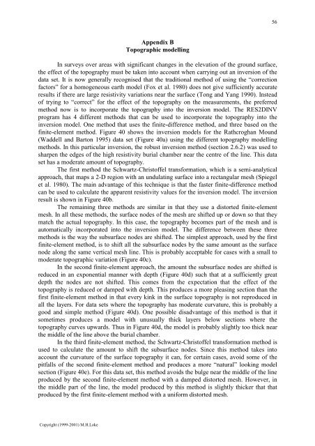
finite-element <strong>method</strong>. Figure 40 shows <strong>the</strong> inversion models for <strong>the</strong> Rathcroghan Mound<br />
(Waddell and Bar<strong>to</strong>n 1995) data set (Figure 40a) using <strong>the</strong> different <strong>to</strong>pography modelling<br />
<strong>method</strong>s. In this particular inversion, <strong>the</strong> robust inversion <strong>method</strong> (section 2.6.2) was used <strong>to</strong><br />
sharpen <strong>the</strong> edges <strong>of</strong> <strong>the</strong> high <strong>resistivity</strong> burial chamber near <strong>the</strong> centre <strong>of</strong> <strong>the</strong> line. This data<br />
set has a moderate amount <strong>of</strong> <strong>to</strong>pography.<br />
<strong>The</strong> first <strong>method</strong> <strong>the</strong> Schwartz-Chris<strong>to</strong>ffel transformation, which is a semi-analytical<br />
approach, that maps a 2-D region with an undulating surface in<strong>to</strong> a rectangular mesh (Spiegel<br />
et al. 1980). <strong>The</strong> main advantage <strong>of</strong> this technique is that <strong>the</strong> faster finite-difference <strong>method</strong><br />
can be used <strong>to</strong> calculate <strong>the</strong> apparent <strong>resistivity</strong> values for <strong>the</strong> inversion model. <strong>The</strong> inversion<br />
result is shown in Figure 40b.<br />
<strong>The</strong> remaining three <strong>method</strong>s are similar in that <strong>the</strong>y use a dis<strong>to</strong>rted finite-element<br />
mesh. In all <strong>the</strong>se <strong>method</strong>s, <strong>the</strong> surface nodes <strong>of</strong> <strong>the</strong> mesh are shifted up or down so that <strong>the</strong>y<br />
match <strong>the</strong> actual <strong>to</strong>pography. In this case, <strong>the</strong> <strong>to</strong>pography becomes part <strong>of</strong> <strong>the</strong> mesh and is<br />
au<strong>to</strong>matically incorporated in<strong>to</strong> <strong>the</strong> inversion model. <strong>The</strong> difference between <strong>the</strong>se three<br />
<strong>method</strong>s is <strong>the</strong> way <strong>the</strong> subsurface nodes are shifted. <strong>The</strong> simplest approach, used by <strong>the</strong> first<br />
finite-element <strong>method</strong>, is <strong>to</strong> shift all <strong>the</strong> subsurface nodes by <strong>the</strong> same amount as <strong>the</strong> surface<br />
node along <strong>the</strong> same vertical mesh line. This is probably acceptable for cases with a small <strong>to</strong><br />
moderate <strong>to</strong>pographic variation (Figure 40c).<br />
In <strong>the</strong> second finite-element approach, <strong>the</strong> amount <strong>the</strong> subsurface nodes are shifted is<br />
reduced in an exponential manner with depth (Figure 40d) such that at a sufficiently great<br />
depth <strong>the</strong> nodes are not shifted. This comes from <strong>the</strong> expectation that <strong>the</strong> effect <strong>of</strong> <strong>the</strong><br />
<strong>to</strong>pography is reduced or damped with depth. This produces a more pleasing section than <strong>the</strong><br />
first finite-element <strong>method</strong> in that every kink in <strong>the</strong> surface <strong>to</strong>pography is not reproduced in<br />
all <strong>the</strong> layers. For data sets where <strong>the</strong> <strong>to</strong>pography has moderate curvature, this is probably a<br />
good and simple <strong>method</strong> (Figure 40d). One possible disadvantage <strong>of</strong> this <strong>method</strong> is that it<br />
sometimes produces a model with unusually thick layers below sections where <strong>the</strong><br />
<strong>to</strong>pography curves upwards. Thus in Figure 40d, <strong>the</strong> model is probably slightly <strong>to</strong>o thick near<br />
<strong>the</strong> middle <strong>of</strong> <strong>the</strong> line above <strong>the</strong> burial chamber.<br />
In <strong>the</strong> third finite-element <strong>method</strong>, <strong>the</strong> Schwartz-Chris<strong>to</strong>ffel transformation <strong>method</strong> is<br />
used <strong>to</strong> calculate <strong>the</strong> amount <strong>to</strong> shift <strong>the</strong> subsurface nodes. Since this <strong>method</strong> takes in<strong>to</strong><br />
account <strong>the</strong> curvature <strong>of</strong> <strong>the</strong> surface <strong>to</strong>pography it can, for certain cases, avoid some <strong>of</strong> <strong>the</strong><br />
pitfalls <strong>of</strong> <strong>the</strong> second finite-element <strong>method</strong> and produces a more “natural” looking model<br />
section (Figure 40e). For this data set, this <strong>method</strong> avoids <strong>the</strong> bulge near <strong>the</strong> middle <strong>of</strong> <strong>the</strong> line<br />
produced by <strong>the</strong> second finite-element <strong>method</strong> with a damped dis<strong>to</strong>rted mesh. However, in<br />
<strong>the</strong> middle part <strong>of</strong> <strong>the</strong> line, <strong>the</strong> model produced by this <strong>method</strong> is slightly thicker that that<br />
produced by <strong>the</strong> first finite-element <strong>method</strong> with a uniform dis<strong>to</strong>rted mesh.<br />
Copyright (1999-2001) M.H.Loke


