Introduction to the resistivity surveying method. The resistivity of ...

46
Please refer to the instruction manual for the RES3DINV program for the data format.
An online version of the manual is available by clicking the “Help” option on the Main Menu
bar of the RES3DINV program. The set of files that comes with the RES3DINV program
package has a number of field and synthetic data files. You can carry out an inversion of some
of these files to get a feel of how the program works.
3.6 Examples of 3-D field surveys
In this section, we will take a look at the results from a few 3-D field surveys over
areas with complex geology.
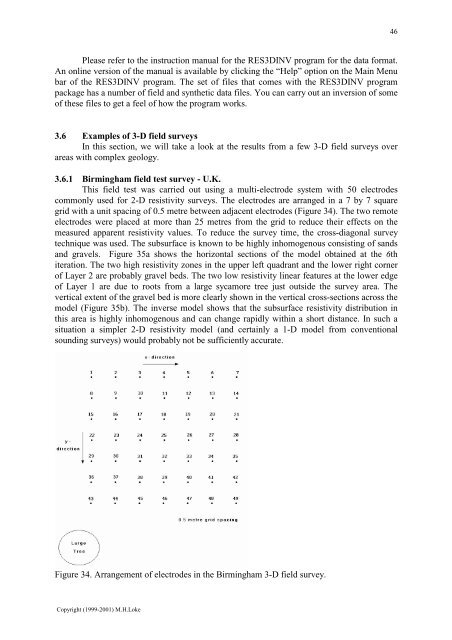
3.6.1 Birmingham field test survey - U.K.
This field test was carried out using a multi-electrode system with 50 electrodes
commonly used for 2-D resistivity surveys. The electrodes are arranged in a 7 by 7 square
grid with a unit spacing of 0.5 metre between adjacent electrodes (Figure 34). The two remote
electrodes were placed at more than 25 metres from the grid to reduce their effects on the
measured apparent resistivity values. To reduce the survey time, the cross-diagonal survey
technique was used. The subsurface is known to be highly inhomogenous consisting of sands
and gravels. Figure 35a shows the horizontal sections of the model obtained at the 6th
iteration. The two high resistivity zones in the upper left quadrant and the lower right corner
of Layer 2 are probably gravel beds. The two low resistivity linear features at the lower edge
of Layer 1 are due to roots from a large sycamore tree just outside the survey area. The
vertical extent of the gravel bed is more clearly shown in the vertical cross-sections across the
model (Figure 35b). The inverse model shows that the subsurface resistivity distribution in
this area is highly inhomogenous and can change rapidly within a short distance. In such a
situation a simpler 2-D resistivity model (and certainly a 1-D model from conventional
sounding surveys) would probably not be sufficiently accurate.
Figure 34. Arrangement of electrodes in the Birmingham 3-D field survey.
Copyright (1999-2001) M.H.Loke