THE SOLUTION OF COUPLED MODIFIED KDV SYSTEM BY THE ...

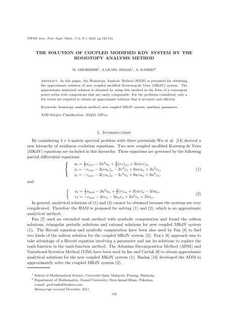
TWMS Jour. Pure Appl. Math., V.3, N.1, 2012, pp.122-134
THE SOLUTION OF COUPLED MODIFIED KDV SYSTEM BY THE
HOMOTOPY ANALYSIS METHOD
M. GHOREISHI 1 , A.I.B.MD. ISMAIL 1 , A. RASHID 2
Abstract. In this paper, the Homotopy Analysis Method (HAM) is presented for obtaining
the approximate solution of new coupled modified Korteweg-de Vries (MKdV) system. The
approximate analytical solution is obtained by using this method in the form of a convergent
power series with components that are easily computable. For the problems considered, only a
few terms are required to obtain an approximate solution that is accurate and efficient.
Keywords: homotopy analysis method, new coupled MKdV system, auxiliary parameter.
AMS Subject Classification: 35Q53, 55Pxx.
1. Introduction
By considering 4 × 4 matrix spectral problem with three potentials Wu et al. [14] derived a
new hierarchy of nonlinear evolution equations. Two new coupled modified Koreweg-de Vries
(MKdV) equations are included in this hierarchy. These equations are governed by the following
partial differential equations:
and
⎧
⎨
⎩
u t = 1 2 u xxx − 3u 2 u x + 3 2 (vz) xx + 3(uvz) x ,
v t = −v xxx − 3(vu x ) x − 3v 2 z x + 6uvu x + 3u 2 v x ,
z t = −z xxx − 3(zu x ) x − 3z 2 v x + 6uzu x + 3u 2 z x ,
{
ut = 1 2 u xxx − 3u 2 u x + 3 2 (v) xx + 3(uv) x − 3λu x ,
v t = −v xxx − 3vv x − 3u x v x + 3u 2 v x + 3λv x .
In general, analytical solutions of (1) and (2) cannot be obtained because the systems are very
complicated. Therefore the HAM is proposed for solving (1) and (2), which is an approximate
analytical method.
Fan [7] used an extended tanh method with symbolic computation and found the soliton
solutions, triangular periodic solutions and rational solutions for new coupled MKdV system
(1). The Riccati equation and symbolic computation have been also used by Fan [8] to find
two kinds of the soliton solution for the coupled MKdV system (2). Fan’s [8] approach was to
take advantage of a Riccati equation involving a parameter and use its solutions to replace the
tanh-function in the tanh-function method. The Adomian Decomposition Method (ADM) and
Variational Iteration Method (VIM) have been used by Inc and Cavlak [9] to obtain approximate
analytical solutions for the new coupled MKdV system (1). Raslan [13] developed the ADM to
approximately solve the coupled MKdV system (2).
(1)
(2)
1 School of Mathematical Science, Universiti Sains Malaysia, Penang, Malaysia,
2 Department of Mathematics, Gomal University, Dera Ismail Khan, Pakistan,
e-mail: prof.rashid@yahoo.com
Manuscript received December 2011.
122

M. GHOREISHI, A.I.B.MD. ISMAIL, A. RASHID: COUPLED MODIFIED KDV SYSTEM ... 123
The basic aim of this study is to obtain the approximate analytical solution for the coupled
system (1) and (2) using HAM. Approximate analytical schemes such as ADM, VIM, Homotopy
Perturbation Method (HPM) and HAM have been widely used to solve operator equations.
These schemes generate an infinite series solution and do not have the problem of rounding
error. The solution obtained by using these methods show their applicability, accuracy and
efficiency in solving many nonlinear problems in physics, engineering and various branches of
mathematics [12].
The HAM was developed by Liao [10] who utilized the idea of homotopy in topology. Since
then numerous authors have used HAM to solve various differential equations but as far as we
are aware systems (1) and (2) have not been solved by HAM. HAM has an advantage over
perturbation methods that it does not depend on small or large parameters. Compared with
other analytical methods such as ADM, VIM, HAM allows for fine-tuning of convergence region
and rate of convergence by allowing an auxiliary parameter to vary [1, 6].
This paper is organized as follows: In section 2, we present a description of the HAM, which
has been described by others, in particular [2, 3, 5]. In section 3, we employ the HAM for solving
two examples of the new coupled MKdV systems (1) and (2) and compare the approximate
solution obtained with the exact solution. Finally, in section 4, we give the conclusions of the
study.
2. A description of the HAM
To apply the HAM, the new coupled MKdV system (1) is considered. The following deformation
equation was constructed by Liao [10]
(1 − p)L u [φ(x, t; p) − u 0 (x, t)] = pH 1 (x, t)N 1 [φ(x, t; p)], (3)
(1 − p)L v [ϕ(x, t; p) − v 0 (x, t)] = pH 2 (x, t)N 2 [ϕ(x, t; p)], (4)
(1 − p)L z [ψ(x, t; p) − z 0 (x, t)] = pH 3 (x, t)N 3 [ψ(x, t; p)], (5)
where N 1 , N 2 and N 3 are three nonlinear operators, x and t denote the independent variables,
H 1 (x, t), H 2 (x, t) and H 3 (x, t) are auxiliary function, p ∈ [0, 1] is the embedding parameter,
≠ 0 is an auxiliary parameter, u 0 (x, t), v 0 (x, t) and z 0 (x, t) are initial guesses of u(x, t), v(x, t)
and z(x, t), respectively. The functions φ(x, t; p), ϕ(x, t; p) and ψ(x, t; p) are known functions
and L u , L v and L z are auxiliary operators that are defined as follows
which satisfies
L u [u(x, t)] = ∂u
∂t ,
L v[v(x, t)] = ∂v
∂t ,
L z[z(x, t)] = ∂z
∂t ,
L u [c 1 (x)] = 0, L v [c 2 (x)] = 0, L z [c 3 (x)] = 0,
where c 1 (x), c 2 (x) and c 3 (x) are integral constants. When p = 0 and p = 1, we get
φ(x, t; 0) = u 0 (x, t),
ϕ(x, t; 0) = v 0 (x, t),
ψ(x, t; 0) = z 0 (x, t),
φ(x, t; 1) = u(x, t),
ϕ(x, t; 1) = v(x, t),
ψ(x, t; 1) = z(x, t).
Hence as p increase from 0 to 1, the solution of coupled MKdV system (1) will vary from
the initial guesses u 0 (x, t), v 0 (x, t) and z 0 (x, t) to the exact solution u(x, t), v(x, t) and z(x, t).
Expanding φ(x, t; p), ϕ(x, t; p) and ψ(x, t; p) as a Taylor series with respect to p, gives
φ(x, t; p) = φ(x, t; 0) +
∞∑
m=1
p m ∂ m φ(x, t; p)
m! ∂p m | p=0 ,

124 TWMS JOUR. PURE APPL. MATH., V.3, N.1, 2012
Thus
where
ϕ(x, t; p) = ϕ(x, t; 0) +
ψ(x, t; p) = ψ(x, t; 0) +
∞∑
m=1
∞∑
m=1
φ(x, t; p) = u 0 (x, t) +
ϕ(x, t; p) = v 0 (x, t) +
ψ(x, t; p) = z 0 (x, t) +
p m ∂ m ϕ(x, t; p)
m! ∂p m | p=0 ,
p m ∂ m ψ(x, t; p)
m! ∂p m | p=0 .
∞∑
u m (x, t)p m , (6)
m=1
∞∑
v m (x, t)p m , (7)
m=1
∞∑
z m (x, t)p m , (8)
m=1
u m (x, t) = 1 ∂ m φ(x, t; p)
m! ∂p m | p=0 , (9)
v m (x, t) = 1 ∂ m ϕ(x, t; p)
m! ∂p m | p=0 , (10)
z m (x, t) = 1 ∂ m ψ(x, t; p)
m! ∂p m | p=0 . (11)
According to [4], the suitable choice of the initial condition u 0 (x, t), v 0 (x, t) and z 0 (x, t), the
auxiliary linear parameter L u , L v and L z , the non-zero auxiliary parameter and the auxiliary
function H 1 (x, t), H 2 (x, t) and H 3 (x, t) will guarantee that
(1) The solution φ(x, t; p), ϕ(x, t; p) ψ(x, t; p) of the zero-order deformation equation (3)-(5)
exists for all p ∈ [0, 1].
(2) The deformation derivative ∂m φ(x, t; p)
∂p m | p=0 , ∂m ϕ(x, t; p)
∂p m | p=0 and ∂m ψ(x, t; p)
∂p m | p=0 exists
for m = 1, 2, . . . .
(3) The power series (6)-(8) converges at p = 1.
If p = 1
φ(x, t; 1) = u(x, t) = u 0 (x, t) +
ϕ(x, t; 1) = v(x, t) = v 0 (x, t) +
ψ(x, t; 1) = z(x, t) = z 0 (x, t) +
∞∑
u m (x, t), (12)
m=1
∞∑
v m (x, t), (13)
m=1
∞∑
z m (x, t), (14)
which must be one of the solutions of new coupled MKdV system (1). According to the definition
(9)-(11), the governing equations can be deduced from the (zero-order deformation) equations
(3)-(5). For further analysis, the vectors
m=1
⃗u n (x, t) = {u 0 (x, t), u 1 (x, t), . . . , u n (x, t)},
⃗v n (x, t) = {v 0 (x, t), v 1 (x, t), . . . , v n (x, t)},
⃗z n (x, t) = {z 0 (x, t), z 1 (x, t), . . . , z n (x, t)},

M. GHOREISHI, A.I.B.MD. ISMAIL, A. RASHID: COUPLED MODIFIED KDV SYSTEM ... 125
are defined. Differentiating equations (3)-(5) m-times with respect to the parameter p and then
dividing by m! and setting p = 0, gives the linear equations [10]
with the initial conditions
where
and we have
L u [u m (x, t) − χ m u m−1 (x, t)] = R 1m (⃗u m−1 ), (15)
L v [v m (x, t) − χ m v m−1 (x, t)] = R 2m (⃗v m−1 ), (16)
L z [z m (x, t) − χ m z m−1 (x, t)] = R 3m (⃗z m−1 ), (17)
R 1m (u m−1 ) =
R 2m (v m−1 ) =
R 3m (z m−1 ) =
u m (x, 0) = 0,
v m (x, 0) = 0,
z m (x, 0) = 0,
1
(m − 1)! × ∂m−1 N 1 (φ(x, t; p))
∂p m−1 , (18)
1
(m − 1)! × ∂m−1 N 2 (ϕ(x, t; p))
∂p m−1 , (19)
1
(m − 1)! × ∂m−1 N 3 (ψ(x, t; p))
∂p m−1 , (20)
χ m =
{
0, m ≤ 1,
1, m > 1.
Now, the solution of the m-order deformation equations (15)-(17) for m ≥ 1 becomes
u m (x, t) = χ m u m−1 (x, t) +
v m (x, t) = χ m v m−1 (x, t) +
z m (x, t) = χ m z m−1 (x, t) +
∫ t
0
∫ t
0
∫ t
0
H 1 (x, t)R 1m (⃗u m−1 )dt, (21)
H 2 (x, t)R 2m (⃗v m−1 )dt, (22)
H 3 (x, t)R 3m (⃗z m−1 )dt. (23)
The detailed analysis of the convergence of the HAM is discussed by Liao in [11]. We note
that the HAM only utilities the initial and makes no use of the boundary conditions.
3. Numerical solutions
In this section, the HAM will be demonstrated on examples of new coupled MKdV. For our
numerical computation, let the expression
ψ m (x, t) =
m−1
∑
k=0
u k (x, t), (24)
denote the m-term HAM approximation to u(x, t). We compare the approximate analytical
solution is obtained using HAM for our new coupled MKdV with the exact solution. We define
E m (x, t) to be the absolute error between the exact solution and m-term approximate HAM
solution ψ m (x, t) as follows
E m (x, t) = |u(x, t) − ψ m (x, t)|. (25)

126 TWMS JOUR. PURE APPL. MATH., V.3, N.1, 2012
Example 3.1. For the first example, we present the new coupled MKdV equations with analytical
solution to show the efficiency of HAM, which has been described in the section 2. We consider
the system (1) with initial conditions as follows [7, 9]
u(x, 0) = 1 + 1 tanh x,
2
v(x, 0) = 1 2 − 1 tanh x,
4
z(x, 0) = 2 − tanh x.
It can be verified that the exact solutions of this example are
u(x, t) = 1 + 1 (
2 tanh x − 11 )
2 t ,
v(x, t) = 1 2 − 1 (
4 tanh x − 11 )
2 t ,
(
z(x, t) = 2 − tanh x − 11 )
2 t .
We start with the following zeroth-components
u 0 (x, t) = 1 + 1 tanh x, (26)
2
v 0 (x, t) = 1 2 − 1 tanh x,
4
(27)
z 0 (x, t) = 2 − tanh x. (28)
According to section 2, we can define the operators N 1 , N 2 and N 3 as
N 1 [φ] = φ t − 1 2 φ xxx + 3φ 2 φ x − 3 2 (ϕψ) xx − 3(φϕψ) x , (29)
N 2 [ϕ] = ϕ t + ϕ xxx + 3(ϕφ x ) x + 3ϕ 2 ψ x − 6φϕφ x − 3φ 2 ϕ x , (30)
N 3 [ψ] = ψ t + ψ xxx + 3(ψφ x ) x + 3ψ 2 ϕ x − 6φψφ x − 3φ 2 ψ x , (31)
Now, we can obtain the zeroth-
where φ = φ(x, t; p), ϕ = ϕ(x, t; p) and ψ = ψ(x, t; p).
deformation equation (15)-(17) as
(
R 1m (⃗u m−1 ) = (u m−1 ) t − 1 2 (u m−1) xxx + 3
− 3 2
( m−1
)
∑
v i z m−1−i −
i=0
xx
R 2m (⃗v m−1 ) = (v m−1 ) t + (v m−1 ) xxx +3
+3
m−1
∑
i=0
(
∑
v i
m−1−i
k=0
v k (z m−1−i−k ) x
)
−6
−3
m−1
∑
i=0
( m−1 ∑
i=0
∑
u i
m−1−i
k=0
∑
u i
m−1−i
k=0
( m−1
)
∑
v i (u m−1−i ) x
i=0
m−1
∑
i=0
m−1
∑
i=0
(
(
∑
u i
m−1−i
k=0
∑
u i
m−1−i
k=0
u k (u m−1−i−k ) x
)
−
(v k z m−1−i−k )
x
+
)
v k (u m−1−i−k ) x
)
−
u k (v m−1−i−k ) x
)
,
x
,
(32)
(33)

and
M. GHOREISHI, A.I.B.MD. ISMAIL, A. RASHID: COUPLED MODIFIED KDV SYSTEM ... 127
R 3m (⃗z m−1 ) = (z m−1 ) t + (z m−1 ) xxx +3
+3
m−1
∑
i=0
(
∑
z i
m−1−i
k=0
z k (v m−1−i−k ) x
)
−6
−3
( m−1
)
∑
z i (u m−1−i ) x
i=0
m−1
∑
i=0
m−1
∑
i=0
(
(
∑
u i
m−1−i
k=0
∑
u i
m−1−i
k=0
x
+
z k (u m−1−i−k ) x
)
−
u k (z m−1−i−k ) x
)
We start with the initial conditions (26)-(28). By means of the (21)-(23), we can obtain directly
the other components of the HAM solution in the series form of (12)-(14). Thus, we have
and
u 1 (x, t) = t(−3( 1 2 sec h2 x(2 − tanh x)( 1 2 − tanh x
4
−sech 2 x( 1 2 − tanh x
4
v 1 (x, t) = t(−3 sec h 2 x( 1 2 − tanh x
4
×(1 + tanh x
2
)(1 + tanh x
2
) − 1 4 sec h2 x(2 − tanh x)(1 + tanh x )−
2
)) + 3 2 sec h2 x(1 + tanh x ) − 3 2 2 (sec h4 x
+ . . .
2
) 2 − 3 sec h 2 x( 1 2 − tanh x
4
)(1 + tanh x ) + 3 2 4 sec h2 x×
) 2 + 4(− 1 8 sec h4 x − sec h 2 x( 1 2 − tanh x ) tanh x) + 1 4
4 (2 sec h4 x − 4 sec h 2 x . . .
z 1 (x, t) = t(2 sec h 4 x − 3 4 sec h2 x(2 − tanh x) 2 − 3 sec h 2 x(2 − tanh x)(1 + tanh x ) + 3 sec h 2 x×
2
×(1 + tanh x ) 2 − 4 sec h 2 x tanh 2 x + 3(− 1 2
2 sec h4 x − sec h 2 x(2 − tanh x) tanh x.
and so on. Thus u(x, t) and v(x, t) can be written as follows
∞∑
u(x, t) = u n (x, t) = u 0 (x, t) + u 1 (x, t) + u 2 (x, t) + . . . ,
v(x, t) =
n=0
∞∑
v n (x, t) = v 0 (x, t) + v 1 (x, t) + v 2 (x, t) + . . . .
n=0
Table 1, 2 and 3 show the absolute error between solution obtained using HAM with five terms
and the exact solution for u(x, t), v(x, t) and z(x, t), respectively, at = −0.72. The errors are
very small in these tables. The results show that the homotopy analysis method is very useful
to obtain explicit approximate analytical solutions. A very good approximation with the actual
solution of the equations were achieved by using five terms only. We have ascertained that the
overall errors can be made smaller by adding new terms of the HAM series (12)-(14).
Table 1: Absolute error E 5 for variables x and t at = −0.72 for u(x, t).
t/x -15 -10 10 15
0.1 0. 1.53949×10 −12 1.98090×10 −10 8.77076×10 −15
0.2 9.54792×10 −15 2.12719×10 −10 3.17572×10 −9 1.43996×10 −13
0.3 3.65263×10 −14 8.06111×10 −10 2.15028×10 −8 9.76219×10 −13
0.4 5.76206×10 −14 1.26782×10 −10 9.99208×10 −8 4.53626×10 −12
0.5 6.43929×10 −15 1.40508×10 −10 3.81990×10 −7 1.73420×10 −11
.
(34)

128 TWMS JOUR. PURE APPL. MATH., V.3, N.1, 2012
Table 2: Absolute error E 5 for variables x and t at = −0.72 for v(x, t).
t/x -15 -10 10 15
0.1 0. 1.67374×10 −12 3.17747×10 −10 1.44329×10 −14
0.2 4.55191×10 −15 1.00864×10 −10 5.46088×10 −10 2.47580×10 −14
0.3 1.90840×10 −14 4.39246×10 −10 5.37478×10 −9 2.43972×10 −13
0.4 3.98570×10 −14 8.78399×10 −10 4.02239×10 −8 1.82621×10 −12
0.5 3.99680×10 −14 8.80336×10 −10 1.76823×10 −7 8.02775×10 −12
Table 3: Absolute error E 5 for variables x and t at = −0.72 for z(x, t).
t/x -15 -10 10 15
0.1 0. 5.33562×10 −12 8.07505×10 −10 3.66374×10 −14
0.2 5.77816×10 −15 1.38055×10 −10 8.88212×10 −9 4.03233×10 −13
0.3 1.33227×10 −14 2.99971×10 −10 5.08123×10 −8 2.30660×10 −12
0.4 4.30767×10 −14 9.36929×10 −10 2.17691×10 −7 9.88321×10 −12
0.5 1.62537×10 −13 3.58345×10 −9 7.98407×10 −7 3.62477×10 −11
Absolute error u forħ⩵0.72 at x⩵15
Absolute error v forħ⩵0.72 at x⩵15
5.10 14 t
4.10 14 t
E5
4.10 14
3.10 14
2.10 14
1.10 14
0
0.0 0.1 0.2 0.3 0.4 0.5
E5
3.10 14
2.10 14
1.10 14
0
0.0 0.1 0.2 0.3 0.4 0.5
Figure 1. The absolute error between HAM solution and the exact solution for = −0.72 at x = −15.
Absolute error u forħ⩵0.72 at x⩵15
1.510 13 t
1.10 13
E5
5.10 14
0
0.0 0.1 0.2 0.3 0.4 0.5
Figure 2. The absolute error between HAM solution and the exact solution for = −0.72 at x = −15.
In figure 1 and 2, the absolute error between solution obtained using HAM with five terms and
the exact solution have been plotted for u(x, t), v(x, t) and z(x, t) for case of = −0.72 at
x = −15. Similarly, we show this error in figure 3 and 4 at x = 15. In figure 5 and 6, we have
shown the -curve for u t (0, 0), v t (0, 0) and z t (0, 0). As we know, the auxiliary parameter can
be employed to adjust the convergence region of the homotopy analysis solution [11]. According
to these -curve, it is easy to discover the valid region of which corresponds to the line segment

M. GHOREISHI, A.I.B.MD. ISMAIL, A. RASHID: COUPLED MODIFIED KDV SYSTEM ... 129
nearly parallel to the horizontal axis. From figures 5 and 6, it is clear that the HAM series is
convergent when −1.4 < < −0.6.
Absolute error u forħ⩵0.72 at x⩵15
Absolute error u forħ⩵0.72 at x⩵15
1.10 11 t
4.10 12 t
E5
8.10 12
6.10 12
4.10 12
2.10 12
0
0.0 0.1 0.2 0.3 0.4 0.5
E5
3.10 12
2.10 12
1.10 12
0
0.0 0.1 0.2 0.3 0.4 0.5
Figure 3. The absolute error between HAM solution and the exact solution for = −0.72 at x = 15.
Absolute error u forħ⩵0.72 at x⩵15
2.10 11 t
1.510 11
E5
1.10 11
5.10 12
0
0.0 0.1 0.2 0.3 0.4 0.5
Figure 4. The absolute error between HAM solution and the exact solution for = −0.72 at x = 15.
ħcurve for u t 0,0
20
15
u t 0,0
10
5
0
2.0 1.5 1.0 0.5 0.0 0.5 1.0
ħ
Figure 5. The -curve for u t(0, 0) given by the 5-order HAM approximation solution when H 1(x, t) = 1.

130 TWMS JOUR. PURE APPL. MATH., V.3, N.1, 2012
ħcurve for v t 0,0
ħcurve for z t 0,0
0
0
2
2
4
4
v t 0,0
6
8
z t 0,0
6
8
10
10
12
12
2.0 1.5 1.0 0.5 0.0 0.5 1.0
ħ
2.0 1.5 1.0 0.5 0.0 0.5 1.0
ħ
Figure 6. The -curve for v t(0, 0) and z t(0, 0) given by the 5-order HAM approximation solution when
H 2 (x, t) = H 3 (x, t) = 1.
Example 3.2. Consider the coupled MKdV equation (2) with the initial conditions [8, 13]
u(x, 0) = k tanh(kx),
v(x, 0) = 1 2 (4k2 + λ) − 2k 2 tanh 2 (kx).
It can be verified that the exact solutions of this system are
(
u(x, t) = k tanh kx − k )
2 (2k2 + 3λ)t ,
v(x, t) = 1 2 (4k2 + λ) − 2k 2 tanh
(kx 2 − k )
2 (2k2 + 3λ)t .
We start with the initial conditions
u 0 (x, t) = k tanh(kx), (35)
v 0 (x, t) = 1 2 (4k2 + λ) − 2k 2 tanh 2 (kx). (36)
According to section 2, we can define the operators N 1 and N 2 as
N 1 [φ] = φ t − 1 2 φ xxx + 3φ 2 φ x − 3 2 (ϕ) xx − 3(φϕ) x + 3λφ x (37)
N 2 [ϕ] = ϕ t + ϕ xxx + 3ϕϕ x + 3φ x ϕ x − 3φ 2 ϕ x − 3λϕ x , (38)
where φ = φ(x, t; p) and ϕ = ϕ(x, t; p).
equation (15) and (16) that are
Now, we can obtain the zeroth-order deformation
R 1m (⃗u m−1 ) = (u m−1 ) t − 1 2 (u m−1) xxx + 3
− 3 2 (v m−1) xx − 3
m−1
∑
i=0
(
∑
u i
m−1−i
k=0
( m−1
)
∑
(u i v m−1−i )
i=0
u k (u m−1−i−k ) x
)
−
x
+ 3λ(u m−1 ) x ,
(39)

M. GHOREISHI, A.I.B.MD. ISMAIL, A. RASHID: COUPLED MODIFIED KDV SYSTEM ... 131
and
R 2m (⃗v m−1 ) = (v m−1 ) t + (v m−1 ) xxx +3
( m−1
) ( ∑ m−1
) ∑
v i (v m−1−i ) x + 3 (u i ) x (v m−1−i ) x −
i=0
i=0
∑
m−1
−3
i=0
( m−1−i
) ∑
u i u k (v m−1−i−k ) x − 3λ(v m−1 ) x .
k=0
(40)
We start with the initial conditions (35) and (36). By means of the (21) and (22), we can
easily obtain directly the other component of the HAM solution in the series form of (12) and
(13). Thus, we have
u 1 (x, t) = t[3λk 2 sec h 2 (kx) + 3k 4 sec h 2 (kx) tanh 2 (kx) + 3k 2 (2k 2 sec h 4 (kx) − 4k 2 sec h 2 (kx)×
× tanh 2 (kx) − k 2 (−2k3 sec h 4 (kx) + 4k 3 sec h 2 (kx) tanh 2 (kx)) − 3(−4k 2 sec h 2 (kx)×
× tanh 2 (kx) + k 2 sec h 2 (kx)( 1 2 (λ + 4k2 ) − 2k 2 tanh 2 (kx))))].
v 1 (x, t) = t[12λk 3 sec h 2 (kx) tanh(kx) − 12k 5 sec h 4 (kx) tanh(kx) + 12k 5 sec h 2 (kx) tanh 3 (kx)−
−12 sec h 2 (kx) tanh(kx)( 1 2 (4k2 + λ) − 2k 2 tanh 2 (kx)) − 2k 2 (−16k 3 sec h 4 (kx)×
× tanh(kx) + 8k 3 sec h 2 (kx) tanh 3 (kx))]
and so on. Thus u(x, t) and v(x, t) can be written as follows
u(x, t) =
v(x, t) =
∞∑
u n (x, t) = u 0 (x, t) + u 1 (x, t) + u 2 (x, t) + . . . ,
n=0
∞∑
v n (x, t) = v 0 (x, t) + v 1 (x, t) + v 2 (x, t) + . . . .
n=0
Table 4 and 5 show the absolute error between solution obtained using HAM with four terms
and the exact solution for u(x, t) and v(x, t), respectively, at = −1, k = 0.1 and λ = 0.1. The
errors are very small in these tables. The results show that the homotopy analysis method is
very useful to obtain explicit approximate analytical solutions. A very good approximation with
the actual solution of the equations was achieved by using four terms only. We have ascertained
that the overall errors can be made smaller by adding new terms of the HAM series (12) and
(13).
Table 4: Absolute error E 4 for variables x and t at = −1, for u(x, t).
x/t 0.1 0.2 0.3 0.4
-100 1.24447×10 −19 1.13618×10 −17 5.58676×10 −18 1.01850×10 −17
-40 6.46940×10 −13 2.59019×10 −12 5.83872×10 −12 1.04084×10 −11
-10 4.83626×10 −8 1.93467×10 −7 4.35339×10 −7 7.74002×10 −7
10 4.83541×10 −8 1.93399×10 −7 4.35109×10 −7 7.73457×10 −7
40 6.47442×10 −13 2.59443×10 −12 5.85271×10 −12 1.04417×10 −11
100 2.51949×10 −18 6.81357×10 −18 6.13444×10 −19 7.00450×10 −18

132 TWMS JOUR. PURE APPL. MATH., V.3, N.1, 2012
Absolute error u forħ⩵1, k⩵0.1,Λ⩵0.1 at x⩵100
Absolute error u forħ⩵1, k⩵0.1,Λ⩵0.1 at x⩵100
1.410 17 t
4.10 12 t
1.210 17
1.10 17
3.10 12
E4
8.10 18
6.10 18
E4
2.10 12
4.10 18
1.10 12
2.10 18
0
0.0 0.1 0.2 0.3 0.4
0
0.0 0.1 0.2 0.3 0.4
Figure 7. The absolute error E 4 for = −1, k = 0.1, λ = 0.1 at x = −100.
Absolute error u forħ⩵1, k⩵0.1,Λ⩵0.1 at x⩵0
Absolute error u forħ⩵1, k⩵0.1,Λ⩵0.1 at x⩵0
2.10 9 t
1.510 9
E4
1.10 9
E4
1.510 7 t
1.10 7
5.10 10
5.10 8
0
0.0 0.1 0.2 0.3 0.4
0
0.0 0.1 0.2 0.3 0.4
Figure 8. The absolute error E 4 for = −1, k = 0.1, λ = 0.1 at x = 0.
0.05
ħcurve for u t 0,0
0.0010
ħcurve for v t 0.5,0
0.04
0.0008
0.03
0.0006
u t 0,0
0.02
0.01
v t 0.5,0
0.0004
0.0002
0.00
0.0000
0.01
0.0002
2.0 1.5 1.0 0.5 0.0 0.5 1.0
ħ
2.0 1.5 1.0 0.5 0.0 0.5 1.0
ħ
Figure 9. The -curve for u t (0, 0) and v t (0.5, t) given by the 4th-order HAM approximation solution when
H 1(x, t) = H 2(x, t) = 1.

M. GHOREISHI, A.I.B.MD. ISMAIL, A. RASHID: COUPLED MODIFIED KDV SYSTEM ... 133
Table 5: Absolute error E 4 for variables x and t at = −1, for v(x, t).
x/t 0.1 0.2 0.3 0.4
-100 9.89160×10 −13 1.97793×10 −12 2.96632×10 −12 3.95434×10 −12
-40 1.60774×10 −7 3.21486×10 −7 4.82137×10 −7 6.42728×10 −7
-10 3.83856×10 −5 7.67786×10 −5 1.15179×10 −4 1.53586×10 −4
10 3.83784×10 −5 7.67495×10 −5 1.15113×10 −4 1.53470×10 −4
40 1.60838×10 −7 3.21742×10 −7 4.82713×10 −7 6.43752×10 −7
100 9.89547×10 −13 1.97951×10 −12 2.96988×10 −12 3.96067×10 −12
In figures 7 and 8, we have displayed the absolute error between solution obtained using HAM
with four terms and the exact solution for = −1, k = 0.1, λ = 0.5 at x = −100 and x = 0,
respectively. The -curves have been plotted in figure 9 for u t (0, 0) and v t (0.5, t). As we have
expressed, it is easy to check that the HAM solution is convergent to the exact solutions when
−1.4 < < −0.6.
4. Conclusion
In this paper, we have illustrated how HAM can be used for the new coupled modification
of KdV system. The method was tested on two examples. The HAM solution contains the
auxiliary parameter ≠ 0 provides a method to adjust and control the convergence region of
the infinite series for large value of t. The obtained results show that the HAM is a very accurate
and effective technique for the solution of the new MKdV system.
References
[1] Alomari, A.K., Noorani, M.S.M., Nazar, R., Li, C.P., (2010), Homotopy analysis method for solving fractional
Lorenz system, Communications in Nonlinear Science and Numerical Simulation, 15, pp.1864–1872.
[2] Alomari, A. K., Noorani, M. S. M., Nazar, R.,(2009), Comparison between the homotopy analysis method
and homotopy paerturbation method to solve coupled Schrodinger-KdV equation, Journal of Applied Mathematics
and Computation, 31, pp.1–12.
[3] Alomari, A.K., Noorani, M.S.M., Nazar, R., (2008), The homotopy analysis method for the exact solutions
of the K(2,2), Burgers and coupled Burgers equations, Applied Mathematical Sciences, 2(40), pp.1963–1977.
[4] Awawdeh, F., Adawi, A., Mustafa, Z., (2009), Solutions of the SIR models of epidemics using HAM, Chaos,
Solitons and Fractals, 42, pp.3047–3052.
[5] Bataineh, A.S., Noorani, M.S.M., Hashim, I., (2009), On a new reliable modification of homotopy analysis
method, Communications in Nonlinear Science and Numerical Simulation, 14, pp.409–423.
[6] Bataineh, A.S., Noorani, M.S.M., Hashim, I., (2009), Modified homotopy analysis method for solving systems
of second-order BVPs, Communications in Nonlinear Science and Numerical Simulation, 14, pp.430–442.
[7] Fan, E., (2002), Using symbolic computation to exactly solve a new coupled MKdV system, Physics Letter
A, 299(1), pp.46–48.
[8] Fan, E., (2001), Soliton solutions for a generalized HirotaSatsuma coupled KdV equation and a coupled
MKdV equation, Physics Letters A, 282, pp.18–22.
[9] Inc, M., Cavlak, E., (2008), On numerical solutions of a new coupled MKdV system by using the Adomian
decomposition method and He’s variational iteration method, Physica Scripta, 78, pp.1–7.
[10] Liao, S.-J., (1992), The Proposed Homotopy Analysis Techniques for the Solution of Nonlinear Problems,
Ph.D.dissertation, Shanghai Jiao Tong University, Shanghai, China.
[11] Liao, S.-J., (2003), Beyond Perturbation: Introduction to the Homotopy Analysis Method, CRC Press, Boca
Raton, Chapman and Hall.
[12] Rashid, A., Izani, A.M.I., (2010), A Chebyshev spectral collocation method for the coupled nonlinear
Schrdinger equations, International Journal of Applied and Computational Mathematics, 9(1), pp.104–115
[13] Raslan, K.R., (2004), The decomposition method for a Hirota-Satsuma coupled KdV equation and a coupled
MKdV equation, International Journal of Computer Mathematics, 81(12), pp.1497–1505.

134 TWMS JOUR. PURE APPL. MATH., V.3, N.1, 2012
[14] Wu, Y.T., Geng, X.G., Hu, X.B., Zhu, S., (1999), A generalized HirotaSatsuma coupled Kortewegde Vries
equation and Miura transformations, Physics Letters A, 255(4-6), pp.259–264.
Seyed Mohammad Ghoreishi was born in
Tehran-Iran. He obtained his B.Sc. from University
of Sistan and Baluchestan in 1994. He received
his M. Sc. from University of Science and Technology,
Iran in 1997. He worked as a lecturer at several
Universities of Iran in 1997 to 2007. He received his
Ph.D. in Applied Mathematics from School of Mathematical
Sciences, Universiti Sains Malaysia, Penang,
Malaysia in 2011. He studied the numerical and approximate
analytical solution of parabolic equations
with nonlocal boundary conditions.
Ahmad Izani Md. Ismail joined the School of
Mathematical Sciences, Universiti Sains Malaysia, in
1984 and was appointed a Professor in 2011. He has
taught undergraduate and graduate courses on numerical
analysis, mathematical modeling, fluid mechanics
and computer programming. His primary research
interest is in mathematical modeling and he
is presently supervising and co-supervising 8 Ph.D.
students.
Abdur Rashid joined the Department of Mathematics,
Gomal University, Dera Ismail Khan, Pakistan
in 1983. He completed Ph.D. from Shanghai
University of Science Technology, Shanghai, P. R.
China, in 1993. He was appointed a Professor at Department
of Mathematics, Gomal University, Dera Ismail
Khan, Pakistan, in 2008. His research interest is
Numerical Solution of Partial Differential Equations
by Spectral methods.