THE SOLUTION OF COUPLED MODIFIED KDV SYSTEM BY THE ...

and
M. GHOREISHI, A.I.B.MD. ISMAIL, A. RASHID: COUPLED MODIFIED KDV SYSTEM ... 127
R 3m (⃗z m−1 ) = (z m−1 ) t + (z m−1 ) xxx +3
+3
m−1
∑
i=0
(
∑
z i
m−1−i
k=0
z k (v m−1−i−k ) x
)
−6
−3
( m−1
)
∑
z i (u m−1−i ) x
i=0
m−1
∑
i=0
m−1
∑
i=0
(
(
∑
u i
m−1−i
k=0
∑
u i
m−1−i
k=0
x
+
z k (u m−1−i−k ) x
)
−
u k (z m−1−i−k ) x
)
We start with the initial conditions (26)-(28). By means of the (21)-(23), we can obtain directly
the other components of the HAM solution in the series form of (12)-(14). Thus, we have
and
u 1 (x, t) = t(−3( 1 2 sec h2 x(2 − tanh x)( 1 2 − tanh x
4
−sech 2 x( 1 2 − tanh x
4
v 1 (x, t) = t(−3 sec h 2 x( 1 2 − tanh x
4
×(1 + tanh x
2
)(1 + tanh x
2
) − 1 4 sec h2 x(2 − tanh x)(1 + tanh x )−
2
)) + 3 2 sec h2 x(1 + tanh x ) − 3 2 2 (sec h4 x
+ . . .
2
) 2 − 3 sec h 2 x( 1 2 − tanh x
4
)(1 + tanh x ) + 3 2 4 sec h2 x×
) 2 + 4(− 1 8 sec h4 x − sec h 2 x( 1 2 − tanh x ) tanh x) + 1 4
4 (2 sec h4 x − 4 sec h 2 x . . .
z 1 (x, t) = t(2 sec h 4 x − 3 4 sec h2 x(2 − tanh x) 2 − 3 sec h 2 x(2 − tanh x)(1 + tanh x ) + 3 sec h 2 x×
2
×(1 + tanh x ) 2 − 4 sec h 2 x tanh 2 x + 3(− 1 2
2 sec h4 x − sec h 2 x(2 − tanh x) tanh x.
and so on. Thus u(x, t) and v(x, t) can be written as follows
∞∑
u(x, t) = u n (x, t) = u 0 (x, t) + u 1 (x, t) + u 2 (x, t) + . . . ,
v(x, t) =
n=0
∞∑
v n (x, t) = v 0 (x, t) + v 1 (x, t) + v 2 (x, t) + . . . .
n=0
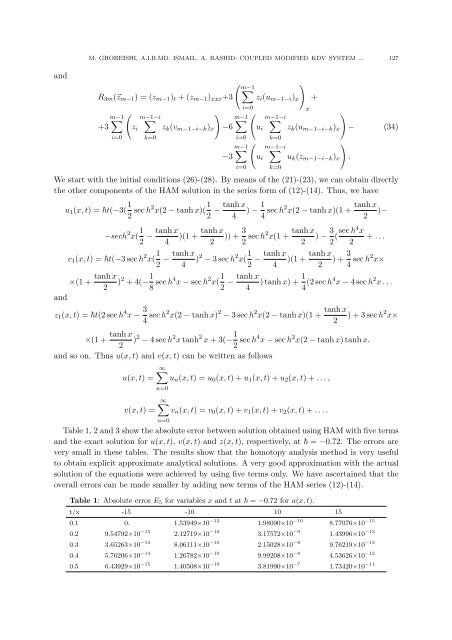
Table 1, 2 and 3 show the absolute error between solution obtained using HAM with five terms
and the exact solution for u(x, t), v(x, t) and z(x, t), respectively, at = −0.72. The errors are
very small in these tables. The results show that the homotopy analysis method is very useful
to obtain explicit approximate analytical solutions. A very good approximation with the actual
solution of the equations were achieved by using five terms only. We have ascertained that the
overall errors can be made smaller by adding new terms of the HAM series (12)-(14).
Table 1: Absolute error E 5 for variables x and t at = −0.72 for u(x, t).
t/x -15 -10 10 15
0.1 0. 1.53949×10 −12 1.98090×10 −10 8.77076×10 −15
0.2 9.54792×10 −15 2.12719×10 −10 3.17572×10 −9 1.43996×10 −13
0.3 3.65263×10 −14 8.06111×10 −10 2.15028×10 −8 9.76219×10 −13
0.4 5.76206×10 −14 1.26782×10 −10 9.99208×10 −8 4.53626×10 −12
0.5 6.43929×10 −15 1.40508×10 −10 3.81990×10 −7 1.73420×10 −11
.
(34)