THE SOLUTION OF COUPLED MODIFIED KDV SYSTEM BY THE ...
THE SOLUTION OF COUPLED MODIFIED KDV SYSTEM BY THE ...
THE SOLUTION OF COUPLED MODIFIED KDV SYSTEM BY THE ...

Create successful ePaper yourself
Turn your PDF publications into a flip-book with our unique Google optimized e-Paper software.
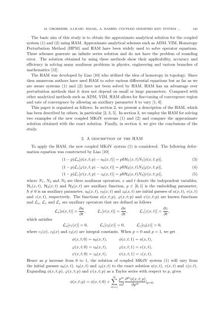
M. GHOREISHI, A.I.B.MD. ISMAIL, A. RASHID: <strong>COUPLED</strong> <strong>MODIFIED</strong> <strong>KDV</strong> <strong>SYSTEM</strong> ... 123<br />
The basic aim of this study is to obtain the approximate analytical solution for the coupled<br />
system (1) and (2) using HAM. Approximate analytical schemes such as ADM, VIM, Homotopy<br />
Perturbation Method (HPM) and HAM have been widely used to solve operator equations.<br />
These schemes generate an infinite series solution and do not have the problem of rounding<br />
error. The solution obtained by using these methods show their applicability, accuracy and<br />
efficiency in solving many nonlinear problems in physics, engineering and various branches of<br />
mathematics [12].<br />
The HAM was developed by Liao [10] who utilized the idea of homotopy in topology. Since<br />
then numerous authors have used HAM to solve various differential equations but as far as we<br />
are aware systems (1) and (2) have not been solved by HAM. HAM has an advantage over<br />
perturbation methods that it does not depend on small or large parameters. Compared with<br />
other analytical methods such as ADM, VIM, HAM allows for fine-tuning of convergence region<br />
and rate of convergence by allowing an auxiliary parameter to vary [1, 6].<br />
This paper is organized as follows: In section 2, we present a description of the HAM, which<br />
has been described by others, in particular [2, 3, 5]. In section 3, we employ the HAM for solving<br />
two examples of the new coupled MKdV systems (1) and (2) and compare the approximate<br />
solution obtained with the exact solution. Finally, in section 4, we give the conclusions of the<br />
study.<br />
2. A description of the HAM<br />
To apply the HAM, the new coupled MKdV system (1) is considered. The following deformation<br />
equation was constructed by Liao [10]<br />
(1 − p)L u [φ(x, t; p) − u 0 (x, t)] = pH 1 (x, t)N 1 [φ(x, t; p)], (3)<br />
(1 − p)L v [ϕ(x, t; p) − v 0 (x, t)] = pH 2 (x, t)N 2 [ϕ(x, t; p)], (4)<br />
(1 − p)L z [ψ(x, t; p) − z 0 (x, t)] = pH 3 (x, t)N 3 [ψ(x, t; p)], (5)<br />
where N 1 , N 2 and N 3 are three nonlinear operators, x and t denote the independent variables,<br />
H 1 (x, t), H 2 (x, t) and H 3 (x, t) are auxiliary function, p ∈ [0, 1] is the embedding parameter,<br />
≠ 0 is an auxiliary parameter, u 0 (x, t), v 0 (x, t) and z 0 (x, t) are initial guesses of u(x, t), v(x, t)<br />
and z(x, t), respectively. The functions φ(x, t; p), ϕ(x, t; p) and ψ(x, t; p) are known functions<br />
and L u , L v and L z are auxiliary operators that are defined as follows<br />
which satisfies<br />
L u [u(x, t)] = ∂u<br />
∂t ,<br />
L v[v(x, t)] = ∂v<br />
∂t ,<br />
L z[z(x, t)] = ∂z<br />
∂t ,<br />
L u [c 1 (x)] = 0, L v [c 2 (x)] = 0, L z [c 3 (x)] = 0,<br />
where c 1 (x), c 2 (x) and c 3 (x) are integral constants. When p = 0 and p = 1, we get<br />
φ(x, t; 0) = u 0 (x, t),<br />
ϕ(x, t; 0) = v 0 (x, t),<br />
ψ(x, t; 0) = z 0 (x, t),<br />
φ(x, t; 1) = u(x, t),<br />
ϕ(x, t; 1) = v(x, t),<br />
ψ(x, t; 1) = z(x, t).<br />
Hence as p increase from 0 to 1, the solution of coupled MKdV system (1) will vary from<br />
the initial guesses u 0 (x, t), v 0 (x, t) and z 0 (x, t) to the exact solution u(x, t), v(x, t) and z(x, t).<br />
Expanding φ(x, t; p), ϕ(x, t; p) and ψ(x, t; p) as a Taylor series with respect to p, gives<br />
φ(x, t; p) = φ(x, t; 0) +<br />
∞∑<br />
m=1<br />
p m ∂ m φ(x, t; p)<br />
m! ∂p m | p=0 ,