Improvement methods of reconstruction process in digital holography

More documents

Recommendations

Info

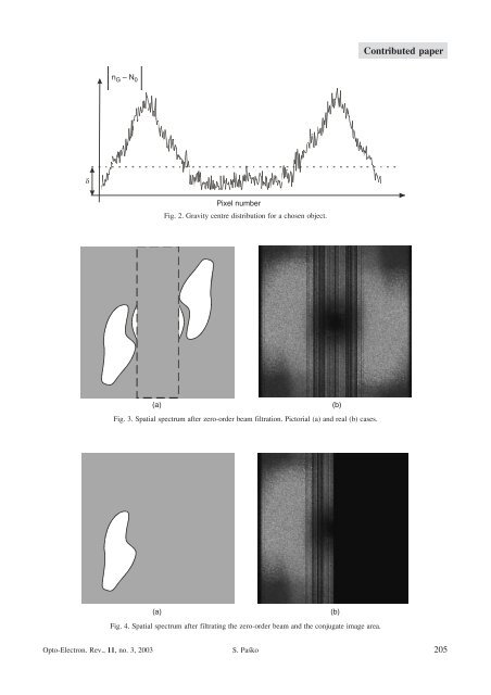
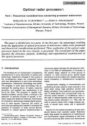
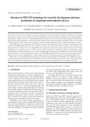
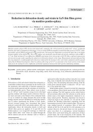
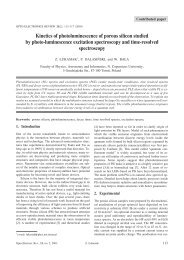
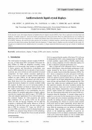
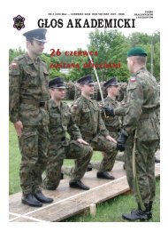
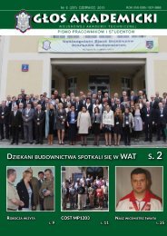
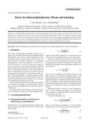
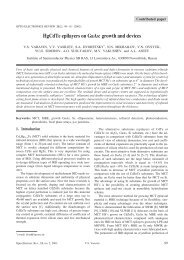
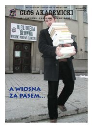
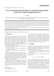
Improvement methods of reconstruction process in digital holography proach is applied less frequently. In the paper, a method decreasing the calculation time is proposed. 2. Method of noise reduction in the central part of holographic images Subtracting the average value of the intensity distribution from the holographic fringe image, the zero-order diffraction beam is removed. Afterwards, using Fourier transformation of the remaining intensity distribution the spectrum is received. It is presented in Fig. 1(a) in a pictorial manner, and in Fig. 1(b) for a laboratory realised hologram. Black central part in Fig. 1(b) results from the above mentioned subtractive pre-processing. However, three components real image, conjugate image, and a residuum from zero-order diffraction beam are present. The boundaries between the constitutive areas are never precisely well defined. Therefore it is difficult to elaborate an automatic program to separate the area of the demanded real image. We propose to make use of a symmetry property of the auto-correlation component with respect to the spectrum centre. Let h(x,y) be the intensity distribution at the hologram plane after subtracting its average value. Fourier transform u(m,n) of the intensity h(x,y) described by the following equation -1 u( m, n) = FFT [ h( x, y)] , (1) is a base to improve the holographic image quality. In general, the quantities m, n are the coordinates in the Fourier domain of the hologram intensity distribution, moreover, they have not be treated as physical parameters. It is worth emphasizing that in the case of Fourier hologram with an object situated at infinity these quantities take the role of angular coordinates. For the every spectrum column m, the centre of the intensity distribution and its shift with respect to the spectrum centre are determined by the following relation nG = å umnn ( , ) N åumn ( , ) , (2) N where N is the number of the samples in the every column. The distribution of the gravity centre vs. the column number, calculated for an exemplary object, is presented in Fig. 2. Choosing a level value of |n G –N 0 | denoting by d in Fig. 2 where N 0 =N 0 /2, the columns with the gravity centres below the chosen level are removed, what is described in mathematical form by the following equation ( G 0 ) " m Î á0, M Ù n - N < d Þ u( mn , ) = 0, (3) In consequence, majority of the spectrum related to the auto-correlation component is removed and the procedure result is presented in Fig. 3(a). The result received for laboratory hologram is shown in Fig. 3(b). Some non-zero columns, visible in the central part of Fig. 3(b) have no significant influence on the image quality due to the low spatial frequency filtration. In the next step, the conjugate image area is removed putting zero for all columns located at the conjugate image side, what is presented in Figs. 4(a) and 4(b). From the observer point of view it is more convenient to displace the spectrum gravity centre denoted by n c and m c , where mC åå åå umnm ( , ) umnm ( , ) N M N M = nC = ååumn ( , ) , ååumn ( , ) , (4) N M N M Fig. 1. Spatial spectrum of a typical hologram. Pictorial (a) and real (b) cases. 204 Opto-Electron. Rev., 11, no. 3, 2003 © 2003 COSiW SEP, Warsaw
Contributed paper Fig. 2. Gravity centre distribution for a chosen object. Fig. 3. Spatial spectrum after zero-order beam filtration. Pictorial (a) and real (b) cases. Fig. 4. Spatial spectrum after filtrating the zero-order beam and the conjugate image area. Opto-Electron. Rev., 11, no. 3, 2003 S. Paœko 205
Page 1: Contributed paper OPTO-ELECTRONICS
Page 5 and 6: Contributed paper h and r represent
Page 7 and 8: Contributed paper Fig. 10. Reconstr

Improvement methods of reconstruction process in digital holography

Create successful ePaper yourself

Delete template?

Save as template?